Polyelectrolyte stars in planar confinement

Abstract

We employ monomer-resolved Molecular Dynamics simulations and theoretical considerations to analyze the conformations of multiarm polyelectrolyte stars close to planar, uncharged walls. We identify three mechanisms that contribute to the emergence of a repulsive star-wall force, namely: the confinement of the counterions that are trapped in the star interior, the increase in electrostatic energy due to confinement as well as a novel mechanism arising from the compression of the stiff polyelectrolyte rods approaching the wall. The latter is not present in the case of interaction between two polyelectrolyte stars and is a direct consequence of the impenetrable character of the planar wall.

I Introduction

Polyelectrolytes (PE’s) are polymer chains that carry ionizable groups along their backbones. Upon solution in aqueous solvents, these groups dissociate, leaving behind a charged chain and the corresponding counterions in the solution. Chemically anchoring $f$ such PE-chains on a colloidal particle of radius $R_{\rm d}$ gives rise to a spherical polyelectrolyte brush (SPB). In the limit in which the height $R$ of the brush greatly exceeds $R_{\rm d}$, one talks instead about polyelectrolyte stars. A great deal of theoreticalpincus:91 ; klein:macromolecules:02 ; klein:macromolecules:99 ; borisov:jp:97 ; borisov:epjb:98 ; linse:macrom:00 ; arben:prl:02 ; arben:jcp:02 ; denton:pre:03 ; wang:denton:pre:04 ; norm:jcp:04 ; arben:cps:04 ; roger:epje:02 ; borisov:macrom:02 ; zhulina:macrom:02 ; borisov:macrom:03 ; arben:jcp:06 and experimentalguenoun:prl:98 ; maarel:macrom1:00 ; maarel:macrom2:00 ; maarel:langmuir:00 ; abraham:langmuir:00 ; ballauff:macrom:00 ; guo:pre:01 ; nico:02 ; heinrich:epje:01 ; maarel:prl:05 effort has been devoted in the recent past with the goal of understanding the conformations and the interactions of SPB’s and PE-stars. The reasons are many-fold. The grafted PE-chains can provide an electrosteric barrier against flocculation of the colloidal particles on which the chains are grafted, rendering the systems very interesting from the point of view of colloidal stabilization. Moreover, they can act as control agents for gelation, lubrication and flow behavior. From the point of view of fundamental research, PE-stars are a novel system of colloidal particles that combine aspects from two different parts of colloid science: polymer theory and the theory of charged suspensions. Accordingly, the derivation of the effective interaction between PE-stars has led to their description as ultrasoft colloids and to theoretical predictions on their structural and phase behaviorarben:jcp:02 ; norm:jcp:04 that have received already partial experimental confirmation.ishizu:mm:05 Moreover, certain similarities in the structural and phase behavior of PE-stars and ionic microgels have been established, demonstrating the close relationship between the two systems.dieter:prl:04 ; dieter:jcp:05

By and large, the theoretical investigations involving PE-stars have been limited to the study of either single PE-stars or bulk solutions of the same. However, a new field of promising applications and intriguing physics is arising when PE-stars or SPB’s are mixed with hard colloids or brought in contact with planar walls. Indeed, PE-stars can be used to model cell adhesion and are also efficient drug-delivery and protein-encapsulation and immobilization agents.riess:pps:03 ; bhatia:cocis:01 ; kakizawa:addr:02 ; biesh:jpcb:05 On the other hand, hydrogels, which are physically similar to PE-stars, adsorbed on planar walls, form arrays of dynamically tunable, photoswitchable or bioresponsive microlenses.kim:jacs:04 ; serpe:am:04 ; kim:ac:05 ; kim:jacs:05 The encapsulation properties as well as the characteristics of the microlenses depend sensitively on the interactions between the PE-stars and the colloidal particles or the wall, respectively. Therefore, there exists a need to undertake a systematic effort in trying to understand these interactions physically and make quantitative predictions about the ways to influence them externally. In this paper, we take a first step in this direction by considering a PE-star in the neighborhood of a planar, uncharged and purely repulsive wall. We analyze the mechanisms that give rise to an effective star-wall repulsion and identify the counterion entropy and the chain compression against the planar wall as the major factors contributing to this force. Our findings are corroborated by comparisons with Molecular Dynamics simulation results for a wide range of parameters that structurally characterize the stars. This work provides the foundation for examining effects of wall curvature and charge.

Our paper is organized as follows: Sec. II is devoted to the description of the system we are investigating, the simulation model, and the simulation techniques used. Moreover, we specify the physical quantities of interest. Our theoretical approach is addressed in detail in Sec. III. In Sec. IV, we quantitatively compare and discuss the respective results. Finally, we conclude and present an outlook to possible future work in Sec. V.

II Simulation model

We start with a definition of the system under consideration including its relevant parameters and a description of the simulation model used. We study a dilute, salt-free solution of PE-stars confined between two hard walls parallel to the $x$-$y$-plane at positions $z=\pm\tau/2$, resulting in an overall wall-to-wall separation $\tau$. We assume a good solvent that is only implicitly taken into account via its relative dielectric permittivity $\epsilon\approx 80$, i.e., we are dealing with an aqueous solution. To avoid the appearance of image charges,torrie:jcp:76 ; messina:jcp:117 we assume the dielectric constants to be the same on both sides of the respective confining walls. It turns out, however, that this is not a severe assumption, because the effective charge of a PE-star is drastically reduced compared to its bare value, due to the strong absorption of neutralizing counterions.klein:macromolecules:99 ; arben:prl:02 ; arben:jcp:02 ; konieczny:jcp:121 Hence, the influence of image charges can be expected to be of minor importance.

The PE-stars themselves consist of $f$ PE-chains, all attached to a common colloidal core of radius $R_{\rm d}$, whose size equals the monomer size and is therefore much smaller than the typical center-to-end length of the chains for all parameter combinations. The introduction of such a core particle is necessary to place the arms in the vicinity of the center, where the monomer density can take very high values. The theoretical approach pertains to the limit of vanishingly small core size. In order to remove effects arising from the small (but finite) value of the core in the simulation model and to provide a comparison with theory, we will henceforth employ a consistent small shift of the simulation data by $R_{\rm d}$. This standard approach has been applied already, e.g., to the measurement of the interactions between neutral jusufi:macromolecules:32 and charged stars arben:prl:02 ; arben:jcp:02 , in order to isolate the direct core-core interaction effects from the scaling laws valid at small interstar separations.

The PE-chains are modeled as bead-spring chains of $N$ Lennard-Jones (LJ) particles. This approach was first used in investigations of neutral polymer chains and stars stevens:prl:71 ; grest:macromolecules:20 ; grest:macromolecules:27 and turned out to be reasonable. The method was also already successfully applied in the case of polymer-colloid mixturesjusufi:jpcm:13 or polyelectrolyte systems.arben:prl:02 ; arben:jcp:02 ; konieczny:jcp:121 To mimic the above mentioned good solvent conditions, a shifted and truncated LJ potential is introduced to depict the purely repulsive excluded volume interaction between the monomers:

$$V_{\rm LJ}(r)=\begin{cases}4\varepsilon_{\rm LJ}\left[\left(\frac{\sigma_{\rm LJ}}{r}\right)^{12}-\left(\frac{\sigma_{\rm LJ}}{r}\right)^{6}+\frac{1}{4}\right]&r\leq 2^{1/6}\sigma_{\rm LJ}\\ 0&r>2^{1/6}\sigma_{\rm LJ}.\end{cases}$$ (1)

Here, $r$ is the spatial distance of two interacting particles. The quantities $\sigma_{\rm LJ}$ and $\varepsilon_{\rm LJ}$ set the basic length and energy scales for the system, respectively. In what follows, we fix the system’s temperature to the value $T=1.2\varepsilon_{\rm LJ}/k_{\rm B}$, where $k_{\rm B}$ denotes Boltzmann’s constant. The PE-chain connectivity is modeled by employing a standard finite extension nonlinear elastic (FENE) potential:grest:macromolecules:20 ; grest:macromolecules:27

$$V_{\rm FENE}(r)=\begin{cases}-\frac{k_{\rm FENE}}{2}\left(\frac{R_{0}}{\sigma_{\rm LJ}}\right)^{2}\ln\left[1-\left(\frac{r}{R_{0}}\right)^{2}\right]&r\leq R_{0}\\ \infty&r>R_{0},\end{cases}$$ (2)

with a spring constant $k_{\rm FENE}=7.0\varepsilon_{\rm LJ}$. The divergence length $R_{0}$ limits the maximum relative displacement of two neighboring monomers and is set to $R_{0}=2.0\sigma_{\rm LJ}$ in the scope of this work. The described set of parameters determines the equilibrium bond length, in our case resulting in a value $l_{0}=0.97\sigma_{\rm LJ}$.

When modeling the interactions between the monomers and a star’s colloidal core, the finite radius $R_{\rm d}$ of the latter has to be taken into account. All monomers experience a repulsive interaction with the central particle, in analogy to Eq. (1) reading as

$$V^{\rm c}_{\rm LJ}=\begin{cases}\infty&r\leq R_{\rm d}\\ V_{\rm LJ}(r-R_{\rm d})&r>R_{\rm d}.\end{cases}$$ (3)

In addition, there is an attraction between the innermost monomers in the arms’ chain sequence and the core which is of FENE type and can be written as (cf. Eq. (2)):

$$V^{\rm c}_{\rm FENE}=\begin{cases}\infty&r\leq R_{\rm d}\\ V_{\rm FENE}(r-R_{\rm d})&r>R_{\rm d}.\end{cases}$$ (4)

The chains are charged in a periodic fashion by a fraction $\alpha$ in such a way that every $(1/\alpha)$-th monomer carries a monovalent charge. Consequently, there is a total number of $N_{c}=\alpha fN$ monomer ions per PE-star. To ensure electroneutrality of the system as a whole, we include the same amount of oppositely charged, monovalent counterions in our considerations. Since the latter are able to freely move, they have to be simulated explicitly. Furthermore, they are of particular importance because they are expected to crucially affect the physics of the system. One example is the aforementioned fact that they induce a reduction of the stars’ bare total charges.

Two charged beads with spatial distance $r_{ij}$ interact by a full Coulomb potential, i.e., the electrostatic interaction energy is

$$\beta V_{\rm Coul}(r_{ij})=\beta\frac{q_{i}q_{j}e^{2}}{\epsilon r_{ij}}\equiv\lambda_{\rm B}\frac{q_{i}q_{j}}{r_{ij}}.$$ (5)

Thereby, $q_{i},q_{j}=\pm 1$ are the valencies of monomer ions and counterions, respectively, $e$ denotes the absolute value of the unit charge, and $\beta=1/k_{\rm B}T$ is the inverse temperature. In the above equation, the so-called Bjerrum length

$$\lambda_{\rm B}=\frac{\beta e^{2}}{\epsilon}$$ (6)

was introduced. It is defined as the distance at which the electrostatic energy equals the thermal energy. Thus, it characterizes the interaction strength of the Coulomb coupling. In the case of water at room temperature, one obtains $\lambda_{\rm B}=7.1\,{\rm{\AA}}$. In our simulations, we fix the Bjerrum length to $\lambda=3.0\sigma_{\rm LJ}$, thus corresponding to an experimental particle diameter $\sigma=2.4\,{\rm{\AA}}$. This is a realistic value for typical polyelectrolytes.essafi:jphys2f:5

For the purpose of completing the set of interaction potentials needed to describe the system at hand, we have to define particle-wall interactions. For technical reasons (see below), we do not regard the walls as true hard walls, as common in Monte-Carlo (MC) simulation studies.messina:langmuir:19 ; messina:macromolecules:37 Following the course of our above modeling and based on Eq. (1), we assume them to be of truncated-and-shifted-LJ type instead, leading to the following monomer-wall interaction:

$$V^{\rm w}_{\rm LJ}(z)=V_{\rm LJ}\left(\frac{\tau}{2}-z\right)+V_{\rm LJ}\left(\frac{\tau}{2}+z\right),$$ (7)

whereas $z$ refers to the $z$-component of the position vector of the particular bead. Likewise, the potential function for a star’s core interacting with the confining walls is yielded by combining Eqs. (3) and (7):

$$V^{\rm wc}_{\rm LJ}(z)=V_{\rm LJ}\left(\frac{\tau}{2}-R_{\rm d}-z\right)+V_{\rm LJ}\left(\frac{\tau}{2}-R_{\rm d}+z\right).$$ (8)

To finalize this section, we present a short summary of the simulation techniques used. We perform monomer-resolved Molecular Dynamics (MD) simulations in the canonical ensemble, employing a rectangular simulation box of total volume $V=M^{2}\tau$ that contains a single PE-star. We apply periodic boundary conditions in the $x$- and $y$-directions, while the box is confined with respect to the $z$-direction. Here, we always fix $M=\tau=120\sigma_{\rm LJ}$. This provides a sufficiently large simulation box to suppress any undesirable side-effects a priori and emulates a dilute solution of PE-stars (cf. above description of the physical problem under investigation). For the numerical integration of the equations of motion, we adopt a so-called Verlet algorithm in its velocity form.allen:book ; frenkel:book ; rapaport:book In order to stabilize the system’s temperature, we make use of a Langevin thermostatallen:book ; frenkel:book ; rapaport:book that introduces additional friction and random forces with appropriately balanced, temperature-dependent amplitudes. Due to the periodic boundary conditions and the long-range character of the Coulombic forces, a straight-forward calculation of the latter pursuant to Eq. (5) is not feasible. Therefore, we have to evaluate the forces using Lekner’s well-established summation methodlekner:physicaa:176 in its version for quasi two-dimensional geometries. Thereby, the convergence properties of the sums occurring during the computation are enhanced by a mathematically accurate rewriting, allowing a proper cut-off. For performance reasons, the forces have to be tabulated.

The typical time step is $\Delta t=0.002t_{0}$, with $t_{0}=(m\sigma_{\rm LJ}^{2}/\varepsilon_{\rm LJ})^{1/2}$ being the associated time unit and $m$ the monomer mass. In our case, the counterions are taken to have the same mass and size as the (charged) monomers.

In our simulations, we measure the effective core-wall forces as a function of the center-to-wall distance $D$. Furthermore, we examine various other static quantities and their $D$-dependence, namely the center-to-end distance $R$, the radius of gyration $R_{\rm g}$, the number of condensed counterions and the density profiles of all particle species involved. For this purpose, for every particular value of $D$ the system is equilibrated for about $5\times 10^{5}$ time steps. After this equilibration period, we perform production runs lasting between $1\times 10^{6}-2\times 10^{6}$ time steps. We carry out the above described measurements for a variety of arm numbers $f$ ($f=$10, 18, 30) and charging fractions $\alpha$ ($\alpha=$1/5, 1/4, 1/3) in order to make systematic predictions for the $f$- and $\alpha$-dependencies of all theoretical parameters. In all cases, we fix the degree of polymerization, i.e., the number $N$ of monomers per arm, to a value $N=50$.

III Theory of the effective PE-star–wall interaction

A PE-star in the neighborhood of a planar, impenetrable wall, undergoes conformational changes that modify its (free) energy in comparison to the value it has when the wall is absent or far away from the star. This separation-dependent difference between the free energies is precisely the effective interaction between the PE-star and the wall. There are three distinct mechanisms that give rise to an effective interaction in our case: the change in the electrostatic energy of the star, the change in the counterion entropy arising from the presence of the geometric confinement as well as contributions from compression of the stiff PE-chains against the flat wall. The former two are intricately related to each other, as the counterion distribution is dictated by the strong Coulomb interactions, hence they will be examined jointly, the latter is a distinct phenomenon arising in the presence of impenetrable walls.

III.1 The electrostatic and entropic contributions

To obtain theoretical predictions for the electrostatic-entropic contribution to the free energy for a PE-star close to a flat, hard wall, we employ a mean-field approach, inspired by and akin to that developed in Refs. klein:macromolecules:99, ; arben:prl:02, ; arben:jcp:02, , and konieczny:jcp:121, . Let $\rho_{\rm s}=N_{\rm s}/\Omega$ be the density of the solution of PE-stars, where $N_{\rm s}$ denotes the total number of PE-stars in the macroscopic volume $\Omega$. In general, a single PE-star of total charge $Q$ is envisioned as a spherical object of radius $R$, embedded in a spherical Wigner-Seitz cell of radius $R_{\rm W}$. Additionally, the latter contains $N_{\rm c}$ counterions, restricted to move in the Wigner-Seitz cell only and forming an oppositely charged background of total charge $-Q$. The cell’s radius is connected to the star density via $R_{\rm W}=(4\pi\rho_{\rm s}/3)^{1/3}$. In the case of center-to-wall separations smaller than $R_{\rm W}$ and/or $R$, we simply cut the counterion cloud and/or the star itself at the confining wall and treat them as chopped spheres instead of full spheres. Obviously, the compound system composed of a PE-star and its counterions is electroneutral as a whole. Since we are interested in the case of dilute PE-solutions only, we can limit ourselves to the consideration of a single PE-star. Clearly, for center-to-wall distances $D>R_{\rm W}$ there is no interaction between a PE-star and the wall within the framework of our theory. Accordingly, we will deal with the case $D\leq R_{\rm W}$ only. Fig. 1 sketches the physical situation and visualizes the decisive length scales of the problem.

A mechanism crucially influencing the physics of PE-systems is the so-called Manning condensation of counterions.manning:jcp:51-3a ; manning:jcp:51-3b ; manning:jcp:51-8 ; odijk:jpolymsci:16 ; winkler:prl:81 ; nyquist:macromolecules:32 ; jiang:jcp:110 ; deserno:macromolecules:33 A parameter indicating whether or not such a condensation effect will occur is the dimensionless fraction $\xi=\lambda_{\rm B}N\alpha/R$. If it exceeds unity, counterions will condense on the arms of the stars.manning:jcp:51-3a ; manning:jcp:51-3b ; manning:jcp:51-8 In our case, this condition is true for all parameter combinations examined (see below). Hence, the condensation effect has to be taken into account in our theoretical modeling. For that reason, we partition the counterions in three different states, an ansatz already put forward in Refs. arben:prl:02, ; arben:jcp:02, , and kramarenko:mts:9, : $N_{1}$ of the $N_{\rm c}$ counterion are in the condensed state, i.e., they are confined in imaginary hollow tubes of outer radius $\lambda_{\rm B}$ and inner radius $\sigma_{\rm LJ}$ around the arms of the star. The total volume accessible for the counterions in this state is $\Omega_{1}=\pi(\lambda_{\rm B}^{2}-\sigma_{\rm LJ}^{2})Rf$. A number of $N_{2}$ counterions is considered to be trapped in the interior of the star. These ions are allowed to explore the overall volume $\Omega_{\rm in}=\Omega_{\rm cs}(D,R)$ of the (possibly chopped) star except the tubes introduced above, i.e., $\Omega_{2}=\Omega_{\rm cs}(D,R)-\Omega_{1}$. Thereby, the volume $\Omega_{\rm cs}$ of a chopped sphere can be derived by straightforward calculations. With $\Omega(R)=4\pi R^{3}/3$, one obtains:

$$\frac{\Omega_{\rm cs}(D,R)}{\Omega(R)}=\begin{cases}\frac{1}{2}+\frac{3}{4}\left(\frac{D}{R}\right)-\frac{1}{4}\left(\frac{D}{R}\right)^{3}&D\leq R\\ 1&D>R.\end{cases}$$ (9)

Note that the total volume of the star is big compared to the volume of the tubes surrounding the arms, $\Omega_{\rm cs}(D,R)\gg\Omega_{1}$. Thus, we will make use of the approximation $\Omega_{2}\approx\Omega_{\rm cs}(D,R)$ in all steps to come. The remaining $N_{3}=N_{\rm c}-N_{1}-N_{2}$ counterions are able to freely move within the outer shell of volume $\Omega_{\rm out}=\Omega_{3}=\Omega_{\rm cs}(D,R_{\rm W})-\Omega_{\rm cs}(D,R)$ surrounding the star, where $\Omega_{\rm cs}(D,R_{\rm W})$ is the total volume of the Wigner-Seitz cell. The subdivision of counterions in the three different states is also depicted in Fig. 1, showing a star with 5 arms that are assumed to be fully stretched for demonstration.

The electrostatic and entropic part $V_{\rm ee}(D)$ of the effective interaction $V_{\rm eff}(D)$ between the PE-star and the wall, kept at center-to-wall distance $D$, results after taking a canonical trace over all but the star center degree of freedom. With ${\cal F}_{\rm ee}(D;R,\{N_{i}\})$ being the variational Helmholtz free energy for a system where a single star faces the confining wall, and which contains just the electrostatic and entropic parts, it is defined as:likos:physrep:348

$$V_{\rm ee}(D)=\min_{R,\{N_{i}\}}{\cal F}_{\rm ee}(D;R,\{N_{i}\}).$$ (10)

In principle, the equilibrium values of $R$ and $\{N_{i}\}$ are determined by the above minimization. We will discuss this point in more detail shortly. Note that we neglected a second, $D$-independent term on the right-hand side of Eq. (10) representing the contribution to the free energy for an infinitely large center-to-wall separation. Since it makes up a constant energy shift only, it does not influence the effective forces between the star and the wall we are mainly interested in. The electrostatic-entropic force contributions are obtained by differentiating with respect to $D$:

$$F_{\rm ee}(D)=-\frac{\partial V_{\rm ee}(D)}{\partial D}$$ (11)

Now, we derive concrete expressions for the terms of which ${\cal F}_{\rm ee}(D;R,\{N_{i}\})$ is built up, whereby we want to include both the counterions’ entropic contributions and the electrostatic energy. To keep our theory as simple as possible, we will omit other thinkable contributions, like elastic energiesdegennes:book of the chains or Flory-type terms arising through self-avoidance.degennes:book ; doi:book . As we will see in Sec. IV, our theoretical results in combination with chain-compression terms to be deduced in what follows, are capable of producing very good agreement between the theory and the corresponding simulational data; these simplifications are therefore a posteriori justified. Consequently, the free energy ${\cal F}_{\rm ee}(D;R,\{N_{i}\})$ reads as:

$${\cal F}_{\rm ee}(D;R,\{N_{i}\})=U_{\rm es}+\sum_{i=1}^{3}S_{i}.$$ (12)

The electrostatic mean-field energy $U_{\rm es}$ is assumed to be given by a so-called Hartree-type expression. Let $\rho_{\rm m}({\bf r})$ and $\rho_{i}({\bf r})$ denote the number densities of the monomers and the three different counterion species, respectively, measured with respect to the star’s geometrical center. These density profiles then determine the overall local charge density $\varrho({\bf r})$ of our model system. Therewith, we have:

$$U_{\rm es}=\frac{1}{2\epsilon}\iint{\rm d}^{3}r\;{\rm d}^{3}r^{\prime}\;\frac{\varrho({\bf r})\varrho({\bf r^{\prime}})}{\left|{\bf r}-{\bf r^{\prime}}\right|}.$$ (13)

It is convenient to separate the total charge density $\varrho({\bf r})$ into two contributions: $\varrho_{\rm in}({\bf r})$ in the interior of the star, i.e., the volume $\Omega_{\rm in}$, and $\varrho_{\rm out}({\bf r})$ in the outer region, i.e., the volume $\Omega_{\rm out}$. Let $\Phi_{\rm in}({\bf r})$ and $\Phi_{\rm out}({\bf r})$ be the contribution to the electrostatic potential at an arbitrary point ${\bf r}$ in space caused by the respective charge density. Using this definitions, we can rewrite Eq. (13) and get

$$U_{\rm es}= \frac{1}{2}\left\{\int_{\Omega_{\rm in}}{\rm d}^{3}r\;\left[\Phi_{\rm in}({\bf r})+\Phi_{\rm out}({\bf r})\right]\varrho_{\rm in}({\bf r})\right.$$

$$+\left.\int_{\Omega_{\rm out}}{\rm d}^{3}r\;\left[\Phi_{\rm in}({\bf r})+\Phi_{\rm out}({\bf r})\right]\varrho_{\rm out}({\bf r})\right\}.$$ (14)

On purely dimensional grounds, we expect a result having the general form

$$\beta U_{\rm es}= \frac{N_{3}\lambda_{\rm B}}{R}\cdot h\left(\frac{R_{\rm W}}{R},\frac{D}{R}\right)$$

$$= \frac{N_{3}\lambda_{\rm B}}{R}\left[h_{\rm in-in}\left(\frac{D}{R}\right)+2h_{\rm in-out}\left(\frac{R_{\rm W}}{R},\frac{D}{R}\right)\right.$$

$$+\left.h_{\rm out-out}\left(\frac{R_{\rm W}}{R},\frac{D}{R}\right)\right],$$ (15)

where we introduced dimensionless functions $h_{\alpha-\beta}$ arising from the integrations of the products $\Phi_{\alpha}({\bf r})\varrho_{\beta}({\bf r})$ in Eq. (III.1). Here, one should remember that $N_{3}$ is the number of uncompensated charges of the star and characterizes its effective valency. The specific shape of the $h$-functions depends on the underlying charge distributions $\varrho_{\rm in}({\bf r})$ and $\varrho_{\rm out}({\bf r})$ alone.

The terms $S_{i}$ represent the ideal entropic free energy contributions of the different counterion species. They take the form

$$\beta S_{i}= \int_{\Omega_{i}}{\rm d}^{3}r\;\rho_{i}({\bf r})\left[\log\left(\rho_{i}({\bf r})\sigma_{\rm LJ}^{3}\right)-1\right]$$

$$+3N_{i}\log\left(\frac{\Lambda}{\sigma_{\rm LJ}}\right),$$ (16)

where $\Lambda$ is the thermal de-Broglie wavelength. In writing the sum in Eq. (12), the respective last terms in Eq. (III.1) yield an trivial additive constant only, namely $3N_{\rm c}\log(\Lambda/\sigma_{\rm LJ})$, which will be left out in what follows.

Now, we have to quantitatively address the electrostatic and entropic terms pursuant to Eqs. (13) to (III.1) and (III.1). For that purpose, we first of all need to specify the above introduced number densities, $\rho_{\rm m}({\bf r})$ and $\rho_{i}({\bf r})$. Here, we model the arms of the PE-star to be fully stretched, or to put it in other words, the monomer density profile inside the star to fall of asklein:macromolecules:99 ; borisov:jp:97 ; borisov:epjb:98 ; arben:prl:02 $\rho_{\rm m}({\bf r})=\rho_{\rm m}(r)\sim r^{-2}$. This is a good approximation, as measurements yield a scaling behavior with an only somewhat smaller exponent $\cong-1.8$, indicating an almost complete stretching of the chains.arben:prl:02 ; arben:jcp:02 ; nyquist:macromolecules:32 ; brilliantov:prl:81 ; harnau:jcp:112 ; kantor:prl:83 Since the monomer ions are placed on the backbone of the chains in a periodical manner (cf. Sec. II), their density within the interior of the star must obviously show an identical $r$-dependence. Moreover, the profile for the trapped counterions exhibits the same scaling, due to the system’s tendency to achieve local electroneutrality.csajka:macromolecules:33 Therefore, it seems to be a good choice to use an ansatz $\rho_{2}(r)=A/r^{2}$ for the trapped counterions and $\varrho_{\rm in}(r)=B/r^{2}$ for the overall charge density in the inner region. Clearly, these distributions have to be normalized with respect to the total number of trapped counterions $N_{2}$ and the effective charge of the star $Q^{*}/e=(N_{\rm c}-N_{1}-N_{2})=N_{3}$ by integrating over the related volumes, $\Omega_{2}$ and $\Omega_{\rm in}$. In doing so, we obtain $A=N_{2}/(2\pi RC)$ and $B=Q^{*}/(2\pi RC)$, with

$$C=1+\frac{D}{R}\left[1-\log\left(\frac{D}{R}\right)\right].$$ (17)

We presume the condensed counterions to be uniformly distributed within the tubes surrounding the PE-chains, i.e., we use $\rho_{1}=N_{1}/\Omega_{1}$. This approach is supported by simulation results on single PE-chainswinkler:prl:80 and was successfully put forward in previous studies of PE-star systems.arben:prl:02 ; arben:jcp:02 In a similar fashion, we assume an also uniform distribution of the free counterions within the outer shell $R<r<R_{\rm W}$, i.e., $\rho_{3}=N_{3}/\Omega_{3}$, implying an associated charge density $\varrho_{\rm out}=-Q^{*}/\Omega_{3}$.

On this basis, we are able to explicitly calculate the variational free energy in virtue of Eqs. (12) to (III.1). As far as the entropic contributions are concerned, an analytical computation is feasible in a straightforward manner. For reasons of clarity, we leave out any intermediate steps and present our final results only:

$$\frac{\beta S_{1}}{N_{1}}= \log\left[\frac{N_{1}\sigma_{\rm LJ}^{3}}{\pi(\lambda_{\rm B}^{2}-\sigma_{\rm LJ}^{2})Rf}\right]-1,$$ (18)

$$\frac{\beta S_{2}}{N_{2}}= \log\left(\frac{N_{2}}{2\pi C}\right)+\frac{D}{RC}\log^{2}\left(\frac{D}{R}\right)$$

$$-3\log\left(\frac{R}{\sigma_{\rm LJ}}\right)+1,$$ (19)

$$\frac{\beta S_{3}}{N_{3}}= \log\left\{\frac{N_{3}}{\frac{2\pi}{3}\left[\left(\frac{R_{\rm W}}{R}\right)^{3}-1\right]+\frac{\pi D}{R}\left[\left(\frac{R_{\rm W}}{R}\right)^{2}+1\right]}\right\}$$

$$-3\log\left(\frac{R}{\sigma_{\rm LJ}}\right)-1.$$ (20)

Now, we want to investigate the electrostatic term $U_{\rm es}$ in more detail. To begin with, we have to derive expressions for the potential functions $\Phi_{\rm in}({\bf r})$ and $\Phi_{\rm out}({\bf r})$. This computations are rather technical and we will outline the course of action only. In general, the electrostatic potential $\Phi({\bf r})$ due to a charge density $\varrho({\bf r})$ in a dielectric medium is given by

$$\Phi({\bf r})=\frac{1}{\epsilon}\int{\rm d}^{3}r^{\prime}\;\frac{\varrho({\bf r}^{\prime})}{\left|{\bf r}^{\prime}-{\bf r}\right|}.$$ (21)

In order to calculate the integral above for a chopped sphere, yielding the function $\Phi_{\rm in}({\bf r})$, we decompose it in infinitesimally thin discs which are oriented perpendicular to the $z$-axis and cover the whole sphere. The radii of these discs obviously depend on their position with respect to the sphere’s center. Afterwards, each disc is object to further decomposition into concentric rings. Provided that the charge density is spherical symmetric, as is in the case under consideration, the charge carried by each ring can be easily calculated. The electrostatic potential of a charged ring is known from literature,jackson:book ; panofsky:book therefore the potential of a disc can be derived by integrating over all corresponding rings. An analytical determination of this integral is possible. The potential of the chopped sphere itself can then be obtained by another integration over all discs. The latter cannot be performed analytically, thus one has to resort to a simple, one-dimensional numerical integration. For a complete and explicit description of the procedure, we refer to Ref. arben:jcp:02, , Appendix A, where an almost identical derivation was put forward. So far, the potential $\Phi_{\rm out}({\bf r})$ caused by the hollow chopped sphere of volume $\Omega_{\rm out}$ containing the free counterions remains to be acquired. Thereto, we employ the superposition principle. The hollow region of uniform charge density $\varrho_{\rm out}({\bf r})$ can be apprehended as a superposition of two chopped spheres with radii $R$ and $R_{\rm W}$, and charge densities $-\varrho_{\rm out}({\bf r})$ and $\varrho_{\rm out}({\bf r})$, respectively. In doing so, the problem is reduced to the calculation of the electrostatic potential of a chopped sphere with uniform charge density, which can be computed following the method described above for the inner sphere of volume $\Omega_{\rm in}$ (see also Ref. arben:jcp:02, , Appendix B). Clearly, with knowledge of both $\Phi_{\rm in}({\bf r})$ and $\Phi_{\rm out}({\bf r})$, the dimensionless functions $h_{\alpha-\beta}$ and thus the electrostatic energy $U_{\rm es}$ can be obtained according to Eqs. (III.1) and (III.1) using numerical techniques.

In principle, the electrostatic-entropic interaction potential $V_{\rm ee}(D)$ is obtained by adding up the entropic and electrostatic contributions following Eq. (12) and minimizing the Helmholtz free energy ${\cal F}_{\rm ee}(D;R,\{N_{i}\})$ with respect to $R$ and $\{N_{i}\}$, cf. Eq. (10). However, the star radii are in good approximation unaffected by the center-to-wall separation $D$, as confirmed by our simulations. The physical reason lies in the already almost complete stretching of the chains due to their charging. In the simulation the radius $R$ of the star was measured according to

$$R^{2}=\frac{1}{f}\left<\sum_{\nu=1}^{f}\left({\bf r}_{\nu N}-{\bf r}_{0}\right)^{2}\right>,$$ (22)

where ${\bf r}_{\nu N}$ stands for the position vector of the last monomer of the $\nu$-th arm of the star and ${\bf r}_{0}$ the core position. Fig. 2 illustrates the weak $R$ vs. $D$-dependence for an exemplarily chosen parameter combination. Therefore, it is convenient not to determine $R$ through the variational calculation, but to use average values $\left<R\right>_{D}$ as obtained from MD simulations instead. The latter are comparable to the corresponding radii for isolated PE-stars according to Ref. arben:jcp:02, , see Table 1.

The amount of condensed counterions $N_{1}$ was measured by counting the number of such particles separated from the monomer ions by a distance smaller than $\lambda_{\rm B}$ and performing a statistical average. The total number of captured counterions, $N_{\rm in}=N_{1}+N_{2}$, was measured by counting all counterions within a sphere having the instantaneous, arm-averaged center-to-end distance and again taking a time average. Since the $\{N_{i}\}$ are related through the equation $N_{\rm c}=N_{1}+N_{2}+N_{3}$, only two independent variational parameters remain, say $N_{1}$ and $N_{2}$. In our simulations, we have found that the number of condensed counterions, $N_{1}$, is also approximately constant with respect to $D$, see Fig. 3. Hence, we will treat $N_{1}$ as a fit parameter, held constant for all $D$ and chosen in such a way to achieve optimal agreement with simulation results. Therefore, ${\cal F}_{\rm ee}(D;R,\{N_{i}\})$ is minimized with respect to the number of trapped counterions, $N_{2}$, only, reflecting the possibility of redistribution of counterions between inside/outside the stars as the distance to the wall is varied.

Fig. 4 shows a comparison of the entropic and the electrostatic contributions $S$ and $U_{\rm es}$ to the electrostatic-entropic effective potential, $V_{\rm ee}$. As one can see from the exemplary plot, the total entropic term $S$ is the major contribution to $V_{\rm ee}$ and therefore determines the functional form of the latter, while the electrostatic term is of minor importance. At first glance, this may seem to be counterintuitive in a PE-system, but electrostatics do in fact indirectly affect the interaction potential: Due to the presence of charges, the conformations and thus the radii of PE-stars are strongly changed compared to the neutral star case, leading to an increased range of the interaction. In the inset of Fig. 4 it can be seen that total entropy of the system at hand is mainly determined by the trapped counterions’ contribution $S_{2}$. As one can see, $S_{3}$ is only weakly influenced by the star-to-wall separation $D$, and $S_{1}$ is even completely independent of $D$, as was evident from Eq. (18). We have to emphasize, however, that even though $S_{1}$ contributes a constant value only and therefore does not influence the effective force $F_{\rm ee}(D)$ at all, the number of condensed counterions $N_{1}$ nevertheless plays an fundamental role in our problem. Since $N_{2}=N_{\rm in}-N_{1}$ set the overall scale for of the term $S_{2}$, $N_{1}$ becomes relevant in renormalizing the effective interaction. The treatment of $N_{1}$ and the net charge, consequently, as a fit parameter is a common approach for charged systems, known as charge renormalization.hansen:arpc:51 ; levin:physicaa:225 ; tamashiro:physicaa:258

III.2 The chain compression contribution

In anticipation of Sec. IV, we want to point out that significant deviations arise between the effective star-wall forces as obtained by our computer simulations and their theoretical counterparts $F_{\rm ee}$ calculated using the formalism presented in Sec. III.1 for intermediate center-to-surface distances $D/R\approx 0.6\ldots 1.3$. Now, we want to elucidate the physical mechanism leading to these deviations and derive simple expressions for additional contributions to both the total effective forces and potentials, $F_{\rm c}$ and $V_{\rm c}$. Therewith, we will conclude the development of our theoretical approach.

The need to introduce these supplementary contributions is due to so far unconsidered conformational changes enforced by the presence of the confining wall. During the construction of the mean-field part of our theory, we neglected such changes by assuming density profiles of monomers and counterions which are undisturbed compared to the case of isolated stars in full 3d geometries. The influence of the wall became manifest in a truncation of the spheres representing star and associated counterion cloud, only. But in reality, for $D$ in the order of the typical length of an arm of the star, the star will undergo strong configurational variations to avoid the wall since the monomers are not able to interpenetrate it. Thereby, due to the presence of neighboring arms, it can be energetically favorable for chains directing towards the wall to compress instead of bending away from the surface, although this compression leads to an extra cost in electrostatic energy. The latter obviously originates in a decrease of the ion-ion distances along the backbones of the chains. Figs. 5(a) and 5(b) depict the situation. Once a critical value of the chain length is reached, a further shortening of the chains under consideration becomes disadvantageous. Electrostatic repulsions and excluded volume interaction increase more and more strongly, the chains will preferably curve and start to relax in length, see Fig. 5(c). The occurrence of such compression-decompression processes is proved by our simulation runs.

In what follows, we will use a simplified picture and model the affected arms as rigid, uniformly charged rods of common length $L$ and diameter $\sigma_{\rm LJ}$ for both the compressed and the bent regime. In the former case, we assume the rods to have orientations perpendicular to the wall surface. In the latter case, we will account for the bending only via the re-lengthening of the rods and their change in orientation with respect to the $z$-axis. Fig. 5(c) visualizes this approximation, whereby the shaded straight chain represents the imaginary rod that replaces the bent arm within the framework of our modeling. The total charge of one such rod is just $qe\alpha N$, leading to an $L$-dependent linear charge density, $\eta$, given by $\eta=qe\alpha N/L$. We consider then the self-energy of one rod, as a function of its respective length $L$, to be made up of a purely repulsive contribution which is electrostatic in nature and arises due to like-charge repulsions, and a second harmonic term with an effective spring constant $k_{\rm eff}$ describing the binding of the chain monomers in a coarse-grained fashion. Thus, we have:nguyen:jcp:114

$$\beta U_{\rm rod}(L) =U_{\rm rep}(L)+U_{\rm attr}(L)$$

$$=\beta\frac{\eta^{2}}{\epsilon}L\ln\left(\frac{L}{\sigma_{\rm LJ}}\right)-\frac{k_{\rm eff}}{2}L^{2}$$

$$=\frac{Z^{2}\alpha^{2}N^{2}\lambda_{\rm B}}{L}\ln\left(\frac{L}{\sigma_{\rm LJ}}\right)-\frac{k_{\rm eff}}{2}L^{2}.$$ (23)

From Eq. (23), we then obtain the corresponding force $F_{\rm rod}(L)=-\partial U_{\rm rod}/\partial L$ that acts on the ends of the rod parallel to its direction (a negative/positive sign of $F_{\rm rod}(L)$ corresponds to a force that tends to compress/stretch the rod.) The competition of a repulsive and an attractive part results in a finite equilibrium length $L_{0}$ of the rod, i.e., $F_{\rm rod}$ vanishes for $L=L_{0}$. Clearly, $L_{0}$ is related to the above introduced spring constant $k_{\rm eff}$ by the following condition:

$$k_{\rm eff}=-\frac{1}{L_{0}}\left.\frac{\partial U_{\rm rep}}{\partial L}\right|_{L_{0}}.$$ (24)

Now, let $D_{\rm min}$ and $D_{\rm max}$ determine the range of center-to-surface distances for which the above described processes take place. Moreover, $D_{0}$ denotes the critical length for which the transition from the compressing to the bending regime is observed. According to our MD results, we will fix $D_{\rm max}/R=1.3$, $D_{0}/R=0.9$, and $D_{\rm min}/R=(2D_{0}-D_{\rm max})/R=0.5$. In addition, we require $L_{0}=D_{\rm max}$ in what follows. We know from our simulation runs that it is a reasonable first-order approximation to assume the length of the affected chains as a function of $D$ to be:

$$L(D)=\begin{cases}D_{\rm max}&D\in[0,D_{\rm min}[\\ 2D_{0}-D&D\in[D_{\rm min},D_{0}[\\ D&D\in[D_{0},D_{\rm max}]\\ D_{\rm max}&D\in[D_{\rm max},\infty[.\end{cases}$$ (25)

By using this empirical fact, we implicitly include effects due to chain bending and entropic repulsions of neighboring chains, even if we did not consider corresponding energy contributions explicitly in Eq. (23). Therewith, a promising estimate for the chain compression contribution to the total effective force is:

$$F_{\rm c}(D)=\begin{cases}f_{\rm eff}\frac{D}{L(D)}F_{\rm rod}(L(D))&D\in[D_{\rm min},D_{\rm max}]\\ 0&{\rm otherwise}.\end{cases}$$ (26)

Here, $f_{\rm eff}$ is the total number of affected chains. Assuming that the chains are regularly attached to the colloidal core, we expect a linear relation between $f_{\rm eff}$ and $f$, namely $f_{\rm eff}=f/f_{0}$. Simulation data indicate $f_{0}=4$ to be a good choice for all parameter combinations under investigation. Note that the pre-factor $D/L(D)=\cos\gamma$ results from geometrical considerations, as can be seen from Fig. 5(c).

Based on Eq. (26), we obtain the corresponding energy term $V_{\rm c}$ by a simple integration:

$$V_{\rm c}(D)=\int_{\infty}^{D}F_{\rm c}(D^{\prime})\;{\rm d}D^{\prime}.$$ (27)

Finally, the total effective forces and interaction potentials are obtained as the sum of the electrostatic-entropic and compression terms: $F_{\rm eff}=F_{\rm ee}+F_{\rm c}$ and $V_{\rm eff}=V_{\rm ee}+V_{\rm c}$, respectively. Fig. 6 shows a concluding comparison of the full effective potential $V_{\rm eff}(D)$ and the same without the inclusion of the compression term $V_{\rm c}(D)$. According to the plot, the theoretically predicted total potential is purely repulsive and ultra-soft. As we will see in Sec. IV, the total effective forces show a striking step-like shape for intermediate distances. This is in contrast to the well-known case of star-star interactions.arben:prl:02 ; arben:jcp:02

IV Comparison and discussion

In this section we test our theoretical model against corresponding simulation results to confirm its validity. Using standard MD techniques, a straightforward measurement of (effective) interaction potentials is not possible. Thereto, one would have to apply more sophisticated methods.watzlawek:book But since the mean force acting on the center of a PE-star can be easily received from computer experiments,jusufi:macromolecules:32 ; likos:physrep:348 we will focus on a comparison of such effective forces and corresponding theoretical predictions. To be more precise: when choosing the colloidal center of a star at a fixed position ${\bf r}_{\rm core}$ as effective coordinate in our simulations, the effective force can be measured as the time average over all instantaneous forces ${\bf f}_{\rm core}$ acting on the core (cf. also the simulation model in  Sec. II) by means of the expression:

$${\bf F}({\bf r}_{\rm core})=-\nabla_{{\bf r}_{\rm core}}V_{\rm eff}({\bf r}_{\rm core})=\left<{\bf f}_{\rm core}\right>.$$ (28)

In all considerations to come, we will deal with absolute values of the forces only. It is obvious from the chosen geometry that the effective forces are in average directed perpendicular to the confining wall, i.e., parallel to the $z$-axis. Thus, the mean values of the $x$- and $y$-components vanish, leading to the relation $F_{\rm eff}=\left|{\bf F}_{\rm eff}\right|=F_{{\rm eff},z}$. For symmetry reasons, the effective forces and potentials depend on the $z$-component of ${\bf r}_{\rm core}$ alone, whereas $r_{{\rm core},z}=D$. Consequently, the forces are connected to the potential by the following simple equation:

$$F_{\rm eff}({\bf r}_{\rm core})=F_{\rm eff}(D)=-\frac{\partial V_{\rm eff}}{\partial D}.$$ (29)

Therewith, predictions for the effective forces can be computed starting from theoretical results for the corresponding potential (see Sec. III, Fig. 6). This allows the desired comparison to MD data.

Fig. 7 shows typical simulation snapshots for two different values of the center-to-surface separation $D$, illustrating the conformational changes a star undergoes due to the presence of the confining wall. In part (b) of the figure, one may particularly note the PE-chains directed perpendicular to the wall. These arms are object to the compression-decompression mechanism described in detail in Sec. III.2 and sketched in Fig. 5. Moreover, the snapshots qualitatively visualize our quantitative finding that the majority of counterions is captured within the interior of a PE-star, cf. Fig. 3. We want to point out that, compared to the bulk case,arben:prl:02 ; arben:jcp:02 the counterion behavior in this regard is not significantly changed by introducing (hard) walls. In this context, we also refer to Table 1, where the number of condensed counterions $N_{1}$ as obtained from our MD runs is shown for different parameter combinations together with corresponding values for isolated PE-stars in unconfined geometries.

Fig. 8 is the core piece of this work and finally presents both our simulational and theoretical results for the effective star-wall forces. As can be seen from the plots, we find a very good agreement for all combinations of arm numbers and charging fractions. The theory lines exhibit a remarkable step-like shape for intermediate values of the center-to-surface distance $D$ arising due to the introduction of the chain compression term $F_{\rm c}$. The latter had to be added to the electrostatic-entropic forces $F_{\rm ee}$ to account for conformational changes induced by the spatial proximity of the star to the planar wall. In doing so, the functional form of the theoretically predicted forces accurately renders the results found by our computer experiments. When using the respective star’s radius as basic length scale for the plots, the position of the step is independent of the parameters considered. In this sense, the effect is universal and there is no influence by specific details of the system. Note that the distinct kink is an artifact resulting from the special construction of $F_{\rm c}$, it does not have any physical meaning. Again, it should be emphasized that the described behavior is in contrast to the well-known star-star case.arben:prl:02 ; arben:jcp:02 The difference between both systems mainly lies in the fact that a star is strictly forbidden to access the region of the wall, while it is allowed to interpenetrate another star-branched macromolecule to a certain degree. To put it in other words: a wall is impenetrable, while a second star is a diffuse, soft object. Here, we also want to emphasize that the step is no hysterisis/metastability effect, as in our MD simulations the center-to-surface separation $D$ is varied by pulling the stars away from the wall instead of pushing them towards it. This procedure prevents any coincidental trapping of individual PE-chains.

The particular values of the fit parameter $N_{1}$ used to calculate the theoretical curves in Fig. 8 are given in the corresponding legend boxes. Obviously, $N_{1}$ significantly grows with both the charging fraction $\alpha$ and the arm number $f$, as is physically reasonable. Table 1 compares the fit values used to their counterparts obtained by our simulations. Thereby, one recognizes systematic deviations, i.e., the fit values are always slightly off from the numbers computed using the MD method. Both quantities are of the order of 50-60% of the total counterion number, for all functionalities $f$ and charging fractions $\alpha$. The discrepancies emerge due to the different meanings of the quantities star radius $R$ and number of condensed counterions $N_{1}$. Within the scope of the simplified theoretical model, a PE-star is a spherical object of well-defined radius, while we observe permanent conformational fluctuations of the simulated stars. Thus, the MD radius does not identify a sharp boundary, but determines a typical length scale only. In this sense, the star can be viewed as a fluffy object. Most of the time, there are monomers, monomer ions and condensed counterions located at positions outside the imaginary sphere of radius $R$, and such counterions are not counted when measuring $N_{1}$, thus the theory value typically exceeds the simulation one. With increasing arm number $f$ and charging fraction $\alpha$, there is less variation in length of different arms of a star, resulting in smaller deviations between the theoretically predicted $N_{1}$ and its MD equivalent. Table 1 confirms this trend.

A last remark pertains to the behavior for small center-to-surface distances $D$. Since our simulation model includes a colloidal core of finite radius $R_{\rm d}$, the forces obtained from MD runs diverge for vanishing wall separations due to the core-wall LJ repulsion which mimics the excluded volume interaction. In contrast, our theoretical model has no core, for this reason the predicted forces remain finite for the whole range of distances. According to this, our theoretical approach is in principle not capable of reproducing a divergence of the forces, even in case of close proximity to the confining wall.

V Conclusions and outlook

We have measured by means of Molecular Dynamics simulations and analyzed theoretically the effective forces emerging when multiarm polyelectrolyte stars approach neutral, impenetrable walls. The forces have the typical range of the star radius, since osmotic PE-stars reabsorb the vast majority of the counterions and are thereby almost electroneutral; longer-range forces that could arise due to the deformation of the diffuse counterion layer outside the corona radius are very weak, due to the small population of the free counterion species. The dominant mechanism that gives rise to the soft repulsion is the entropy of the absorbed counterions and the reduction of the space available to them due to the presence of the impenetrable wall. At the same time, a novel, additional mechanism is at work, which stems from the compression of a fraction of the star chains against the hard wall. For star-wall separations that are not too different from the equilibrium star radius, the chain compression gives rise to an additional repulsive contribution to the force. At close star-wall approaches, the compressed chains ‘slip away’ to the side, orient themselves parallel to or away from the wall and thus the compression process ceases and the additional contribution to the force vanishes.

The compression force could play a decisive role in influencing the cross-interaction between PE-stars and spherical, hard colloids of larger diameter. Indeed, for this case, the cross-interaction could be calculated by using the results of the present work as a starting point and performing a Derjaguin approximation. It will be interesting to see what effects the cross-interaction has in the structural and phase behavior of such PE-star–colloidal mixtures. This issue, along with the study of the effects of charged walls and wall-particle dispersion forces, are the subject of ongoing work.

TABLES

Table 1: Conformational properties as obtained from MD simulations and corresponding fit parameters used in our theoretical approach for different arm numbers and charging fractions. In addition, results from Ref. arben:jcp:02, are presented for comparison. The chain length is fixed to $N=50$. For our data, the Wigner-Seitz radius is $R_{\rm W}/\sigma_{\rm LJ}=74.44$. Note that there are in part insignificant discrepancies between the parameters used here and in Ref. arben:jcp:02, .

$f$	$\alpha$	$N_{\rm c}$	$(R/\sigma_{\rm LJ})$	$(N_{1})$	$(N_{1})$	$(R/\sigma_{\rm LJ})$	$(N_{1})$
10	1/5	100	24.0	32	53	-	-
10	1/4	120	24.8	44	68	25.3	46
10	1/3	170	27.5	76	107	27.4	72
18	1/5	180	24.6	78	80	-	-
18	1/4	216	25.4	104	111	26.6	107
18	1/3	306	28.0	163	183	28.3	159
30	1/5	300	25.1	161	113	-	-
30	1/4	360	25.9	208	170	27.2	213
30	1/3	510	28.4	315	294	28.6	309

FIGURE CAPTIONS

FIG. 1: Sketch visualizing the physical situation at hand, namely showing a PE-star of typical spatial extent $R$, and its counterion background of radius $R_{W}$. The three possible counterion states are illustrated: Condensed, trapped, and free. For further explanations, see main text.

FIG. 2: Star radii vs. the star-wall separation $D$ as obtained by MD simulations, referring to parameters $f=10$, $\alpha=1/3$. The mean value, averaged with respect to $D$, is shown as a horizontal line for comparison.

FIG. 3: Fractions of condensed counterions $N_{1}/N_{\rm c}$ and captured counterions $N_{\rm in}/N_{\rm c}=(N_{1}+N_{2})/N_{\rm c}$ for PE-stars with $f=10$ arms and various values of $\alpha$. As one can see from the plots, both quantities are in very good approximation $D$-independent and the majority of counterions is captured within the interior of the star.

FIG. 4: Comparison of the entropic and the electrostatic contributions $S$ and $U_{\rm es}$ to the electrostatic-entropic part of the effective potential, $V_{\rm ee}$, exemplarily shown for $f=10$, $\alpha=1/3$, and $N_{1}=107$. Obviously, the entropic contribution dominantly determines the $D$-dependence of $V_{\rm ee}$. In the inset, $S$ is decomposed into the different counterion species’ contributions $S_{i}$, illustrating that the term $S_{2}$ governs the functional form of the total entropy. Note that the different contributions in both the main plot and the inset were shifted by constant values to enhance the readability of the plot.

FIG. 5: Schematic illustrating the physical mechanism leading to the necessity to introduce the energy contribution $V_{\rm c}$. Hollow circles denote neutral monomers, gray balls are monomer ions. The bigger black ball is the colloidal core of the star. Counterions are omitted in the depiction for reasons of clarity. In part (c) of the figure, the dashed rod replacing the chain bent to the left is shown mirror-reflected to the right to avoid crowding. For a more detailed discussion of the compression effect, see main text.

FIG. 6: Comparison of the total and the electrostatic-entropic contributions to the effective potential, $V_{\rm eff}(D)$ and $V_{\rm ee}(D)$, for $f=10$, $\alpha=1/3$, and $N_{1}=107$. The inset shows the functional form of the compression term $V_{\rm c}(D)$. The main text provides an explanation for the need of the latter contribution and contains an explicit derivation.

FIG. 7: Simulation snapshots of a PE-star with functionality $f=18$ and charging fraction $\alpha=1/3$. The center-to-wall distances are $D/R=0.107$ (a) and $D/R=1.07$ (b). Bright gray balls are neutral monomers, while the dark spheres along the chains indicate monomer ions. The counterions are the small, dark gray spheres surrounding the star.

FIG. 8: Effective star-wall forces with the colloidal core of the respective stars taken as effective coordinate, obtained from both computer simulations and our theoretical approach. The fit parameters $N_{1}$ used are specified in the legend boxes. Here, we show results for stars with functionalities $f=10$ (first row), $f=18$ (second row), and $f=30$ (third row). In all cases, we are considering charging fractions $\alpha=1/5$ (first column), $\alpha=1/4$ (second column), and $\alpha=1/3$ (third column). In the rightmost picture of the first row, we additionally included a theoretic line calculated without taking the compression term $V_{\rm c}$ into account to illustrate the need of such a contribution. Since the theoretical model has, in contrast to the simulation model, no (hard) colloidal core, all simulation data have to be displaced by the core radius $R_{\rm d}$.

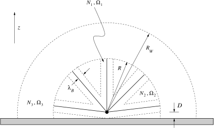
Figure 1: Konieczny, Likos

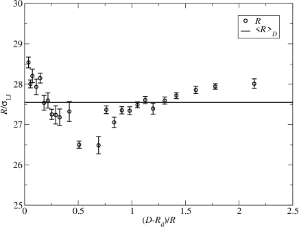
Figure 2: Konieczny, Likos

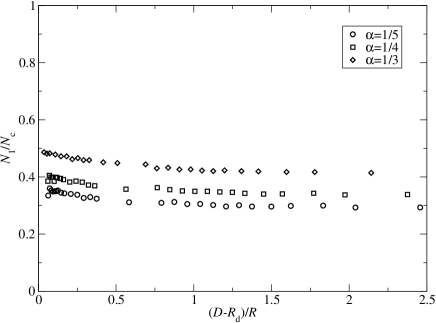
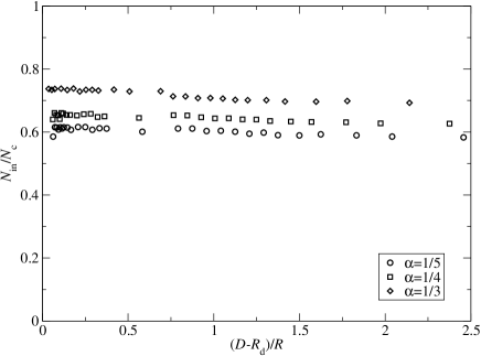
Figure 3: Konieczny, Likos

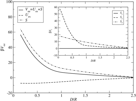
Figure 4: Konieczny, Likos

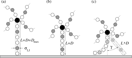
Figure 5: Konieczny, Likos

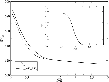
Figure 6: Konieczny, Likos

Figure 7: Konieczny, Likos

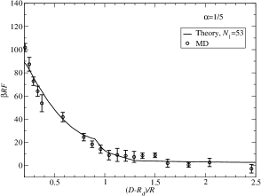
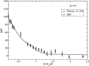
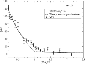
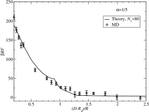
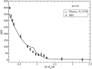
Figure 8: Konieczny, Likos