Ground-State and Domain-Wall Energies in the Spin-Glass Region
of the 2D $\pm J$ Random-Bond Ising Model

Abstract

The statistics of the ground-state and domain-wall energies for the two-dimensional random-bond Ising model on square lattices with independent, identically distributed bonds of probability $p$ of $J_{ij}=-1$ and $(1-p)$ of $J_{ij}=+1$ are studied. We are able to consider large samples of up to $320^{2}$ spins by using sophisticated matching algorithms. We study $L\times L$ systems, but we also consider $L\times M$ samples, for different aspect ratios $R=L/M$. We find that the scaling behavior of the ground-state energy and its sample-to-sample fluctuations inside the spin-glass region ($p_{c}\leq p\leq 1-p_{c}$) are characterized by simple scaling functions. In particular, the fluctuations exhibit a cusp-like singularity at $p_{c}$. Inside the spin-glass region the average domain-wall energy converges to a finite nonzero value as the sample size becomes infinite, holding $R$ fixed. Here, large finite-size effects are visible, which can be explained for all $p$ by a single exponent $\omega\approx 2/3$, provided higher-order corrections to scaling are included. Finally, we confirm the validity of aspect-ratio scaling for $R\to 0$: the distribution of the domain-wall energies converges to a Gaussian for $R\to 0$, although the domain walls of neighboring subsystems of size $L\times L$ are not independent.

I Introduction

The spin glass (SG) phaseEA75 ; reviewSG is not stable at finite temperature in two dimensions (2D). When the energies are not quantized, the behavior at $T=0$ can be understood in terms of a scaling theory,BM85 ; FH86 which is usually called the droplet model. This theory describes the scaling of the average domain-wall (DW) energy $E_{dw}$ with length scale in terms of the stiffness exponent $\theta$, i.e.

$$|E_{dw}|\sim L^{\theta}\,.$$ (1)

This exponent has a value of about $-0.28$ for 2D, almost independent of the detailed nature of the bond distribution AMMP03 and describes the scaling of different kinds of excitations like domain walls and droplets, at least if large enough system sizes are studied.droplet2003 The possibility that quantization of the energies might lead to the special behavior $\theta=0$ was first pointed out by Bray and Moore.BM86 It has become clear over the last few years that there actually is a fundamental difference in the behavior of the 2D Ising spin glass at zero temperature, between those cases where the energies are quantized and those where it is not.HY01 ; AMMP03 ; WHP03 Nevertheless, recent results JLMM06 ; Fis06 indicate that in the low-temperature critical scaling regime, the behavior for quantized and non-quantized models might be very similar.

The Hamiltonian of the Edwards-Anderson model for Ising spins is

$$H=-\sum_{\langle ij\rangle}J_{ij}{S}_{i}{S}_{j}\,,$$ (2)

where each spin ${S}_{i}$ is a dynamical variable which has two allowed states, $+1$ and $-1$. The $\langle ij\rangle$ indicates a sum over nearest neighbors on a simple square lattice of size $L\times M$. The standard model for quantized energies is the $\pm J$ model, where we choose each bond $J_{ij}$ to be an independent identically distributed (iid) quenched random variable, with the probability distribution

$$P(J_{ij})=p\delta(J_{ij}+1)~{}+~{}(1-p)\delta(J_{ij}-1)\,.$$ (3)

Thus we actually set $J=1$, as usual. The concentration of antiferromagnetic bonds is $p$, and $(1-p)$ is the concentration of ferromagnetic bonds. With the $P(J_{ij})$ of Eqn. (3), the EA Hamiltonian is equivalent to the $Z_{2}$ gauge glass model.ON93 Wang, Harrington and PreskillWHP03 have argued that the anomalous behavior of the $\pm J$ model is caused by topological long-range order, as a consequence of the gauge symmetry.

Along the $T=0$ axis this model exhibits a phase transition from a ferromagneticly ordered phase kirkpatrick1977 for small concentrations $p<p_{c}$ of the antiferromagnetic bonds to a SG critical line at large values $p>p_{c}$ (and $p<1-p_{c}$ due to the bipartite symmetry of the square lattice). Recently, this phase transition was characterized by high-precision ground-state calculations,WHP03 ; AH04 which have in particular yielded $p_{c}=0.103(1)$. The ferromagnetic phase persists at finite temperatures $T>0$ for $p<p_{c}(T)$, while the spin-glass correlations become long-range only at zero temperature.HY01 ; BM85 ; McM84b Interestingly, $p_{c}(T)>p_{c}(0)$,MerzChalker ; WHP03 ; AH04 i.e. the ferromagnetic phase is reentrant.

The first hint of the remarkable behavior of the $\pm J$ model in the SG regime was observed by Wang and Swendsen.WS88 They found that, although for periodic boundary conditions there is an energy gap of $4J$ between the ground states (GS) and the first excited states, the specific heat when $T/J\ll 1$ appeared to be proportional to $\exp(-J/2T)$.

This result was questioned by Saul and Kardar.SK93 ; SK94 The behavior of the specific heat was finally demonstrated in a convincing fashion by Lukic et al.LGMMR04 Saul and Kardar also found that the scaling of the DW entropy with size did not appear to agree with the prediction of the droplet model.FH88 This issue has recently been clarified,Fis06b and the DW entropy scaling anomaly has been associated with zero-energy domain walls.

In this work we explore the behavior of the $\pm J$ model inside the full SG phase $p_{c}\leq p\leq 0.5$ (the behavior $0.5\leq p\leq 1-p_{c}$ is equivalent due to the symmetry of the model). In particular we study the finite-size scaling behavior of the GS energy, of the fluctuations of the GS energy, and of the domain-wall energy. We also employ aspect-ratio (AR) scaling, FF69 ; PdN88 i.e. we study rectangular lattices of width $L$ and height $M$, the aspect ratio being $R=L/M$. Carter, Bray and MooreCBM02 have extended AR scaling to the Ising SG, and demonstrated that studying the scaling as a function of $R$ is an effective method for calculating the exponent $\theta$. Here, we look at the limit $R\to 0$ and show that AR indeed works for the $\pm J$ model as well, in contrast to previous attempts.HBCMY02 The entire probability distribution $P(E_{dw})$ has a simple Gaussian form for small $R$, although, as we will show, the underlying assumption of independent contributions to the DW energy is not strictly valid.

II Methods

We define domain walls for the SG as it was done in the seminal work of McMillan.McM84b We look at differences in the GS energy between two samples with the same set of bonds, and the same boundary conditions in one direction, but different boundary conditions in the other direction. In particular we use periodic (p) or antiperiodic (ap) boundary conditions along the x-axis and free boundary conditions along the y-axis. For an example of a DW created in such a way, cf. Fig. 11. For each set of bonds, the DW energy $E_{dw}$ is then defined to be the difference in the GS energies of the two different boundary conditions:

$$E_{dw}=E_{p}-E_{ap}\,.$$ (4)

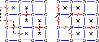
Figure 1: (color online) 2D Ising spin glass with all spins up (left, up spins not shown). Straight lines are ferromagnetic, jagged lines are anti-ferromagnetic bonds. The dashed lines connect frustrated plaquettes (crosses). The bonds crossed by the dashed lines are unsatisfied. In the right part the GS with three spins pointing down (all others up) is shown, corresponding to the minimum number of unsatisfied bonds.

We use a so-called matching algorithm to calculate the GS.PH-opt-phys2001 ; PH-opt-phys2004 Let us now sketch just the basic ideas of the matching algorithm. For the details, see Refs. bieche1980, ; SG-barahona82b, ; derigs1991, ; PH-opt-phys2001, . The algorithm allows us to find ground states for lattices which are planar graphs. This is the reason why we apply (anti-)periodic boundary conditions only in one direction, x, while the other direction, y, has free boundary conditions. In the left part of Fig. 1 a small 2D system with (for simplicity) free boundary conditions in both directions is shown. All spins are assumed to be “up”, hence all antiferromagnetic bonds are not satisfied. If one draws a dashed line perpendicular to each broken bond, one ends up with the situation shown in the figure: all dashed lines start or end at frustrated plaquettes and each frustrated plaquette is connected to exactly one other frustrated plaquette by a dashed line. Each pair of plaquettes is then said to be matched. In general, closed loops of broken bonds unrelated to frustrated plaquettes can also appear, but this is possible only for excited states. Now, one can consider the frustrated plaquettes as the vertices and all possible pairs of connections as the edges of a (dual) graph. The dashed lines are selected from the edges connecting the vertices and called a perfect matching, since all plaquettes are matched. One can assign weights to the edges in the dual graph, the weights are equal to the sum of the absolute values of the bonds crossed by the dashed lines. The weight $\Lambda$ of the matching is defined as the sum of the weights of the edges contained in the matching. As we have seen, $\Lambda$ counts the broken bonds, hence, the energy of the configuration is given by

$$E=-\sum_{\langle i,j\rangle}|J_{ij}|+2\Lambda\,,$$ (5)

with $|J_{ij}|=1$ from Eqn. (3). Note that this holds for any configuration of the spins, if one also includes closed loops in $\Lambda$, since a corresponding matching always exists.

Obtaining a GS means minimizing the total weight of the broken bonds (see right panel of Fig. 1). This automatically forbids closed loops of broken bonds, so one is looking for a minimum-weight perfect matching. This problem is solvable in polynomial time. The algorithms for minimum-weight perfect matchingsMATCH-cook ; MATCH-korte2000 are among the most complicated algorithms for polynomial problems. Fortunately the LEDA library offers a very efficient implementation,PRA-leda1999 which we have applied here.

With free boundary conditions in at least one direction, $E_{dw}$ is a multiple of 2 (since $J=1$). When periodic or antiperiodic boundary conditions are applied in both the x and y directions, however, $E_{dw}$ becomes a multiple of 4 if the number of $-1$ bonds is even. If the number of $-1$ bonds is odd, $E_{dw}$ takes on values $(4n+2)$ with these boundary conditions. When $M$ is odd, changing the boundary conditions in the x direction from periodic to antiperiodic changes the number of $-1$ bonds from odd to even, or vice versa.

The behavior of the DW energy for the $\pm J$ model with $R>1$ was discussed previously.HBCMY02 For the boundary conditions we are using, the average $\langle|E_{dw}|\rangle$ goes to zero exponentially as $R$ becomes much greater than one. Here $\langle...\rangle$ denotes an average over the ensemble of random bond distributions for an $L\times M$ lattice. We can understand this result by thinking of the system as consisting of blocks of size $M\times M$ pasted together along the x direction. The probability of having a zero-energy domain wall in each block is almost independent of the other blocks. The same thing happens when $M$ is even if the boundary conditions in the y direction are periodic or antiperiodic. However, if $M$ is odd and the boundary conditions in the y direction are periodic or antiperiodic, $\langle|E_{dw}|\rangle$ goes to 2 at large $R$, because then $E_{dw}=0$ is not allowed. Since a critical exponent should be independent of boundary conditions, this is a(nother) demonstration that $\theta=0$ for the $\pm J$ model in 2D.

As pointed out earlierHBCMY02 , these results for large $R$ do not agree with the scaling law prediction of Carter, Bray and Moore,CBM02 due to the special role of zero-energy domain walls. On the other hand, in the limit $R\to 0$ with our boundary conditions, the prediction of Carter, Bray and Moore is

$$\langle|E_{dw}|\rangle\sim L^{\theta}(M/L)^{(d-1)/2},~{}~{}M\gg L\,.$$ (6)

This limit has not been studied before for the $\pm J$ model. When $\theta=0$, $\langle|E_{dw}|\rangle$ should scale as $R^{-1/2}$ in 2D. For small $R$ we may think of the lattice as consisting of $L\times L$-sized subsystems stacked in the y direction, with $E_{dw}$ being the sum of the DW energies of the subsystems. Therefore, by the central limit theorem, we anticipate that the probability distribution of $E_{dw}$ should approach a Gaussian distribution in the limit of small $R$. In the spin-glass region of the phase diagram, the center of this limiting Gaussian will approach zero as $L$ increases. We will show that our numerical results for the small $R$ limit are indeed in good agreement with these expectations, even though the subsystems are not fully independent.

III Numerical Results

III.1 Ground-state energy

We begin the study of the $T=0$ behavior of the $\pm J$ random bond model by studying the GS energy for different concentrations $p$ of the antiferromagnetic bonds [$p=0.05$ (ferromagnetic phase), $p=0.11,0.12,0.13,0.14,0.15,0.17,0.2,0.25,0.3,0.35,0.4,0.45$ and $p=0.5$] and different system sizes $L=4,\ldots,320$ for square samples $N=L\times L$, i.e. aspect ratio $R=1$. All results are averages over many different realizations of the disorder. The minimum number of independent samples used varies with size, ranging between typically 100000 ($L=4$) to typically 10000 ($L=320$).

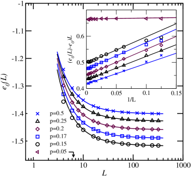
Figure 2: (color online) The symbols show the average ground state energy $e_{0}(L)$ for the square systems ($R=1$) as function of the system size $L$ for selected values of $p$. The lines give the results to the fits ($L\geq 16$) (see text). The data for $p=0.05$ look similar, but is outside the frame ($e_{0}=-1.8025$). The inset shows the same data, rescaled as $(e_{0}(L)-e_{0})\times L$ so that the expected behavior yields straight lines when plotted as function of $1/L$. The data for $p=0.05$ have been shifted downwards by 0.2 for better visibility.

In Fig. 2, the GS energy per spin $e_{0}(L)$ is shown as a function of the system size for selected values of $p$. This finite-size scaling behavior yields particular insight into the physics and seems to be related bouchaud2003 ; CHK04 to the stiffness exponent $\theta$. It has been argued CHK04 that for the case of open boundary conditions in exactly one direction and periodic boundary conditions in the other direction the GS energy per spin follows to lowest orders the form

$$e_{0}(L)=e_{0}+\frac{b}{L}+\frac{c}{L^{2}}+\frac{d}{L^{2-\theta}}\;.$$ (7)

Note that the arguments used in Ref. CHK04, should apply for the ferromagnetic phase $p\leq 0.103$ as well. Since we expect $\theta=0$ everywhere in the SG phase (see below) and $\theta=1$ for the ferromagnetic phase, we can restrict ourselves to the contributions $e_{0}$, $b/L$ and $c/L^{2}$. When fittinggnuplot the data to this $e_{0}(L)$, fits with very high quality result, as shown by lines in Fig. 2. This is confirmed when plotting the data and the fitting functions in the form $(e_{0}(L)-e_{0})L$ as a function of $1/L$. This should give, according to Eqn. (7), a linear behavior with slope $c$ and ordinate intersection $b$. We see that indeed the data follows the functional form well, although even higher order corrections seem to be present. They become significant at very small sizes, but we cannot quantify them within the statistical accuracy of the data. We only observe that this correction term seems to have an opposite sign for small ($p_{c}\leq p\leq 0.25$) compared to larger values of $p$. Furthermore, the behavior of the $c/L^{2}$ term is quite similar inside the SG phase for different values of $p$, while the behavior in the ferromagnetic phase $(p=0.05)$ is very different. The value of the ordinate intercept $b$ is monotonic in $p$, as expected.CHK04

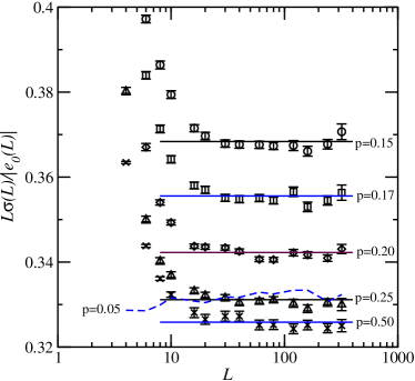
Figure 3: (color online) The symbols show the width $\sigma$ of the distributions of the GS energy $e_{0}$ for square systems ($R=1$) as function of system size $L$ for selected values of $p\geq p_{c}$. The data is rescaled with the average GS energy $e_{0}(L)$ and with the leading behavior $L$. Additionally, the dashed line displays the result for $p=0.05$. The full lines show fits to constants at larger system sizes.

Next, we consider the width $\sigma$ of the distribution of GS energies per spin. For short-range $d$-dimensional spin glasses, it has been proven wehr1990 that $\sigma\sim L^{-d/2}$, i.e. $\sigma\sim L^{-1}$ in this case. To remove finite-size effects caused by our special choice of boundary conditions, we normalize $\sigma$ by the finite-size GS energy. Thus, we plot $L\sigma/|e_{0}(L)|$ as a function of system size and expect a horizontal line at $c_{\sigma}(p)=\lim_{L\to\infty}L\sigma/e_{0}(L)$. As seen in Fig. 3, this is indeed the case. Only corrections for very small system-sizes become visible. We have also included the data for $p=0.05$, which behave in the same way. Hence, here the ferromagnetic phase and the SG phase cannot be distinguished just from the asymptotic behavior, in contrast to the behavior of the mean alone.

Figure 4: The symbols show the limiting value $c_{\sigma}(p)=\lim_{L\to\infty}L\sigma/e_{0}(L)$ for the width $\sigma$ of the distributions of the GS energy (as shown in Fig. 3) as a function of $p$. The solid line represents a fit according to Eqn. (8), see text.

On the other hand, as visible in Fig. 3, the value of $c_{\sigma}(p)$ increases when approaching the phase transition $p\to p_{c}$. For a more detailed analysis, we have plotted $c_{\sigma}(p)$ as function of $p$ inside the SG phase in Fig. 4, also for values of $p$ closer to $p_{c}$ than those shown in Fig. 3. One can see a strong increase when approaching the critical concentration. Fitting a power law (with $p_{c}=0.103$)

$$c_{\sigma}(p)=C_{c}+K(p-p_{c})^{\kappa}$$ (8)

in the range $p\in[0.1\ldots 0.17]$ yields values $C_{c}=0.422(3)$, $K=-0.38(4)$ and $\kappa=0.64(5)$, i.e. a cusp at the phase transition. Note that the value of the scaling exponent is very close to the exponent $\omega=2/3$, which describes the finite-size scaling of the DW energy $E_{dw}$; see below.

Nevertheless, the basic observation of the (almost) universal behavior inside the SG region, which we find when looking at the GS energy, becomes even more apparent, when studying the behavior of the DW energy, which we do in the next section.

III.2 Domain-wall energy

For all samples considered in the previous section, we have also calculated the DW energy as defined in Eqn. (4). In Fig. 5 the average value $\langle E_{dw}\rangle$ of the DW energy is shown as a function of system size for selected values of $p$. Close to the phase transition $p_{c}=0.103$, the systems exhibit a high degree of ferromagnetic order for small sizes, leading to relatively large values of the average DW energy. This explains why very large system sizes were needed in Ref. AH04, to determined the location $p_{c}=0.103$ of the phase transition precisely. For larger values $p\geq 0.2$, the ferromagnetic correlation length is small.

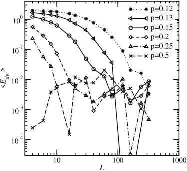
Figure 5: The average value of the DW energy as function of system size for selected values of $p$. Error bars are very small for values $\langle E_{dw}\rangle>0.1$ but relatively large where the DW energy is small. Thus, they are omitted for readability. Note the double-logarithmic axes. Lines are guides to the eye.

In Fig. 6 the average absolute value $\langle|E_{dw}|\rangle$ of the DW energy is shown as a function of system size for selected values of $p$. For very small values of $p$, close to the phase transition, this DW energy increases with system size for small system sizes. Hence, if only slow algorithm were available, the system would look like exhibiting an ordered phase (i.e. $\theta>0$). When going to larger system sizes, it becomes apparent that this is only a finite-size effect. For intermediate values of $p$, the DW energy decreases with growing system size, but no saturation of $\langle|E_{dw}|\rangle$ is visible on the accessible length scales, hence the data look similar to the results for Gaussian systems HY01 with $\theta<0$. When looking at the results for $p>0.25$, it becomes apparent that $\langle|E_{dw}|\rangle$ converges to a finite value. This is due to the quantized nature AMMP03 of the possible values for $E_{dw}$. Therefore, it is clear that also for intermediate values of $p$, the DW energy converges to a finite plateau-value as well, but for much larger system sizes. Hence, the model provides a striking example that finite-size corrections can persist up to huge length scales. Note that the convergence to a non-zero plateau value is compatible with the results from the previous section, where we have found that inside the SG phase the scaling function Eqn. (7) with $\theta=0$ describes the data well everywhere.

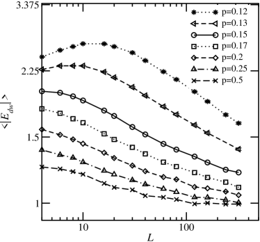
Figure 6: The average absolute value of the DW energy as a function of system size for selected values of $p$. Note the double-logarithmic axes. Lines are guides to the eye.

Due to the quantization of the possible DW energies, a value $\langle|E_{dw}|\rangle$ close to zero means that many system exhibit actual zero DW energy $E_{dw}=0$. We have also studied the finite-size dependence of the probability $P(E_{dw}=0)$ for a zero-energy DW as a function of the system size, as shown in Fig. 7. One observes that zero-energy domain walls are very common. Their probability of occurrence increases with the concentration $p$ of the antiferromagnetic bonds (until $p=0.5$ due to the symmetry of the model in $p,(1-p)$) and with the system size leading to a convergence to a limiting value for $L\to\infty$.

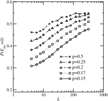
Figure 7: The probability $P(E_{dw}=0)$ for a zero-energy domain wall as function of system size for selected values of $p$. All error bars are at most of the symbol size. Lines are guides to the eye.

The simplest assumption for the convergence of $\langle|E_{dw}|\rangle$ and $P(E_{dw}=0)$, at given values of $p$, to their limiting values for $L\to\infty$ is a power law

$$F^{\star}(R,p,L)=A^{\star}(p,R)+B^{\star}(p,R)L^{-\omega^{\star}(p,R)}\,.$$ (9)

The exponent $\omega^{\star}$ describes the rate of convergence. It depends on the fraction $p$ of the antiferromagnetic bonds and on the aspect ratio $R$, as well as the constants $A^{\star}$ and $B^{\star}$. We have included the dependence on $R$ because below we also study values of $R<1$, but for the moment we stick to $R=1$.

Figure 8: The results of fitting Eqn. (9) to the data ($R=1$): exponent $\omega^{\star}$ (main plot) and limiting value $A^{\star}$ (inset).

When fitting Eqn. (9) to the DW energy data for $p\geq 0.15$, i.e. far enough away from $p_{c}$, and for sizes $L\geq 10$, we obtain results as shown in Fig. 8. For small concentrations $p$, the exponent $\omega^{\star}$ is less negative than for $p$ close to $0.5$, corresponding to needing larger sizes to reach the asymptotic value $A^{\star}$. On the other hand $A^{\star}$ itself seems to depend only weakly on $p$, confirming the notion that everywhere inside the SG region the DW energy reaches a non-zero plateau value. The dependence of $\omega^{\star}$ appears like a strong violation of universality inside the SG region. To investigate this assumption, whether it is a true non-universality or just a finite-size scaling effect, we have performed fits which also include corrections to scaling. We do this by fitting the data to a form

$$F(R,p,L)=A(R,p)+\sum_{m=1}^{m^{*}}B_{m}(R,p)L^{-m\omega}\,.$$ (10)

$F(R,p,L)$ represents any function of $P(E_{dw})$. Two examples that we chose to study were $\langle|E_{dw}|\rangle$ and the probability $P(E_{dw}=0)$.

The number of correction-to-scaling terms included, $m^{*}$, was chosen according to the amount of data to be fit. Here we have tried 2 and 3. Of course, the values of the coefficients $A$ and $B_{m}$ which are found by the fits depend somewhat on the choice of $m^{*}$. The computed statistical errors do not include any allowance for systematic errors due to the choice of the form of the scaling function. Fortunately, it turned out that the value of $A$ is relatively insensitive to the choice of $m^{*}$.

In general, whether we chose $m^{*}$ to be 2 or 3, the computed $B_{m}$ coefficients did not all have the same sign. This effect is caused by the behavior at small $L$. For this reason, there is no well defined prescription for deciding what the best choice of the exponent $\omega$ is. We have not included $\omega$ in the set of free fitting parameters. Since it is the purpose of this section to show that the behavior inside the full SG region is universal, we have selected a value for $\omega$, such that the data for all values of $p$ can be fit. Thus the strong finite-size effects close to $p_{c}$ can be explained also. We have chosen the value $\omega=2/3$, which is similar to the values used previously in other work on this model,HY01 ; WHP03 empirically. For a critical point with $T_{c}>0$, the general theory of finite-size scalingBar83 requires that $\omega=1/\nu$, where $\nu$ is the correlation length exponent. That result does not apply here, however, since $T_{c}=0$.

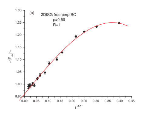
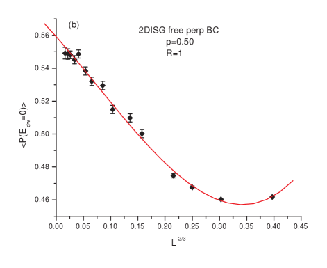
Figure 9: (color online) Finite-size scaling fits for $p=0.5$ and $R=1$: (a) $\langle|E_{dw}|\rangle$ vs. $L^{-2/3}$; (b) probability of $E_{dw}=0$ vs. $L^{-2/3}$. The error bars show one standard deviation.

As an example, our finite-size scaling fits (using $m^{*}=3$) to the data using Eqn. (10) for the case $p=0.5$ and $R=1$ are shown in Fig. 9, the data for all system sizes was included in the fits. In the figures, we show $F(R,L)$ as a function of $L^{-2/3}$. One observes a straight line for $L^{-2/3}\to 0$, showing that the choice of the exponent is compatible with the data. Note that the same $R=1$ data was originallyHY01 fit (only for the case $p=0.5$) by making different assumptions which are not consistent with Eqn. (10).

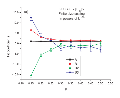
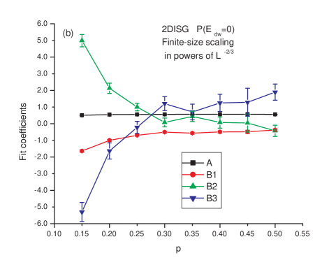
Figure 10: (color online) Fit coefficients (defined by Eqn. 10) for $R=1$: (a) $\langle|E_{dw}|\rangle$ vs. $p$; (b) $P(E_{dw}=0)$ vs. $p$.

Fig. 10(a) shows the fit coefficients for $\langle|E_{dw}|\rangle$, as defined by Eqn. (10), as a function of $p$ for $R=1$. The quality of fit was good everywhere, proving that the apparent non-universality visible in the dependence of the effective exponent $\omega^{\star}$ is due to the presence of corrections to scaling. We again see that the value of $A$, the estimate for $L\to\infty$, changes very little over this range of $p$; the values are for $p\geq 0.3$ very similar to the fit according to Eqn. (9), but they are larger in the present fit for small concentrations, $p<0.3$. We also note that there are substantial variations in the $B_{m}$ coefficients. In particular, $B_{3}$ alternates in sign for the smaller values of $p$. In Fig. 10(b) the results of fitting $P(E_{dw}=0)$, which shows the same type of behavior, are given. In this case the signs of $B_{2}$ and $B_{3}$ alternate.

III.3 Aspect-ratio scaling

Figure 11: Domain walls of subsystems are not independent: Comparison of a minimum-energy DW for a system of size $100\times 200$ (left) having $E_{dw}=2$ and of the same system cut into two systems of size $100\times 100$ (right), having $E_{dw}=0$. Note that in the left figure, the DW wraps around the system in the $x$-direction. Note also that the DWs are highly degenerate and the algorithm does not find DWs in a controlled way. A “jump” in the DW at the right is visible. This figure illustrates what a typical DW looks like. The important point here is the difference in the DW energies.

The main assumption when using AR scaling Eqn. (6) in the limit $R\to 0$ is that different subsystems of size $M\times M$ are independent of each other, which leads to a Gaussian distribution of the DW energies $E_{dw}$ in the limit $R\to 0$. Nevertheless, one can easily imagine that the DWs in different parts of the system are not truly independent of each other. This is demonstrated for a sample system in Fig. 11, where the DW energy of each subsystem (1)/(2) of size $100\times 100$ is $E_{dw}^{(1)/(2)}=0$, but the DW energy of the full system is $E_{dw}=2$. Also, in a previous study HBCMY02 , the validity of AR scaling could not be established for the $\pm J$ model. Here, we will show that AR scaling indeed works also for this case, i.e. the distribution of the DW energies becomes indeed Gaussian, despite the non-independencies of the domain walls inside the different subsystems. Because the shape of the $P(E_{dw})$ distribution is changing with $R$, we expect that the AR scaling will not be perfect in the range of our data. As we shall see, however, the deviations from the Gaussian fit become smaller than our statistical errors for $R\leq 1/4$. Thus we are able to verify that we are approaching the predicted scaling limit.

First, we concentrate on $p=1/2$ where the distribution $P(J_{ij})$ of Eqn. (3) is symmetric about zero. Thus in this case the distribution $P(E_{dw})$ is (ignoring statistical fluctuations) also symmetric around zero, for any values of $L$ and $M$. Therefore, we used $p=1/2$ to collect data for sets of random lattices with sequences of $L$ and $M$ having the aspect ratios $R$ = 1, 1/2, 1/4, 1/8, 1/16 and 1/32. For each value of $R$, we then used finite-size scaling to extrapolate to the large lattice limit.

Figure 12: The symbols display the distribution of DW energies for the case $L=M=40$ (i.e. $R=1$) and $p=0.5$, the lines shows the result of a fit to a Gaussian. Strong deviations from a Gaussian distribution are visible at $P(E_{dw}=0)$ (main plot) and in the “tail” of the distribution (inset).

We start by studying $L\times L$ samples ($R=1$), to establish that in this case the distribution of the DW energies is indeed not Gaussian. (Otherwise, it would not be surprising if it is also Gaussian for $R\ll 1$.) The distribution for $L=40$ is shown in Fig. 12. This distribution is obtained from an average over 39000 realizations. We have fitgnuplot a Gaussian to the data. (Note that the fitting procedure ignores the fact that the energies are quantized.) Strong deviations from Gaussian behavior are visible at $P(E_{dw}=0)$ (main plot) and in the “tail” of the distribution (inset). Correspondingly the quality of the fit, i.e. $\chi^{2}$ per degree of freedom, as given by our fitting programgnuplot in this case, is very high: $\chi^{2}/$ndf$=78$. Even larger deviations are expected in the tail. To observe these, more sophisticated techniques would be needed align ; 1dchain , which is beyond the scope of this work. The strong deviation from Gaussian behavior is not a finite-size effect, as may be seen from Fig. 13, where the circles display $\chi^{2}/$ndf as a function of $L$ for the $R=1$ case.

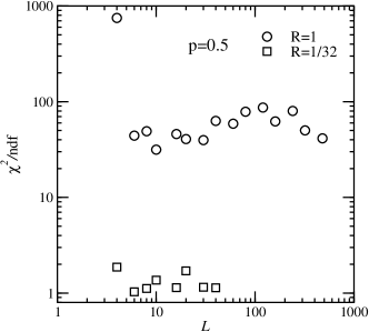
Figure 13: Quality of the Gaussian fit for the DW energy distribution measured by $\chi^{2}/$ndf as a function of the block size $L$ for $p=0.5$ (circles: $R=1$, squares: $R=1/32$).

The reader should also note that we find no evidence for any ”sawtooth” structure in the data. This is in marked contrast to the case of periodic or antiperiodic boundary conditions in the y direction, which causes alternating values of $E_{dw}$ to have zero probability. Therefore $P(E_{dw})$ does not become independent of the boundary conditions even in the limit of large lattices. This is an aspect of the topological long-range orderWHP03 which exists in this model when the boundary conditions are periodic along both x and y.

Figure 14: The symbols show the distribution of DW energies for the case $L=40,M=1280$ (i.e. $R=1/32$) and $p=0.5$, the lines shows the result of fitting to a Gaussian. Main plot: linear ordinate, inset: logarithmic ordinate scale. The data match the Gaussian very well.

In Fig. 14 we show the probability distribution $P(E_{dw})$ for a set of lattices with $p=1/2$, $R=1/32$ and $L=40$. In this case, there are 90,000 random samples in the data set. Again, the distribution was fit to a Gaussian gnuplot . This fit is quite good, as demonstrated by the fact that the value of $\chi^{2}/$ndf are is close to one. Note that the precise value of $\chi^{2}/$ndf depends on the number of points in the tail of the distribution that are included in the fit, which is somewhat arbitrary. The Gaussian behavior here is not a finite-size effect either. This can be seen from Fig. 13, where the square symbols display $\chi^{2}/$ndf as function of $L$ for the $R=1/32$ case.

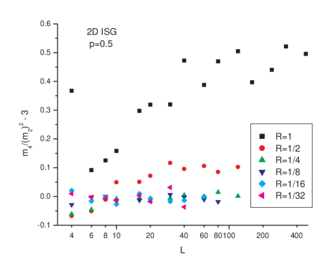
Figure 15: (color online) Kurtosis vs. $L$ ($p=0.5$.) The x axis is scaled logarithmically.

When $p=0.5$ the configuration averages of all the odd moments of $P(E_{dw})$ must vanish. Then the dominant contribution to non-Gaussian behavior will be the kurtosis, which simplifies to $m_{4}/(m_{2})^{2}-3$, where $m_{i}$ is the $i^{th}$ moment of $P(E_{dw})$, under these conditions. Fig. 15 shows the behavior of the kurtosis of the $P(E_{dw})$ distributions at $p=0.5$ as a function of $L$ and $R$. It shows that for $R\leq 1/4$ the kurtosis is negligible, except when $L<8$, quantifying the convergence towards a Gaussian distribution for small $R$.

This convergence can be also seen when fitting $\langle|E_{dw}|\rangle$ to Eqn. (10), now for aspect ratios $R<1$. In Table I we show the results of the finite-size scaling fits at $p=0.5$. According to Eqn. (6), the prediction of AR scaling theory is that the ratio $A(R)/A(2R)$ should approach $\sqrt{2}\approx 1.414$ for small $R$. Considering the statistical errors and the corrections to scaling, the agreement is quite satisfactory. Here we observe that for $R<1/4$ the scaling assumption is reasonably accurate.

Table 1: $\langle|E_{dw}|\rangle$ for $p=0.5$, extrapolated to $L=\infty$, as a function of the aspect ratio, $R$. The $m^{*}$ and $A$ are defined by Eqn. (10), and the $eA$ are statistical error estimates.

$R$	$m^{*}$	$A$	$eA$	$A(R)/A(2R)$
1.0	3	0.96025	0.00792
0.5	2	1.81967	0.00471	1.895
0.25	2	2.89085	0.00671	1.589
0.125	2	4.28859	0.01013	1.484
0.0625	2	6.21247	0.02387	1.449
0.03125	1	8.98954	0.03402	1.447

Table II shows the results of the finite-size scaling fits for the probability that $E_{dw}=0$ at $p=0.5$. Since, from the central limit theorem, for the sum $\Sigma$ of $K$ suitably iid integers, $P(\Sigma=0)\sim K^{-0.5}$, via $K\sim R^{-1}$ the prediction of AR scaling theory for this quantity is that the ratio $A(R)/A(2R)$ should approach $1/\sqrt{2}\approx 0.707$ for small $R$. Again, for $R<1/4$ the agreement is about as good as could be expected.

Table 2: Probability of $E_{dw}=0$ for $p=0.5$, extrapolated to $L=\infty$, as a function of the aspect ratio, $R$. The $m^{*}$ and $A$ are defined by Eqn. (10), and the $eA$ are statistical error estimates.

$R$	$m^{*}$	$A$	$eA$	$A(R)/A(2R)$
1.0	3	0.55921	0.00294
0.5	3	0.33215	0.00261	0.594
0.25	2	0.21619	0.00135	0.651
0.125	2	0.14736	0.00139	0.682
0.0625	2	0.10264	0.00144	0.697
0.03125	1	0.07053	0.00069	0.687

We have also studied the AR approach for $p=0.15$ and found similar results (not shown). For aspect ratios $R<1/4$ the assumptions of a Gaussian distribution of the DW energies is again valid. Hence, we believe that inside the entire SG region the behavior is consistent with the assumptions of the AR approach.

III.4 Discussion of AR scaling

At the end of Section II we argued that for small $R$ the system may be thought of as a set of $L\times L$ subsystems stacked in the y direction. This implies that the behavior of $E_{dw}$ in this limit should obey Eqn. (6) with $\theta=0$. As we have seen, our numerical results are indeed consistent with this argument. However, the hand-waving argument does not specify how the subsystems are to be connected to each other. Before actually seeing the numerical results, we were far from confident that this argument would correctly predict what was found.

There is another apparently reasonable argument, which leads one to expect that the results for small $R$ should not give this answer. As $R\to 0$, we know that the width of the $E_{dw}$ distribution will diverge. This means that for most of our sample lattices $|E_{dw}|\gg 1$ in this limit. One might have thought, therefore, that the fact that $E_{dw}$ is quantized would no longer matter. Thus one might have guessed that the system would behave in this limit as if $\theta\approx-0.28$, the value for an unquantized distribution.

Therefore, our results indicate that a Bohr correspondence principle, that in the limit of large quantum numbers the results should be indistinguishable from those of an unquantized system, does not apply. How can we understand this? In our opinion, what we learn from this is that $\theta=0$ is directly connected to the existence of topological long-range orderWHP03 at $T=0$.

One might try to argue that $R=1/32$ is not small enough, and that for even smaller $R$ one would indeed find a crossover to $\theta\approx-0.28$. Such a viewpoint is suggested by the recent work of Jörg et al.JLMM06 On the other hand a more detailed analysisFis06 of the low temperature behavior of the specific heat of the $\pm J$ model does not support this interpretation.

IV Summary

We have studied the statistics and finite-size scaling behavior of GS and DW energies for the 2D Ising random-bond spin glass with an mixture of $+1$ and $-1$ bonds, where $p$ is the concentration of antiferromagnetic bonds. By using sophisticated matching algorithms, we can calculate the GS energy and DW energies for quite large systems exactly, which allows us to study the scaling behavior very precisely. We find that the scaling behavior of the GS energy can be described everywhere inside the SG region by the same simple scaling function Eqn. (7), as predicted by Ref. CHK04, . Furthermore, when looking at the fluctuations of the GS energy, we find, after carefully taking into account finite-size corrections, that they follow the predicted simple $L^{-1}$-scaling with an amplitude which has a cusp singularity at the ferromagnetic-SG transition $p_{c}$. The singularity is described by an exponent which is close to $2/3$.

The behavior of the DW energy is characterized close to $p_{c}$, by huge finite-size effects. Nevertheless, the results are compatible with a convergence of $\langle|E_{dw}|\rangle$ to a finite plateau value everywhere inside the SG phase. This convergence can be described, again universally inside the SG phase, by a single exponent $\omega\approx 2/3$, just by taking into account higher-order corrections to scaling. Finally, we have studied $L\times M$ rectangular lattices with aspect ratio $R$ between 1/32 and 1. We have demonstrated by an example that one assumption underlying AR scaling, i.e. the assumed independence of the DW energies of different blocks, is not strictly valid. Nevertheless, we find that for large lattices the probability distribution of $E_{dw}$ in the SG region of the phase diagram approaches for $R\leq 1/4$ a Gaussian centered at $E_{dw}=0$. Hence, in the small $R$ limit the behavior obeys the AR scaling predictions of Carter, Bray and Moore.CBM02