Hydrodynamic mean field solutions of 1D exclusion processes with spatially varying hopping rates

Abstract

We analyze the open boundary partially asymmetric exclusion process with smoothly varying internal hopping rates in the infinite-size, mean field limit. The mean field equations for particle densities are written in terms of Ricatti equations with the steady-state current $J$ as a parameter. These equations are solved both analytically and numerically. Upon imposing the boundary conditions set by the injection and extraction rates, the currents $J$ are found self-consistently. We find a number of cases where analytic solutions can be found exactly or approximated. Results for $J$ from asymptotic analyses for slowly varying hopping rates agree extremely well with those from extensive Monte Carlo simulations, suggesting that mean field currents asymptotically approach the exact currents in the hydrodynamic limit, as the hopping rates vary slowly over the lattice. If the forward hopping rate is greater than or less than the backward hopping rate throughout the entire chain, the three standard steady-state phases are preserved. Our analysis reveals the sensitivity of the current to the relative phase between the forward and backward hopping rate functions.

1 Introduction

Asymmetric exclusion processes (ASEP) have been used as model nonequilibrium statistical mechanical systems to represent many physical processes such as traffic flow [1, 2, 3], ion transport across channels [4, 5], mRNA translation [6, 7, 8], and vesicle translocation along microtubules [9]. For uniform hopping rates, the steady-state currents, particle densities, and correlations of the one-dimensional totally (TASEP) and partially asymmetric exclusion process (PASEP) have been studied extensively using recursion methods, exact matrix product techniques, and mean field approximations [10, 11, 12, 13, 14]. The PASEP is described in Figure 1, and is comprised of one-dimensional lattice of sites, each of which can only be empty of singly occupied. The rules governing the dynamics of this system are as follows: a particle at site $n$ hops to site $n+1$ with probability $p_{n}\mbox{d}t$ in the time infinitesimal $\mbox{d}t$, only if site $n+1$ is empty. Similarly, it can hop backward to site $n-1$ (if site $n-1$ is empty) with probability $q_{n}\mbox{d}t$. At the left and right boundaries (sites $n=1$ and $n=N$, respectively) the injection probabilities are $\alpha\mbox{d}t$ and $\delta\mbox{d}t$, respectively, provided these sites are unoccupied. Extraction of particles from sites $n=1$ and $n=N$ occur at rates $\gamma$ and $\beta$, respectively. Particles do not hop if others are blocking their target sites. We will only consider the averaged steady-state configurations of this system.

Exact steady-state currents for the case of constant $p_{n}=p$ and $q_{n}=q$ have been found [13, 14]. In the case where $p\neq q$, the exact solution in the infinite lattice limit ($N\rightarrow\infty$) exhibits three phases described by maximal current, high particle density, and low particle density. Within each of these phases, the steady-state particle current is described by explicit analytical expressions [14]. Additional subphases corresponding to different density profiles arise within the high and low density current regimes [15, 16]. When the forward and backward hopping rates (out of and into each site) are equal, the chain is purely diffusive and is driven only by a difference between the injection/extraction rates at the boundaries. In this case, only a single, smooth (with respect to the injection/extraction rates) current phase exists.

In many systems modelled by the PASEP, the internal hopping rates are spatially varying. For example, variations in the hopping rates may arise in pores that have internal molecular structure, microtubules tracks (on which molecular motors move) that are comprised of periodic subunits, or from variations in mRNA or DNA sequence. Variations in the forward hopping rate for fixed lattice defects in a TASEP have been treated approximately in the limit of few, isolated defects [8, 17], and in the periodic case where the forward hopping rate takes on two values [18].

In this paper, we consider spatially varying internal forward and backward particle hopping rates in a PASEP. We find solutions for the current and density when the forward and backward hopping rates are given by functions $p_{n}$ and $q_{n}$ that vary slowly with the lattice position $n$. In the thermodynamic, mean field limit, the equation of motion for the mean occupancy at each site can be described in terms of a nonlinear continuum equation involving the coarse grained mean occupations $\sigma(x)$, and the continuum hopping rate functions $p(x)$ and $q(x)$. In the next section we derive the steady-state continuum equations by expanding the occupancy evolution equations in powers of $\varepsilon=1/N$, where $N\rightarrow\infty$ is the total number of lattice sites in the chain. We the consider four general classes of the hopping functions $p(x)$ and $q(x)$. In Section 3, we treat the “pure diffusion” limit where $p_{n}=q_{n+1}$, or, in the continuum limit, $p(x)=q(x+\varepsilon)$. In this limit, $q(x)\simeq p(x)-\varepsilon p^{\prime}(x)$, the mean-field equations become linear, and exact simple results are recovered. In Section 4, we consider the “shifted diffusion” limit, where the forward and backward hopping rates at each site are identical in the sense that $p_{n}=q_{n}$, or, $|p(x)-q(x)|\ll o(\varepsilon)$. We find exact implicit solutions for special forms of $p(x)$,. These results are markedly different from those found for pure diffusion, although the structure of $p(x)$ and $q(x)$ are nearly identical for the two cases. The case where $|p(x)-q(x)|>O(\varepsilon)$, and $p(x)-q(x)$ does not change sign is considered in Section 5. Asymptotic analysis indicates that the standard three phase structure found for constant $p,q$ [13, 14] is preserved qualitatively. In Section 6, we show that internal density boundary layers arise if $p(x)-q(x)$ crosses zero for $0<x<1$. This case eluded analytic treatment so only numerical and simulation results were obtained. In all cases, we compare our results with numerics and continuous time Monte-Carlo simulations. In the Summary and Conclusions, we discuss the limits in which one would expect mean-field approaches to yield exact steady-state currents.

2 Continuum Mean Field Limits

Figure 1: The $N+1$-site open boundary, partially asymmetric exclusion process. The continuum limit is a taken by setting each lattice site to size $\varepsilon=1/N$, thereby normalizing normalizing the total length.

Consider a one-dimensional lattice (Fig. 1) containing $N+1$ sites each of length $\varepsilon$. For the interior sites, the continuum limit of this lattice will be defined by a sampling of all relevant quantities (e.g., density) at the centers of each lattice site. Density profiles in the presence of sources and sinks exhibit rich shock behavior as studied by Parmeggiani et al. [19], and by Evans et al. [20]. Here, we will neglect adsorption/desorption at the interior sites; however, we allow the internal hopping rates to vary slowly along the chain.

The equation for the discrete occupation variable $\hat{\sigma}_{n}\in(0,1)$ in the chain interior is

$$\begin{array}[]{ll}\displaystyle{\mbox{d}\hat{\sigma}_{n}\over\mbox{d}t}&=(\hat{J}_{n-1}^{+}-\hat{J}_{n}^{+})+(\hat{J}_{n+1}^{-}-\hat{J}_{n}^{-}),\quad 1\leq n\leq N-1,\end{array}$$ (1)

where

$$\hat{J}_{n}^{+}=p_{n}\hat{\sigma}_{n}(1-\hat{\sigma}_{n+1})\quad\mbox{and}\quad\hat{J}_{n}^{-}=q_{n}\hat{\sigma}_{n}(1-\hat{\sigma}_{n-1})$$ (2)

are the currents from site $n$ to site $n+1$ and from site $n$ to site $n-1$, respectively.

The mean field assumption implies that the ensemble averaged occupancies are uncorrelated, $\langle\hat{\sigma}_{n}\hat{\sigma}_{m}\rangle\approx\sigma_{n}\sigma_{m}$, where $\sigma_{n}\equiv\langle\hat{\sigma}_{n}\rangle$. Upon taking an ensemble average of Eq. 1, and applying the mean field approximation, the evolution equation for the mean occupancy in the chain interior $(1\leq n\leq N-1)$ becomes

$$\begin{array}[]{ll}\displaystyle{\mbox{d}\sigma_{n}\over\mbox{d}t}&=(J_{n-1}^{+}-J_{n}^{+})+(J_{n+1}^{-}-J_{n}^{-})\\[13.0pt] &\displaystyle\approx\varepsilon{\partial\over\partial x}(J^{-}-J^{+})+{\varepsilon^{2}\over 2}{\partial^{2}\over\partial x^{2}}(J^{+}+J^{-}).\end{array}$$ (3)

where $J_{n}^{+}\equiv\langle\hat{J}_{n}^{+}\rangle=p_{n}\sigma_{n}(1-\sigma_{n+1})$ and $J_{n}^{-}\equiv\langle\hat{J}_{n}^{-}\rangle=q_{n}\sigma_{n}(1-\sigma_{n-1})$. Upon extrapolating the continuous function according to $\sigma(x=n\varepsilon)=\sigma_{n}$, and Taylor expanding Eq. 3 in powers of $\varepsilon$, we find the continuum mean field equation:

$$\hskip 42.67912pt{\mbox{d}\sigma(x)\over\mbox{d}t}=\varepsilon\left[(q-p)\sigma(1-\sigma)\right]^{\prime}+{\varepsilon^{2}\over 2}\left[\left[(p+q)\sigma\right]^{\prime}(1-\sigma)+(p+q)\sigma\sigma^{\prime}\right]^{\prime}.$$ (4)

Assuming the steady-state limit, and integrating the conservation Eq. 4, we obtain [21]

$$(p-q)\sigma(1-\sigma)-{\varepsilon\over 2}\left(\left[(p+q)\sigma\right]^{\prime}(1-\sigma)+(p+q)\sigma\sigma^{\prime}\right)=J,$$ (5)

where the integration constant $J$ is the steady-state current. Equation 5 can be rewritten in the Riccati form

$$\varepsilon\sigma^{\prime}(x)=-JP(x)+Q(x)\sigma(x)(1-\sigma(x)),$$ (6)

where

$$\begin{array}[]{l}\displaystyle P(x)={2\over(p+q)}\quad\mbox{and}\\[13.0pt] \displaystyle Q(x)=\left[{2(p-q)\over(p+q)}-\varepsilon{(p+q)^{\prime}\over(p+q)}\right].\end{array}$$ (7)

The boundary densities are found by measuring the steady-state current into and out of the first and last sites: $J=\alpha(1-\sigma_{0})-\gamma\sigma_{0}$ and $J=\beta\sigma_{N}-\delta(1-\sigma_{N})$, from which we find

$$\sigma_{0}={\alpha-J\over\alpha+\gamma}\quad\mbox{and}\quad\sigma_{N}={\delta+J\over\beta+\delta}.$$ (8)

Equations 6 and 8 form the basis of our steady-state analysis. Integrating Eq. 6 from $x=0$ to $x=1$, and imposing the boundary conditions (Eqs. 8), implicitly determines $J$. Once the steady-state current $J$ is fixed, the mean field density profiles are determined. For certain $p(x),q(x)$, one may be able to solve Eq. 6 analytically, and use this result along with the boundary conditions 8 to find $J$ in closed form.

3 Pure diffusion: $p(x)=q(x+\varepsilon),\,0<x<1$

Consider the special case $p_{n}=q_{n+1},\,\,1\leq n\leq N-1$ where the hopping rates between two sites are equal. In this case, there is no driving force on the particles and a net current arises only from differences in injection and extraction rates at the two ends. The quadratic terms in Eq. 1 cancel, the equation for $\sigma_{n}$ becomes linear, and the mean field approximation is exact. In the continuum approximation $p(x)=q(x+\varepsilon)$,

$$P(x)={1\over p(x)}\left[1+{\varepsilon\over 2}{p^{\prime}\over p}+{\varepsilon^{2}\over 4}\left({p^{\prime 2}\over p^{2}}-{p^{\prime\prime}\over p}\right)^{2}+O(\varepsilon^{3})\right]\,\,\mbox{and}\,\,Q(x)=O(\varepsilon^{3}),$$ (9)

and to lowest order in $\varepsilon$,

$$\sigma^{\prime}(x)\simeq-{J\over\varepsilon p(x)}.$$ (10)

Integration of Eq. 10 yields

$$\sigma(1)-\sigma(0)\approx-{J\over\varepsilon}\int_{0}^{1}{1\over p(x^{\prime})}\mbox{d}x^{\prime}\equiv-{J\over\varepsilon}\langle 1/p\rangle.$$ (11)

Upon applying Eqs. 8, (with $q_{1}=p_{0}$ and $q_{N}=p_{N-1}$), and solving for $J$,

$$J={(\alpha\beta-\gamma\delta)\over\langle 1/p\rangle(\alpha+\gamma)(\beta+\delta)+(\alpha+\beta+\gamma+\delta)}.$$ (12)

This same “homogenization” result, with the Riemann equivalent

$$\langle 1/p\rangle\equiv\sum_{n=0}^{N-1}p_{n}^{-1},$$ (13)

is also easily obtained by recursively solving the exact discrete equation $p_{n-1}(\sigma_{n}-\sigma_{n-1})=-J,\,(1\leq n\leq N)$. The corresponding density profile is obtained through

$$\sigma_{n}=\sigma_{0}+J\sum_{j=0}^{n-1}p_{j}^{-1}.$$ (14)

For constant $p_{n}=q_{n}=p$, Eq. 12 reduces to trivial result for the steady-state current of an $N+1$ site boundary-driven chain [4, 14]

$$J={p(\alpha\beta-\gamma\delta)\over N(\alpha+\gamma)(\beta+\delta)+p(\alpha+\beta+\gamma+\delta)}.$$ (15)

4 Shifted diffusion: $p(x)\simeq q(x),\,0<x<1$

If $p_{n}\simeq q_{n}$, such that $|p(x)-q(x)|\ll o(\varepsilon)$, particles at each site hop equally to the right or the left, with possibly different rates from site to site. This case corresponds to particles that cannot distinguish forward from backward motion but, as detailed balance is violated, is not equivalent to pure diffusion. We will see that this slight change in the hopping rate structure from the $p_{n}=q_{n+1}$ case results in a very different steady-state current.

To lowest order, when $p(x)\simeq q(x)$,

$$P(x)\simeq{1\over p(x)}\quad\mbox{and}\quad Q(x)\simeq-\varepsilon{p^{\prime}(x)\over p(x)}.$$ (16)

Since $Q(x)$ is of order $P(x)$, the $\sigma(1-\sigma)$ term in Eq. 6 cannot be neglected and, unlike the purely diffusive case, the problem is nonlinear. Therefore, we would not expect the mean field particle densities or currents to be necessarily exact.

In this case, there are various variable transforms that render the Riccati equation analytically tractible. The simplest case is where the Riccati equation is separable. This occurs when $(p+q)^{\prime}=$constant, which implies $p(x)=q(x)=ax+b$. Equation 6 can then be integrated from $x=0$ and $\sigma=\sigma(0)=\sigma_{0}$ to give

$$\int_{0}^{x}{\mbox{d}x^{\prime}\over ax^{\prime}+b}={1\over a}\int_{\sigma_{0}}^{\sigma(x)}{\mbox{d}\sigma\over(\sigma-\sigma_{+})(\sigma-\sigma_{-})},$$ (17)

where $\sigma_{\pm}=1/2\pm 1/2\sqrt{1+4J/(\varepsilon a)}$. Integrating (17), we find the density profile $\sigma(x)$ from

$$\left({ax+b\over b}\right)^{\sigma_{+}-\sigma_{-}}=\left({\sigma(x)-\sigma_{+}\over\sigma(x)-\sigma_{-}}\right)\left({\sigma_{0}-\sigma_{-}\over\sigma_{0}-\sigma_{+}}\right).$$ (18)

An implicit formula for $J$ (to order $\varepsilon$) is found by imposing the boundary condition at $x=1$ ($\sigma(1)=\sigma_{N}\approx\delta/(\beta+\delta)$):

$$\left({a+b\over b}\right)^{\sqrt{1+4J/(\varepsilon a)}}=\left({\delta-(\beta+\delta)\sigma_{+}\over\delta-(\beta+\delta)\sigma_{-}}\right)\left({\alpha-(\alpha+\gamma)\sigma_{-}\over\alpha-(\alpha+\gamma)\sigma_{+}}\right).$$ (19)

The solution to Eq. 19 is found numerically and plotted in Fig. 2 for representative parameters.

Next, consider another analytic solution found by using the definition

$$\sigma(x)={\varepsilon\over Q(x)}{y^{\prime}(x)\over y(x)}$$ (20)

which transforms Eq. 6 to

$$Q(x)y^{\prime\prime}(x)-\left[Q^{\prime}(x)+\varepsilon^{-1}Q^{2}(x)\right]y^{\prime}(x)+\varepsilon^{-2}JP(x)Q^{2}(x)y(x)=0.$$ (21)

Provided

$$Q^{\prime}(x)+\varepsilon^{-1}Q^{2}(x)=0,$$ (22)

and $Q(x)\neq 0$, we find

$$y^{\prime\prime}(x)+\varepsilon^{-2}JP(x)Q(x)y=0.$$ (23)

The condition Eq. 22 is solved by

$$Q(x)={\varepsilon\over x+b}\equiv{2(p-q)\over(p+q)}-{\varepsilon(p+q)^{\prime}\over(p+q)},$$ (24)

which constrains $q(x)$ to $p(x)$ through

$$q(x)={e^{-2x/\varepsilon}\over x+b}\left[\int^{x}(x^{\prime}+b)g(x^{\prime})e^{2x^{\prime}/\varepsilon}\mbox{d}x^{\prime}+\mbox{constant}\right],$$ (25)

where

$$g(x)=\left({2\over\varepsilon}-{1\over x+b}\right)p(x)-p^{\prime}(x).$$ (26)

Given pairs of $p(x),q(x)$ that satisfy Eq. 24 or 25, one can find analytic solutions to Eq. 23, reconstruct $\sigma(x)$ via Eq. 20, and impose the boundary conditions on $\sigma(0)$ and $\sigma(1)$ (Eqs. 8) to find an implicit equation for $J$. Note that the constraint Eq. 25 allows for analytic solutions of Eq. 6 for hopping rate functions more general than $p(x)=q(x)$. Restricting ourselves to $p(x)=q(x)$, the only solution for $p(x)+q(x)=2p(x)$ that satisfies Eq. 24 is

$$p(x)=a/(x+b).$$ (27)

Equation 23 then becomes

$$y^{\prime\prime}(x)+k^{2}y(x)=0,\quad k^{2}={J\over\varepsilon a}$$ (28)

admitting a solution of the form

$$y(x)\propto e^{ikx}+ce^{-ikx}.$$ (29)

Upon setting $\sigma(0)=Q^{-1}(0)(y^{\prime}(0)/y(0))=\sigma_{0}=(\alpha-J)/(\alpha+\gamma)$,

$$c={kb+i\sigma_{0}\over kb-i\sigma_{0}}.$$ (30)

Substituting Eq. 30 into Eqs. 29 and 20, we find

$$\sigma(x)=(x+b)k{\sigma_{0}\cos kx-kb\sin kx\over\sigma_{0}\sin kx+kb\cos kx}.$$ (31)

Finally, imposing the boundary condition at $x=1$ implicitly determines $J$:

$$\sigma(1)=k(b+1){\sigma_{0}\cos k-kb\sin k\over\sigma_{0}\sin k+kb\cos k}=\sigma_{N}={\delta+J\over\beta+\delta}.$$ (32)

Since $J\sim\varepsilon a$, $\sigma_{0}\approx\alpha/(\alpha+\gamma)$ and $\sigma_{N}\approx\delta/(\beta+\delta)$ can be used to numerically solve Eq. 32 for currents and densities. Expanding $J\approx 0$ also shows that $J\propto\varepsilon a(\alpha\beta(b+1)-b\gamma\delta)$.

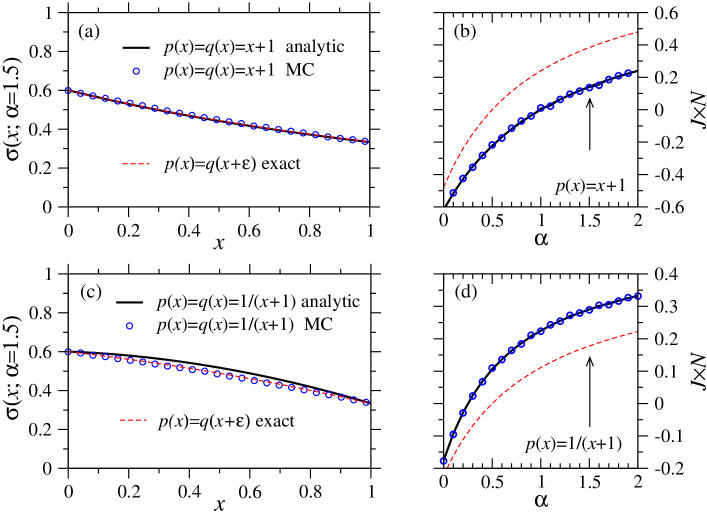
Figure 2: Densities and currents from analytic solutions of the Riccati equation and from simulations. (a) The density profile resulting from the linear hopping rate function $p(x)=q(x)=x+1$. Results from the analytic solution Eq. 18 (solid curve) and from Monte-Carlo simulations (circles) are shown. Also shown is the exact density for the purely diffusive case $p(x)=q(x+\varepsilon)=x+1$ (dashed curve). (b) Currents derived from both the analytic solution Eq. 19 (solid curve) and Monte-Carlo simulations (circles). Also shown for contrast is the exact current in the purely diffusive case (dashed curve). (c) The density profiles associated with the hopping rate function $p(x)=q(x)=1/(x+1)$. The solid, circled, and dashed curves correspond to analytic, Monte-Carlo, and exact diffusion (for $p(x)=q(x+\varepsilon)=1/(x+1)$) solutions. (d) Currents derived from both simulation and the analytic solution to Eq. 32. The arrows in (b) and (d) mark the value $\alpha=1.5$ used in plotting the density profiles shown in (a) and (c).

In Figs. 2, we plot (a) the densities and (b) the currents for the hopping rate profile $p(x)=q(x)=ax+b$ as a function of driving $\alpha$. The results of extensive Monte-Carlo simulations using the BKL continuous time algorithm [22], for a lattice of size $N=1000$, are also shown. Both analytic (in the $\varepsilon\rightarrow 0$ limit) and simulation results agree to a high degree of accuracy. In Figs. 2(c) and (d), we plot the densities and currents corresponding to the inverse hopping rate profile $p(x)=q(x)=a/(x+b)$. Here, the current also agrees well with the Monte-Carlo simulations. However, there is a small discrepancy between the densities from mean field theory and those from Monte-Carlo simulations. This discrepancy is not unexpected since correlations are neglected in mean field theory. Also shown for comparison are the densities and currents for the purely diffusive chain where $p(x)=q(x+\varepsilon)$. These densities (dashed curves) are very close to those corresponding to $p(x)=q(x)$, however, the diffusive currents are significantly different. By shifting the backward hopping rate function by $\varepsilon$, the density profile changes only slightly. However, since the steady-state currents scale as $\varepsilon$, small changes in boundary densities can lead to large relative differences in the steady-state currents.

5 Completely driven chain: $|p(x)-q(x)|\gg O(\varepsilon),\,0<x<1$

In this Section, we consider significantly different forward and backward hopping rates, and for simplicity, first assume $p(x)>q(x)$ for $0<x<1$. In this case, neither $P(x)$ nor $Q(x)$ is small, but Eq. 6 can be treated using singular perturbation theory and the appropriate implementation of density boundary layers. Suppose a boundary layer arises near $x\sim\varepsilon$. Rescaling $x=\varepsilon y$, we find

$${\mbox{d}\sigma(y)\over\mbox{d}y}=-JP(\varepsilon y)+Q(\varepsilon y)\sigma(y)(1-\sigma(y)).$$ (33)

Within the boundary layer, $y\sim O(1)$, $P(\varepsilon y)\approx P(0)$, and $Q(\varepsilon y)\approx Q(0)$. Equation 33 can be integrated to find the left inner solution

$$\sigma^{in}_{\ell}(y)={\sigma_{+}(0)(\sigma_{0}-\sigma_{-}(0))-\sigma_{-}(0)(\sigma_{0}-\sigma_{+}(0))e^{(\sigma_{-}(0)-\sigma_{+}(0))Q(0)y}\over\sigma_{0}-\sigma_{-}(0)-(\sigma_{0}-\sigma_{+}(0))e^{(\sigma_{-}(0)-\sigma_{+}(0))Q(0)y}},$$ (34)

where $\sigma_{\pm}(0)$ is also the outer solution to Eq. 33,

$$\sigma_{\pm}(x)={1\over 2}\pm{1\over 2}\sqrt{1-{4JP(x)\over Q(x)}},$$ (35)

evaluated as $x\rightarrow 0$. Of the two possible outer solutions, only $\sigma_{+}(0)$ can match the inner solution $\sigma^{in}_{\ell}(y\rightarrow\infty)$. The uniform solution with a density boundary layer at $x\sim\varepsilon$ is thus

$$\sigma_{\ell}(x)=\sigma_{\ell}^{in}(x/\varepsilon)+\sigma_{+}(x)-\sigma_{+}(x=0).$$ (36)

This solution automatically satisfies the boundary condition at $x=0$: $\sigma_{\ell}(0)=\sigma_{0}$. The current is determined by satisfying the boundary condition at $x=1$; and since $\sigma^{in}_{\ell}(y=1)\sim\sigma_{+}(0)$,

$$\begin{array}[]{rl}\sigma_{\ell}(1)\simeq&\displaystyle\sigma_{+}(1)={1\over 2}+{1\over 2}\sqrt{1-{4JP(1)\over Q(1)}}\\[13.0pt] \>=&\displaystyle\sigma_{N}={\delta+J\over\beta+\delta}.\end{array}$$ (37)

The only possible solution to Eq. 37 is

$$J={1\over 2}\left(\beta-\delta-{P(1)\over Q(1)}(\beta+\delta)^{2}\right)+{1\over 2}\sqrt{\left(\beta-\delta-{P(1)\over Q(1)}(\beta+\delta)^{2}\right)^{2}+4\beta\delta}.$$ (38)

In addition to this result, two other solutions to Eq. 33 exist. One with a boundary layer at $x\sim 1$, and another with boundary layers at both $x\sim\varepsilon$ and $x\sim 1$. If a boundary layer exists only at $x\sim 1$, only $\sigma_{-}(x)$ can match the inner solution near $x=1$ and the uniform the solution analogous to Eq. 36 is

$$\sigma_{r}(x)=\sigma_{r}^{in}(x/\varepsilon)+\sigma_{-}(x)-\sigma_{-}(x=1),$$ (39)

where

$$\sigma_{r}^{in}(x/\varepsilon)={\sigma_{+}(1)(\sigma_{N}-\sigma_{-}(1))-\sigma_{-}(1)(\sigma_{N}-\sigma_{+}(1))e^{(\sigma_{+}(1)-\sigma_{-}(1))Q(1)(1-x)/\varepsilon}\over\sigma_{N}-\sigma_{-}(1)-(\sigma_{N}-\sigma_{+}(1))e^{(\sigma_{+}(1)-\sigma_{-}(1))Q(1)(1-x)/\varepsilon}}.$$ (40)

In this case, the self-consistent current is found from $\sigma_{r}(0)=\sigma_{0}$:

$$J={1\over 2}\left(\alpha-\gamma-{P(0)\over Q(0)}(\alpha+\gamma)^{2}\right)+{1\over 2}\sqrt{\left(\alpha-\gamma-{P(0)\over Q(0)}(\alpha+\gamma)^{2}\right)^{2}+4\alpha\gamma}.$$ (41)

When both boundary layers exist, the outer solutions must match at at least one intermediate interior position $\sigma_{+}(x^{*})=\sigma_{-}(x^{*}),\,0\ll x^{*}\ll 1$. The corresponding uniform solution is

$$\sigma_{*}(x)=\bigg{\{}\begin{array}[]{c}\sigma_{\ell}(x)\quad 0\leq x\leq x^{*}\\[13.0pt] \sigma_{r}(x)\quad x^{*}\leq x\leq 1\end{array}$$ (42)

with corresponding maximal current

$$J_{max}={Q(x^{*})\over 4P(x^{*})}.$$ (43)

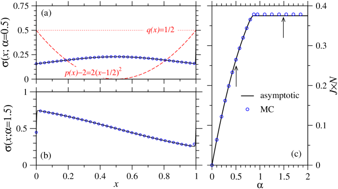
Figure 3: Densities and currents from asymptotic solutions of the Riccati equation and from simulations. Parameters used are $\varepsilon=1/1000$, $\beta=\gamma=1$, $\delta=0.5$, and $p(x)=2+2(x-1/2)^{2}>q(x)=1/2$. In all plots, the solid black curves correspond to asymptotic solutions of the mean field equations, while the blue circles correspond to results provided by Monte-Carlo simulations. (a) Asymptotic and simulation densities for $\alpha=0.5$. These parameters used render the system in a low density, entry rate-limited regime. (b) For $\alpha=1.5$, the system is in the maximal current phase ($J_{max}=3/8$), where boundary layers arise at both $x\approx 0$ and $x\approx 1$, and $x^{*}=1/2$. (c). The steady-state current as a function of $\alpha$. Given the other parameters used, the system transitions from a low density to a maximal current phase at $\alpha=5/6$. The parameters $\alpha=0.5,1.5$ used in plotting the densities in (a) and (b) are marked with arrows.

The solutions Eqs. 38, 41, and 43 are valid only in the parameter regimes where $J\leq Q(x^{*})/4P(x^{*})$ and $0\leq\sigma\leq 1$, and represent a generalization of the well-established three phase current structure arising in the constant $p,q$ PASEP [13, 14]. This three phase structure is preserved only if $p(x)-q(x)$ does not change sign on $x\in[0,1]$. Note that if $p,q$ are constant and $p-q>0$, the inner solutions are exact on $x\in[0,1]$ and we recover the known results for the PASEP [13, 14]. The mean field densities and currents for $p(x)=2+2(x-1/2)^{2}$ and $q=1/2$ are plotted in Figure 3, along with results from continuous-time Monte-Carlo simulations. The agreement is extremely good between the asymptotic mean field currents and simulation currents, suggesting that the basic physics of the three phase structure is preserved and that mean field theory provides exact, steady-state currents. The densities are also in good agreement, except in barely discernible region within the boundary layers where mean field and simulation derived densities differ. Note that there is also a slight discrepancy between mean field and simulation currents in the maximal current regime (Fig. 3c). The underestimation of the current by the mean field analysis results from the finite size of the rate-limiting region. Although $\varepsilon$ is small, and $p(x)$ is reasonably slowly varying, the rate limiting region at $x\approx 1/2$ is small enough for actual current (from MC simulations) to be noticeably greater than the asymptotic mean field result.

6 Opposing drifts: $|p(x)-q(x)|\gg O(\varepsilon)$ except at countable points $x_{0}$

Finally, consider the important class of hopping rates where $|p(x)-q(x)|\gg O(\varepsilon)$, except at certain points $x_{0}$ where $p(x)-q(x)$ crosses zero, like $Q(x)$ in the $\varepsilon\rightarrow 0$ limit. Examples of $p(x),q(x)$ with these properties are $p(x)=a+bx$, $q(x)=a+b(1-x)$ (where $x_{0}=1/2$), and periodic $p(x),q(x)$ such that $Q(x)$ oscillates above and below zero. Periodic hopping rates may arise during transport through pores with atomic periodicity. For example, periodic arrangements of atoms or molecules within the pore would impart a periodic potential on translocation of particles of the form $p(x)\propto\exp[(V(x)-V(x+\varepsilon))/k_{B}T]$ and $q(x)\propto\exp[(V(x)-V(x-\varepsilon))/k_{B}T]$, which are periodic if $V(x)$, the interaction potential as a function of the coordinate $x$ along the axis of the chain is itself periodic.

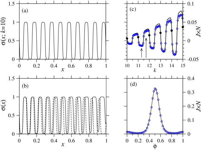
Figure 4: Densities and currents from solutions of the Riccati equation and from simulations for the periodic hopping rates modeled by Eq. 44. The parameters used are: $a=1$, $b=0.5$, $\alpha=1.5$, $\beta=\gamma=1$, $\delta=0.5$. (a) $p(x)$ (dashed), $q(x)$ (dotted), and the numerically solved density profile for $k=10,\phi=0$. (b) Numerically computed density profiles for $k=11.3,\phi=0$ (solid) and $k=11.7,\phi=0$ (dashed). (c) Numerically solved (solid) and simulation-derived (circles) steady-state currents as a function of $k$ ($\phi=0$). The arrows indicate $k=11.3,11.7$ used for generating the profiles in (b). Currents associated with integer values of $k$ are denoted by filled circles. (d) The current as a function of the phase difference $\phi$ between $p(x)$ and $q(x)$ for $k=12$.

Instead of specifying a detailed, molecular model for the hopping rates, we assume $p(x),q(x)$ to be functions that qualitatively capture the physics arising from periodic hopping rates. The qualitative dependence of the steady-state currents and densities should not depend upon the exact, quantitative forms chosen for the periodic hopping rates. Therefore, for simplicity, we assume:

$$\begin{array}[]{l}\displaystyle p(x)=a+b\sin^{2}(\pi kx)\\[13.0pt] \displaystyle q(x)=a+b\cos^{2}(\pi kx+\pi\phi),\end{array}$$ (44)

with $k>1$ and $a>b$. This functional form for the hopping rates captures the periodicity of the pore potential and allows for a phase difference $\phi$ between the forward and backward hopping rates. When $\phi=0$, $p(x)+q(x)=2a+b$, $P(x)=2/(2a+b)$, and the function $Q(x)=-2b\cos(2\pi kx)/(2a+b)$ crosses zero at points $x_{0}=(2n+1)/(4k)$. Despite this simplification, there is no analytic solution to Eq. 6, and we were unable to find approximations. Asymptotic analysis of the Riccati is also difficult due to the existence of multiple, interior boundary layers, and the fact that we must determine the boundary densities to $O(\varepsilon)$ in order to extract the current $J$. Moreover, numerical solutions to Eq. 6 are difficult to obtain for extremely small $\varepsilon$ since numerical errors build up as one integrates Eq. 6 from $x=0$ to $x=1$. Nonetheless, we compare currents and densities derived from numerics and continuous-time Monte-Carlo simulations.

Figures 4 show numerically computed ($\varepsilon=0.001$) and simulated ($N=1001$) densities and currents for periodic hopping rates Eq. 44. In Fig 4(a) are the functions $p(x),q(x)$, and the density profile for $k=10$ and $\phi=0$. Due to the oscillatory nature of $p(x)$ and $q(x)$, the densities are locally compressed and rarefied, rapidly jumping between $\sigma(x)=0$ and $\sigma(x)=1$. The numerically computed densities for noninteger $k$ are also shown in Fig. 4(b). Small changes in $k$ can cause large variations in the density near the $x=1$ boundary, causing dramatic changes in the current, as shown in Fig. 4(c). Fig 4(d) shows the sensitivity of the current to variations in the phase $\phi$. For clarity have shown only numerically computed density profiles: in our plots, densities found from simulations are nearly indiscernable from those found numerically. As in all other cases of slowly varying hopping rates, mean-field theory appears to yield exact steady-state currents. The agreement between numerical and simulated data is extremely good in Fig. 4(c), but the discrepancy increases as the number of hopping rate oscillations $k$ increases.

7 Summary and Conclusions

We have formulated the mean field approximation of a partially asymmetric exclusion process in the hydrodynamic limit in terms of the solution to the Riccati equation. This nonlinear equation can be solved in special cases and asymptotically analyzed in others. We compare numerical and analytical results with results from extensive, ($10^{9}-10^{1}0$ steps) continuous time Monte-Carlo simulations and find extremely good agreement for the steady-state particle currents. The numerical simulations fall well within the within the simulation error, typically $\lesssim 1\%$ and barely discernible in our plots. This agreement holds for all hopping rate profiles considered, provided they do not vary rapidly along the lattice. Moreover, although we have not proven that soutions to the Ricatti equations (Eqs. 6) yield exact currents, comparison of the numerical solutions for the current with those obtained from extensive continuous-time MC simulations shows a decreasing discrepancy as $\varepsilon/\ell\rightarrow 0$, provided sufficient long simulations are performed. Therefore, we conjecture that mean field approximations provide asymptotically exact steady-state currents as long as the hopping rate structure is smoothly varying in the thermodynamic ($N\rightarrow\infty$) limit.

The simulated densities, as expected, are quantitatively different from those obtained from the numeric or analytic solution of the Ricatti equation. Moreover, we find that the three-phase current structure of the PASEP is preserved when $p(x)>q(x)$. For cases where $|p(x)-q(x)|\leq O(\varepsilon)$ (pure diffusion and shifted diffusion), $J\sim\varepsilon$, but is sensitive to even slight shifts between the functions $p(x)$ and $q(x)$. The cases $p(x)=q(x)$ and $p(x)=q(x+\varepsilon)$ correspond to physically realizeable systems, yet yield very different results. When $p(x)$ and $q(x)$ vary periodically, as might be expected along a molecular channel constructed from a periodic array of atoms or molecules, the currents derived from solving Eq. 6 also appear to be exact, provided there are a large number of sites in each period.

Acknowledgments The authors are grateful for support from the US National Science Foundation through grants DMS-0206733 and DMS-0349195, and from the US National Institutes of Health through grant K25AI058672. JO was also supported by NIGMS Systems and Integrative Biology Training Grant 5T32GM008185. This research has been enabled by the use of WestGrid computing resources which are funded in part by the Canada Foundation for Innovation, Alberta Innovation and Science, BC Advanced Education, and the participating research institutions. WestGrid equipment is provided by IBM, Hewlett Packard, and SGI.

References

References

- [1] Nagel K and Schreckenberg M 1992 J. Physique I 2 2221-2229
- [2] Cheybani S, Kertesz J and Schreckenberg M 2000 Phys Rev E 63 016108
- [3] Karimipour V 1999 Phys. Rev. E59 205
- [4] Chou T 1998 Phys. Rev. Lett. 80 85-88
- [5] Chou T 1999 J. Chem. Phys. 110 606-615
- [6] MacDonald C T and Gibbs J H 1969 Bioploymers 7 707
- [7] Chou T 2003 Biophys. J. 85 755-773
- [8] Chou T and Lakatos G 2004 Phys. Rev. Lett. 93 198101
- [9] Vilfan A, Frey E and Schwabl F 2001 Europhys. Lett. 56 420-426
- [10] Schutz G and Domany E 1993 J. Stat. Phys. 72 277-296
- [11] Derrida B, Evans M R, Hakim V and Pasquier V 1992 J. Stat. Phys. 69 667-687
- [12] Derrida B 1998 Physics Reports 301 65-83
- [13] Sandow S 1994 Phys. Rev. E50 2660-2667
- [14] Essler F H and Rittenberg V 1996 J. Phys. A: Math. Gen. 29 3375-3407
- [15] Kolomeisky A B, Schutz G M, Kolomeisky E B and Straley J P 1998 J. Phys. A: Math. Gen. 31 6911-6919
- [16] Nagy Z, Appert C and Santen L 2002 J. Stat. Phys. 109 623
- [17] Kolomeisky A B 1998 J. Phys. A 31 1153-1164
- [18] Lakatos G, Chou T and Kolomeisky A B 2005 Phys. Rev. E 71 011103
- [19] Parmeggiani A, Franosch T and Frey E 2004 Phys. Rev. E 70 046101
- [20] Evans M R, Juh sz R and Santen L 2003 Phys. Rev. E 68 026117
- [21] The continuum definition of continuity, , yields the integration constant .
- [22] Bortz A B, Kalos M H and Lebowitz J L 1975 J. of Comp. Phys. 17 10-18