Glassy dynamics, aging and thermally activated avalanches in interface pinning at finite temperatures

Abstract

We study numerically the out-of-equilibrium dynamics of interfaces at finite temperatures when driven well below the zero-temperature depinning threshold. We go further than previous analysis by including the most relevant non-equilibrium correction to the elastic Hamiltonian. We find that the relaxation dynamics towards the steady-state shows glassy behavior, aging and violation of the fluctuation-dissipation theorem. The interface roughness exponent $\alpha\approx 0.7$ is found to be robust to temperature changes. We also study the instantaneous velocity signal in the low temperature regime and find long-range temporal correlations. We argue $1/f$-noise arises from the merging of local thermally-activated avalanches of depinning events.

The dynamics of interfaces in random media has received much attention, both theoretical and experimental, in the last decade. This is largely due to the interest in driven interfaces as models for nonlinear cooperative transport in many contexts, such as stochastic surface growth and kinetic roughening barabasi , magnetic flux lines in type-II superconductors scII , the motion of charge density waves gruner , propagation of fracture cracks bouchaud , fluid imbibition in porous media alava , etc. The competition between elastic interactions and quenched disorder leads to a rich behavior, which is not yet fully understood. A key macroscopic observable to look at is the average interface velocity $v$ as a function of the external driving force $f$. At zero temperature, quenched disorder tends to pin the interface and this leads to a depinning transition from a pinned phase ($v=0$) to a moving phase ($v>0$) at a critical value of the external driving force $f_{c}$. However, one particularly important question is how the system responds to this external forcing in the presence of non-negligible thermal fluctuations.

At finite temperatures, when the interface is driven well below the zero-temperature critical force $f_{c}(T=0)$, the interface velocity $v$ is extremely small. The interface then moves in bursts of activity, which are thermally activated and, in the steady state, the response of the system to a small external force exhibits glassy properties known as creeping creep . Experiments creep_exp and theoretical studies creep_theo have confirmed the existence the creep behavior. Theoretical approaches to this problem using mean-field or functional renormalization group techniques cugliandolo96 ; chauve ; balents ; schehr ; nattermann are usually valid in high dimensions and difficult to extend to one dimensional interfaces. More importantly, these approaches treat the dynamics of an elastic string in a random potential, i.e. interaction terms derive from an elastic energy $\mathcal{H}=(\nu/2)\int dx[\sqrt{(\nabla h)^{2}+1}+\Phi_{p}(x,h)]$ in a random pinning potential $\Phi_{p}$ in the small slopes limit $|\nabla h|\ll 1$. However, the elastic line approach gives a roughness exponent $\alpha\approx 1.2$ at the depinning transition, which leads to difficulties in the thermodynamic limit since interface fluctuations $\langle[h(x)-\overline{h}(x)]^{2}\rangle\sim L^{2\alpha}$ diverge and, indeed, the small slopes approximation breaks down rosso ; doussal .

Recent theoretical arguments have pointed out that a Kardar-Parisi-Zhang (KPZ) nonlinearity kpz may emerge from anisotropy of the disorder tang and/or from higher order terms in an elastic expansion rosso ; doussal . Also, recent developments in imaging technology have allowed to directly visualize the boundary between the vortex invaded and the vortex free (Meissner) regions in superconductors. In a series of nice experiments Surdeanu et al. surdeanu recently measured the temporal and spatial correlations of these fronts for a YBa₂Cu₃O_7-x superconductor. They reported interfaces that exhibited scale-invariant kinetic roughening with exponents consistent with KPZ dynamics. Similar results were later obtained in Ref. vlasko for thin Nb superconductor films. These theoretical and experimental results make evident the importance of understanding the effect of thermal fluctuations on pinned interfaces when the interaction between degrees of freedom contains nonequilibrium contributions, like the KPZ nonlinearity.

In this Letter we study the relaxation towards the steady state of an interface locally pinned by a disordered background. Our study includes the most relevant KPZ non-equilibrium correction to the elastic energy. We focuss on the interface dynamics well below the depinning transition, when only temperature can locally detach the interface. We find that the system very slowly relaxes (creeping) to a steady-state. During the relaxation regime the system exhibits aging and violation of the fluctuation-dissipation theorem. The roughness exponent of the string is found to be $\alpha\approx 0.7$ at short scales and robust to changes in temperature. Remarkably, the instantaneous velocity signal exhibits long-range temporal correlations. We argue $1/f$-noise arises from the merging of local thermally-activated avalanches of depinning events.

We consider a 1D line described by a single-valued function $h(x,t)$, giving the transversal position $h$ of the front from the $h=0$ axis at time $t$. The front is moving through a heterogeneous medium, which can be described by a quenched disorder $\eta(x,h)$ and the interface obeys the equation of motion:

$$\partial_{t}h=\nu\,\nabla^{2}h+\lambda\,(\nabla h)^{2}+\sqrt{T}\,\xi(x,t)+\sigma\,\eta(x,h)+f,$$ (1)

where $\xi(x,t)$ is a gaussian white noise with zero mean and unit variance describing the thermal fluctuations at temperature $T$, $\nu$ is the elastic constant, and the KPZ nonlinearity $\lambda\,(\nabla h)^{2}$ gives the most relevant nonequilibrium correction to the equilibrium elastic energy. We only consider here the case of non-correlated gaussian disorder so that $\langle\eta(x,y)\eta(x^{\prime},y^{\prime})=\delta(x-x^{\prime})\,\delta(y-y^{\prime})$ and $\langle\eta(x,y)\rangle=0$.

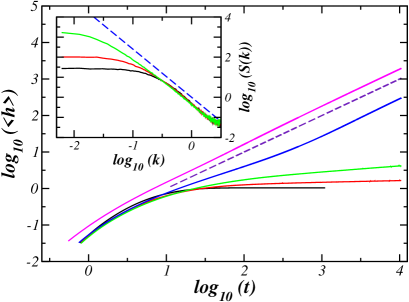
Figure 1: (Color online) Average height as a function of time for the nonlinear equation. The different curves correspond from bottom to top to the temperatures $T=0,0.01,0.04,0.16$ and $0.64$. In the inset, the spatial power spectra of the interfaces for the three lowest temperatures (colors match in both graphs). The dashed lines have slope $1$ in the main plot and slope $-(2\alpha+1)=-2.4$ in the inset.

Interface scaling.-

We have carried out extensive numerical simulations of the Langevin equation of motion (1). To solve (1) numerically we discretized $h(x,t)$ along the $x$ direction with lattice spacing $\Delta x=1$ and used a stochastic Euler scheme to integrate the equation of motion with periodic boundary conditions. The constants $\nu$ and $\sigma$ can be scaled out and without lose of generality we have set $\nu=\sigma=1$. All the results reported in the following were obtained for an integration time step $\Delta t=0.01$, which was enough to guaranty stability of the numerical scheme and $\Delta t$-independence of the numerical results. We are interested in the fully nonlinear regime, thus, for the system sizes we used (up to $L=2046$), the strength of the nonlinear term is set to $\lambda=1$. Our results do not depend on $\lambda$, as far as it is large enough to allow the nonlinearity to fully operate well before saturation is reached. For comparison we have also studied the usual elastic regime for $\lambda=0$.

Simulations at $T=0$ revealed that the depining transition takes place at $f_{c}(T=0,\lambda=1)=0.36\pm 0.01$ and $f_{c}(T=0,\lambda=0)=0.99\pm 0.01$ for the nonlinear and linear models, respectively. A more precise determination of the critical thresholds is not required since we are interested in the dynamics of the system well below the critical point. In the following, unless otherwise stated, we will always be driving the system with external forces $f(\lambda=1)=0$ and $f(\lambda=0)=0.1$, well below the critical threshold. We now focuss on the effects of varying the external temperature $T$ when the system is in the zero-temperature pinned phase.

We always start our simulation with a flat interface $h=0$ and then let the system evolve at a given temperature $T$. We monitor the average height $\langle\overline{h}\rangle$ from which the interface velocity can be obtained in the long times limit $v\equiv\lim_{t\to\infty}\langle\overline{h}\rangle/t$.

Initially, as may be seen in Figure 1, the front advances very fast. The interface moves through the quenched disorder and progressively gets locally trapped at more and more pinning sites. The duration of this transient is system size independent and relatively short. After that initial outburst, the interface begins relaxation towards the steady state. The latter is characterized by a constant velocity. The time span of the relaxation process strongly depends on temperature, increasing very dramatically at low $T$. During relaxation, the average height displays a nonlinear growth in time, $\langle\overline{h}\rangle\sim t^{\gamma(T)}$, characteristic of the creeping regime. The actual value of $\gamma(T)$ decays rapidly with decreasing $T$, being the average height at very low $T$ compatible with a logarithmic growth.

This singular dynamics of the average height during the creeping regime imposes constrains upon the evolution of the interface width. Since $w(t,L)\sim t^{\alpha/z}$ cannot grow faster than the height $\langle\overline{h}\rangle\sim t^{\gamma}$, we have $\alpha/z\leq\gamma(T)$. Simulations show that the value of the roughness exponent $\alpha\approx 0.7$ remains essentially constant at low temperatures. In the inset of Figure 1 we plot the structure factor $S(k,t)=\langle\hat{h}(k,t)\hat{h}(-k,t)\rangle$ at long times $t=10^{4}$ for three different temperatures $T=0,0.01$ and $0.04$ (where $\hat{h}$ is the the Fourier transform of the interface height in a system of lateral size L, with $k$ being the spatial frequency in reciprocal space). The inset clearly shows that (i) after long times $10^{4}$ the interface has not yet reached a steady state, (ii) the interface is scale-invariant $S(k,t)\sim k^{-(2\alpha+1)}$ at short scales $k\gg t^{-1/z}$, and (iii) the roughness exponent $\alpha$ does not depend on temperature. This in turn implies that it is the dynamic exponent $z$ the one changing with temperature (since $\alpha/z\leq\gamma(T)$). This is made more evident as $T\to 0$, when dynamics is dramatically slowed down and $z$ suffers a significative increment.

Aging.-

Ultra-slow relaxation towards the steady state indicates typical out of equilibrium glassy features in the system, in particular the existence of aging–namely, the breakdown of the time translation invariance symmetry cugliandolo96 ; yoshino ; cugliandolo97 . In order to study aging in our system we compute the two-times connected correlation function

$$\Gamma(t,t_{w})=\langle\overline{[h(x,t)-\langle h\rangle(t)]\,[h(x,t_{w})-\langle h\rangle(t_{w})]}\rangle.$$ (2)

If the system ages, $\Gamma(t,t_{w})$ must be a function of both $t$ and $t_{w}$, and not only of their difference $t-t_{w}$. We follow the standard procedure, which closely mimics what can be done in real experiments. The interface is evolved at some very high fixed temperature (we typically used $T=4$ for the nonlinear equation and $T=36$ for the linear case) to anneal the system until the stationary state is reached. Then, when the system is in the steady-state, the temperature is suddenly decreased to the desired measuring level $T$. This sets up the system out of equilibrium and the time counter is started, $t=0$, at the freezing event. We then monitor the relaxation dynamics by measuring $\Gamma(t,t_{w})$. Typical $\Gamma(t,t_{w})$ curves for a set of waiting times $t_{w}$ are shown in Figure 2 for a external temperature $T=0.04$ and $0.49$ for the nonlinear and linear cases, respectively. Both the nonlinear and the linear equations show clear aging during relaxation towards the steady state similarly to other glassy systems.

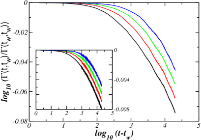
Figure 2: (Color online) Connected correlation as a function of the time difference $t-t_{w}$. The main graph is for the nonlinear equation at $T=0.04$ and $t_{w}=250,500,1000$ and $2000$ from left to right. In the inset, the same plot but for the linear equation, at $T=0.49$ and the same set of $t_{w}$ values.

Fluctuation-dissipation violation.-

Another important aspect of glassy dynamics is the way in which the fluctuation-dissipation relation is broken. At equilibrium, the susceptibility is linearly related to the spatial correlations of the conjugated variable. A modification for slowly evolving out of equilibrium systems has been recently proposed by Cugliandolo, Kurchan and Peliti cugliandolo97 , through the generalized response function

$$R(t,t_{w})=\frac{X[\Gamma]}{T}\,\frac{\partial\Gamma(t,t_{w})}{\partial t_{w}},$$ (3)

where $R(t,t_{w})=\langle\overline{\delta h(x,t)/\delta f(x,t_{w})}\rangle$, i.e., the response of the conjugated variable (the interface height in our case) at a time $t$ to the application of a local external field (the driving force $f$ in our case) at the same position $x$ at a previous time $t_{w}$. $X[\Gamma]$ is a functional that can vary between two asymptotic constant values, either it takes value one (for scales that are already in the stationary regime) or $X[\Gamma]\to X_{\infty}$ (for those scales that are still out of equilibrium).

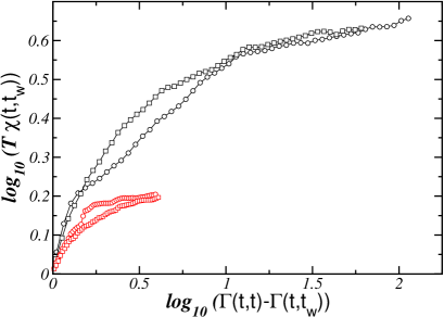
Figure 3: (Color online) Parametric representation of the susceptibility as a function of the connected correlations for the nonlinear model with $T=0.01$ (black curves) and $0.02$ (red ones). The waiting times in both cases are $t_{w}=500$ (circles) and $t_{w}=1000$ (squares).

Numerically, it is more convenient to study the susceptibility, defined as $\chi(t,t_{w})=\int_{t_{w}}^{t}ds\,R(t,s)$, instead of the response function $R(t,t_{w})$. The reason being that the computation of $\chi(t,t_{w})$ does not require the introduction of an instantaneous spike-like perturbation in the external field and, in addition, the integration in time implies that the external field operates during a period of time making the estimation of its effects much easier to detect. We integrate $R(t,s)$ in Eq. (3) in the variable $s$ and obtain

$$\chi(t,t_{w})=\frac{X[\Gamma]}{T}\,[\Gamma(t,t)-\Gamma(t,t_{w})].$$ (4)

In order to check whether the fluctuation-dissipation relation is broken during relaxation in our system, we use a similar numerical setup as before. We anneal the system by heating at very high temperatures until a steady-state is reached, then the temperature is decreased and that event marks the time origin $t=0$. After a waiting time $t_{w}$, we run in parallel two copies A and B of the interface. Copy A is then driven with constant force $f^{\rm A}(x,t)=f^{\rm A}$ as before, and copy B is driven with a slightly different local driving force $f^{\rm B}(x,t)=f^{\rm A}+\delta f(x)$, where $\delta f(x)$ is a small uncorrelated random field which takes at random the values $\pm\epsilon$ with equal probability. The susceptibility can then be approximated by $\chi(t,t_{w})\sim\langle\overline{(h^{\rm B}(x,t)-h^{\rm A}(x,t))\,\delta f(x)}\rangle/|\epsilon|$. In Figure 3, parameteric plots with the susceptibility as a function of $\Gamma(t,t)-\Gamma(t,t_{w})$ are shown for the nonlinear equation ($\lambda=1$) and for different temperatures. The fluctuation-dissipation theorem is clearly violated, again akin to observations in other glassy systems.

Thermally activated avalanches.-

Finally, we pay attention to the dynamics of avalanches at finite temperatures in the nonlinear model Eq. (1). Avalanches in forced superconductors have attracted much attention altshuler ; aval , but little is known about avalanche dynamics at a finite $T$. $\overline{h}(t)$ data (not shown) for a single disorder realization have a dented and devil staircase-like appearance caused by the stick–slip motion associated with avalanches triggered by a local thermally-activated depinning event. We monitor the avalanche dynamics in our system by looking at the temporal correlations of the average velocity signal $v(t)=\overline{\partial_{t}h}(t)$ well below $f_{c}(T=0)$. In Figure 4, we plot the spectral density $\mathcal{S}(w)=\langle|\hat{v}(w)|^{2}\rangle$, averaged over disorder realizations. The velocity signal $v(t)$ shows long-range temporal correlations. In the low-frequency limit we observe a power-law decay $\mathcal{S}(w)\sim w^{-\theta}$ with a temperature-dependent exponent $\theta(T)$ ranging from uncorrelated noise $\theta\sim 0$ (at very low temperatures) to long-range correlations $1.0<\theta(T)<1.2$ for temperatures in the range $0.05<T<0.20$. For even higher temperatures, $T\geq 0.25$, velocity spectra clearly show a crossover to a different power-law decay with exponent $\theta(T)\approx 0.30$, which then remains unaltered when temperature is further increased. The latter regime corresponds to a free-moving interface in the KPZ universality class, which velocity-fluctuation spectra is known to diverge as $1/w^{\theta}$ at low frequencies, where $\theta=(d+4)/z-3$ in $d+1$ dimensions krug . In $d=1$ one then finds that $\theta=1/3$ in good agreement with our numerical results at high temperatures where the interface is freely moving with a finite displacement velocity. We obtained similar results for the linear case ($\lambda=0$), where $\theta\sim 1$ in the intermediate temperatures regime, and the crossover to $w^{0}$ for the highest temperatures, as expected for the linear equation krug .

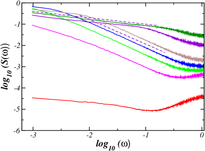
Figure 4: (Color online) Spectral densities of the velocity signal for the nonlinear equation ($\lambda=1$). Temperatures are $T=0.01$, $0.09$, $0.1225$, $0.16$, $0.25$, $1$ and $2.25$ from bottom to top. The straight lines are guide for the eye and have a slope $-0.3$ and $-1.16$ respectively.

This change in the temporal correlations of the velocity signal at high enough temperatures can be pinned down to the existence of thermally activated avalanches of depinning events. When the interface is driven well below $f_{c}$ at finite temperatures, uncorrelated avalanches of typical size $\xi$ are triggered all over the front. At very low temperatures thermally activated avalanches are very unlikely and localized events, disjoint and uncorrelated to one another, giving rise to a typical flat spectrum ($\theta\sim 0$) of the velocity signal. However, at higher temperatures we expect more sites to detach from disorder and so more local avalanches to occur. Avalanches can overlap and merge to give rise to a larger avalanche, eventually covering a macroscopic region of the interface. This leads to bursts of spatially connected moving events and, consequently, long-range temporal correlations ($\theta\sim 1$) in the interface velocity fluctuations. This can be seen in Figure 4 for $0.09\leq T\leq 0.16$. The higher the temperature, the more likely a site gets depinned, triggering a local avalanche of depinning events of size $\xi$. Eventually, at high enough temperatures ($T\approx 0.25$ in Figure 4) all the pinning sites are overcome by the merging of local avalanches that can extend across the whole system freeing the interface from the disorder. Further increasing the temperature above that point will not affect the dynamics since temperature is high enough to overcome local pinning and the depinning transition is actually wiped out. In this regime the interface is described by the KPZ dynamics and $w^{-1/3}$ velocity-fluctuation spectra.

- (1) A. -L. Barabási, and H. E. Stanley, Fractal Concepts in Surface Growth, Cambridge Univ. Press, Cambridge (1995).
- (2) G. Blatter et al., Rev. Mod. Phys. 66, 1125 (1994); L. F. Cohen and H. J. Jensen, Rep. Prog. Phys. 60, 1581 (1997).
- (3) G. Grüner, Rev. Mod. Phys. 60, 1129 (1998).
- (4) E. Bouchaud, J. Phys. Condens. Matter 9, 4319 (1997).
- (5) M. Alava, M. Dube, M. Rost, Adv. Phys. 53 83 (2004).
- (6) L. B. Ioffe and V. M. Vinokur, J. Phys. C 20, 6149 (1987); T. Nattermann, Europhys. Lett. 4, 1241 (1987); V. M. Vinokur, M. C. Marchetti, and L. -W. Chen, Phys. Rev. Lett. 77, 1845 (1996); S. Scheidl and V. M. Vinokur, Phys. Rev. Lett. 77, 4768 (1996).
- (7) S. Lemerle et. al., Phys. Rev. Lett. 80, 849 (1998); F. Cayssol et. al., Phys. Rev. Lett. 92, 107202 (2004); T. Tybell et. al., Phys. Rev. Lett. 89, 097601 (2002).
- (8) P. Chauve, T. Giamarchi, and P. Le Doussal, Phys. Rev. B 62, 6241 (2000); A. B. Kolton, A. Rosso, and T. Giamarchi, Phys. Rev. Lett. 94, 047002 (2005).
- (9) L. F. Cugliandolo, J. Kurchan, and P. Le Doussal, Phys. Rev. Lett. 76, 2390 (1996).
- (10) P. Chauve, P. Le Doussal, and K. Wiese, Phys. Rev. Lett. 86, 1785 (2001).
- (11) L. Balents and P. Le Doussal, Phys. Rev. E 69, 061107 (2004).
- (12) G. Schehr and P. Le Doussal, Phys. Rev. Lett. 93, 217201 (2004).
- (13) T. Nattermann et al., Phys. Rev. Lett. 87, 197005 (2001).
- (14) A. Rosso and W. Krauth, Phys. Rev. Lett. 87, 187002 (2001).
- (15) P. Le Doussal et al., Phys. Rev. Lett. 96, 015702 (2006).
- (16) M. Kardar, G. Parisi, and Y. -C. Zhang, Phys. Rev. Lett. 56, 889 (1986).
- (17) L. -H. Tang, M. Kardar, and D. Dhar, Phys. Rev. Lett. 74, 920 (1995).
- (18) R. Surdeanu et al., Phys. Rev. Lett. 83, 2054 (1999).
- (19) V. K. Vlasko-Vlasov et al., Phys. Rev. B 69, 140504(R) (2004).
- (20) H. Yoshino, Phys. Rev. Lett. 81, 1493 (1998).
- (21) L. F. Cugliandolo, J. Kurchan, and L. Peliti, Phys. Rev. E 55, 3898 (1997).
- (22) A. B. Kolton et al., Phys. Rev. Lett. 89, 227001 (2002).
- (23) E. Altshuler and T. H. Johansen, Rev. Mod. Phys. 76, 471 (2004).
- (24) H. J. Jensen, Phys. Rev. Lett. 64, 3103 (1990); K. E. Bassler and M. Paczuski, Phys. Rev. Lett. 81, 3761 (1998).
- (25) J. Krug, Phys. Rev. A, 44, R801 (1991).