Reorganization asymmetry of electron transfer in ferroelectric media and principles of artificial photosynthesis

Abstract

This study considers electronic transitions within donor-acceptor complexes dissolved in media with macroscopic polarization. The change of the polarizability of the donor-acceptor complex in the course of electronic transition couples to the reaction field of the polar environment and the electric field created by the macroscopic polarization. An analytical theory developed to describe this situation predicts a significant asymmetry of the reorganization energy between charge separation and charge recombination transitions. This result is proved by Monte Carlo simulations of a model polarizable diatomic dissolved in a ferroelectric fluid of soft dipolar spheres. The ratio of the reorganization energies for the forward and backward reactions up to a factor of 25 is obtained in the simulations. This result, as well as the effect of the macroscopic electric field, is discussed in application to the design of efficient photosynthetic devices.

I Introduction

Electron transfer (ET) reaction is a basic elementary step in photoinduced charge separation occurring in both natural and artificial photosynthesis. The fundamental mechanism behind the conversion of light energy into the energy of a charge-separated state is illustrated in Figure 1. Optical excitation $h\nu$ of the donor unit, D$\to$D^∗, within the donor-acceptor complex, D–A, lifts the energy level of the donor to create conditions for the photoinduced charge separation step, D^∗–A $\to$ D⁺–A^-. Charge separation is generally an activated transition. The activation barrier, according to the Marcus-Hush theory,Marcus:93 can be obtained from the equilibrium free energy gap between the final and initial ET states, $\Delta F_{0}$, and the free energy $\lambda$ required to reorganize the nuclear degrees of freedom (reorganization free energy). When the equilibrium free energy of the acceptor is below the free energy of the donor by the amount of free energy $\lambda$, the charge separation transition is activationless. Such an activationless transition is often fast and efficient, but it requires loosing the energy $\lambda$ from the photon energy $h\nu$. Increasing the energetic efficiency of photosynthesis therefore demands $\lambda$ to be as low as possible. It is often assumed that an important role played by the hydrophobic protein matrix in facilitating ET in natural photosynthesis is to screen highly polar aqueous environment and to reduce $\lambda$.

Once the charge-separated state has been created, it needs to be sufficiently long-lived to be used for energy storage. A mechanism often suggested to be of primary importance in natural systems is the use of a sequence of activationless ET steps to move the electron away from the primary donor. Each activationless step $i$ lowers the system energy by $\lambda_{i}$ thus resulting in the overall low energetic efficiency of the photosynthetic unit. The reaction competing with photoinduced charge separation is the normally highly exothermic return electron transfer to the ground D–A state. The classical reaction path then goes through the relatively high activation barrier in the inverted ET region predicted by the Marcus-Hush theory (point “C” in Figure 1).Marcus:93 However, the system avoids this activated path by nearly activationless transfer to a vibrationally excited state, D–A(v), of the electronically ground donor-acceptor complex (dashed line in Figure 1). The vibrational energy is subsequently released to heat through vibrational relaxation ($v\to 0$ in Figure 1).

The design an optimization of a sequence of activationless ET reactions requires a very precise molecular tuning, which is hard to achieve in synthetic systems despite some significant progress achieved in this field in recent years.Wasielewski:92 ; Moore:93 It is therefore desirable to search for mechanisms of reducing the rate of return ET in molecular photosynthesis with the goal of achieving higher quantum yield for the charge-separated state. According to the current understanding of radiationless transitions in molecules,BixonJortner:99 an efficient way to reduce the return rate would be to move the reaction into the normal region of ET.

The electronic states D^∗–A and D–A are distinct and, in principle, the charge-recombination transition D⁺–A${}^{-}\to$ D–A can be characterized by a pair of parabolas with the curvatures different from those of the charge-separation transition D^∗–A $\to$ D⁺–A^-. In the reactions classification adopted here we label transition D^∗–A $\to$ D⁺–A^- as charge separation and transition D⁺–A^- $\to$ D–A as charge recombination. Backward transitions at each step are not considered as separate steps in the reaction mechanism. When the photoexcitation energy is kept constant, shifting the recombination reaction into the normal region would require increasing the curvature of the charge-recombination parabolas (dash-dotted lines in Figure 1), i.e. lowering the reorganization energy. The inverted-region activated state C then shifts to the normal-region activated state C^′ in Figure 1.

It is easy to realize the pitfall of the picture shown in Figure 1. The separation of the minima of two dash-dotted parabolas must be equal, in the Marcus-Hush theory, to twice the reorganization energy, which is clearly violated once the curvature is increased without corresponding shift of the parabolas. Therefore, the goal of bringing the recombination reaction to the normal region can be realized only within models extending beyond the Marcus-Hush picture of equal-curvature parabolas. On needs flexibility, built into the model, that would allow decoupling of the Stokes shift from the curvatures. The use of parabolic free energy surfaces with different curvatures, as was suggested by Kakitani and Mataga,Kakitani:85 is prohibited by the requirement of energy conservation. When the energy gap between the donor and acceptor energy levels is taken for the reaction coordinate, the free energy surfaces of the initial, $F_{1}(X)$, and final, $F_{2}(X)$, ET states are connected by the linear relation established by WarshelHwang:87 and TachiyaTachiya:89

$$F_{2}(X)=F_{1}(X)+X$$ (1)

The parabolic surfaces with different curvatures clearly violate this requirement and, therefore, cannot be used for the modeling of ET reactions. The problem can be resolved within a three-parameter model of ET free energy surfacesDMjcp:00 which allows different reorganization energies and, at the same time, does not violate eq 1. The free energy surfaces $F_{i}(X)$ are then necessarily non-parabolic.

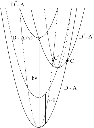
Figure 1: Energetics of photoinduced electron transfer involved in natural and artificial photosynthesis. The charge-separated state D⁺–A^- is placed below the photo-excited state D^∗–A by the reorganization energy $\lambda$ to ensure activationless transition. The dashed line indicates the vibrationally excited electronic ground state for which the recombination transition D⁺–A${}^{-}\to$D–A does not require an activation barrier. The dash-dotted lines mark the free energy surfaces of states D⁺–A^- and D–A with the reorganization energy four times lower than the value of $\lambda$ used to draw the free energy surfaces shown by the solid lines. C and C^′ indicate the classical transition states.

Once different reorganization energies are allowed within a theory of free energy surfaces, one needs to address the following major question: What would be a mechanism resulting in dramatic changes of reorganization energies between charge separation and charge recombination reactions? A question relevant to studies of natural photosynthesis is the following: Is the role of the protein matrix can be reduced to providing a low dielectric constant or there are some other properties of proteins beneficial for high efficiency of natural photosynthesis? Note that shifting the transition point from C to C^′ requires a very significant change in the reorganization energy (four times decrease in Figure 1). The possibility of different equilibrium-point curvatures of the two ET free energy surfaces has been actively pursued in the last decades by computer simulations searching for the effects of non-linear solvation on ET.Hwang:87 ; Kuharski:88 ; Marchi:93 ; Yelle:97 ; Hartnig:01 ; DMjcp2:04 However, essentially in all reports, the difference in reorganization energies between the initial and final ET states has never come close to the magnitude that would dramatically change the mechanism of charge recombination.

In this paper, we address the problem of reorganization asymmetry by considering ET reactions in polarizable donor-acceptor complexes immersed in polarization anisotropic media. A part of the motivation for this approach comes from studies of bacterial photosynthesis. The protein matrix in natural bacterial reaction centers is highly anisotropic with the electric field amounting $\simeq 10^{7}$ V/cm.Steffen:94 On the other hand, the primary pair is highly polarizable with the polarizability change upon photoexcitation about 800–1100 ų.Middendorf:93 Since bacteriochlorophyll cofactors are much less polarizable,Kjellberg:03 primary charge separation occurs with a large negative polarizability change. On a more fundamental level, polarizability change in the course of ET leads to very significant reorganization asymmetry, as follows from both analytical theoriesDMjpca:99 and computer experiment.DMjacs:03 ; DMjpca:04 The asymmetry arising from the coupling of changing polarizability to the solvent recation field is by far the largest achieved so far in computer simulations thus promising the desired alteration of the energetics of photosynthetic reactions.

In Section II, we present an analytical model of ET free energy surfaces when both the polarizability and the dipole moment of the donor-acceptor complex change in the course of ET. The donor-acceptor complex is immersed in a polar medium which, in addition to usual polar response, is characterized by a macroscopic electric field. In order to mimic high electric fields present in molecular systems (thin films, proteins, etc.), we use a polar model fluid capable of producing ferroelectric order (Section III). The ordered phase is obtained by Monte Carlo (MC) simulations. The possibility of ferroelectric order in bulk polar fluids is still actively debated in the literature,Wei:92 ; Zhang:95 ; Morozov:03 and it has been suggested that boundary conditions employed in the simulation protocol significantly affect the possibility of creation of the macroscopically polar phase.Wei:93 For our current purpose, this subject is not relevant since we are mostly interested in reactions in condensed phases with macroscopic electric fields strong enough to influence properties of electronic transitions. Whether the macroscopic polar order is stabilized by surface effects or some other reasons is not central to our study. On the other hand, ferroelectrics and ordered polar films may be used as solvents for ET reactions. The present analysis then directly applies to such systems. We return to discussing the role of reorganization assymetry in improving the efficiency of phtosynthesis in Section IV.

II Energetics of electron transfer

II.1 Model

Consider a donor-acceptor complex immersed in a medium with a nonzero macroscopic electric field $\mathbf{F}$. The complex has the dipole moments $\mathbf{m}_{0i}$ and polarizabilities $\bm{\alpha}_{0i}$ in two electronic states, $i=1,2$. These states are coupled to nuclear fluctuations in the solvent and are “dressed” with the field of the electronic solvent polarization following adiabatically the changes in the charge distribution within the complex. Because of the electronic polarization, the dipole moments and polarizabilities are different from their gas phase values $\mathbf{m}_{0i}$ and $\bm{\alpha}_{0i}$:DMjpca:99

$$\mathbf{m}_{i}=\left[\mathbf{1}-2\bm{\alpha}_{0i}\cdot\mathbf{a}_{e}\right]^{-1}\cdot\mathbf{m}_{0i}$$ (2)

and

$$\bm{\alpha}_{i}=\left[\mathbf{1}-2\bm{\alpha}_{0i}\cdot\mathbf{a}_{e}\right]^{-1}\cdot\bm{\alpha}_{0i}$$ (3)

Here, $\mathbf{a}_{e}$ is the linear response function such that the free energy of solvation of dipole $\mathbf{m}_{0}$ by the electronic solvent polarization (subscript “e”) is $\mathbf{m}_{0}\cdot\mathbf{a}_{e}\cdot\mathbf{m}_{0}$. Once the electronic degrees of freedom have been adiabatically eliminated, the electronic energy levels of the charge-transfer complex are affected by the microscopic nuclear field $\mathbf{R}_{n}$ (nuclear reaction field, subscript “n”) and the macroscopic field $\mathbf{F}$ of the solvent:DMjpca:99

$$E_{i}[\mathbf{R}_{n}]=I_{i}^{\text{np}}-\mathbf{m}_{i}\cdot(\mathbf{R}_{n}+\mathbf{F})-\frac{1}{2}(\mathbf{R}_{n}+\mathbf{F})\cdot\bm{\alpha}_{i}\cdot(\mathbf{R}_{n}+\mathbf{F})$$ (4)

Here $I_{i}^{\text{np}}$ are the energies of the ET complex which include the gas-phase energies and free energies of solvation by the solvent electronic polarization expressed as a sum of induction and dispersion solvation components.

The system Hamiltonian

$$H_{i}[\mathbf{R}_{n}]=E_{i}[\mathbf{R}_{n}]+H_{B}[\mathbf{R}_{n}]$$ (5)

is the sum of energies $E_{i}[\mathbf{R}_{n}]$ and the solvent bath Hamiltonian $H_{B}$. The Gaussian (linear response) approximation is adopted for the latter

$$H_{B}[\mathbf{R}_{n}]=\frac{1}{4}\mathbf{R}_{n}\cdot\mathbf{a}_{n}^{-1}\cdot\mathbf{R}_{n}$$ (6)

where $\mathbf{a}_{n}$ is the linear response function of the solvent nuclear polarization. In the following, for simplicity, we will assume collinear dipole moments $\mathbf{m}_{i}$ and the polarizability changing its value only along the direction of the dipole moment. We will also assume that the solute polarizability increases for the $1\to 2$ transition, i.e., $\Delta\alpha=\alpha_{2}-\alpha_{1}>0$. These approximations allow us to consider $\mathbf{a}_{n}$ as a scalar with the only non-zero projection along the solute dipole. We will also define the scalar $F_{m}$ as the projection of the external field $\mathbf{F}$ on the direction of the solute dipole moment. The consideration of a more general case does not present fundamental difficulties.DMjpca:99

II.2 Free energy surfaces

The classical Hamiltonian $H_{i}[\mathbf{R}_{n}]$ in eq 5 can be used to build the free energy surfaces of ET along the reaction coordinate associated with the fluctuating donor-acceptor energy gap required to reorganize the nuclear degrees of freedom

$$X=\Delta H[\mathbf{R}_{n}]=H_{2}[\mathbf{R}_{n}]-H_{1}[\mathbf{R}_{n}]$$ (7)

The free energy surfaces for the initial ($i=1$) and final ($i=2$) ET states are obtained by constrained integration over the nuclear reaction field

$$e^{-\beta F_{i}(X)}=A\int\delta(X-\Delta H[\mathbf{R}_{n}])e^{-\beta H_{i}[\mathbf{R}_{n}]}d\mathbf{R}_{n},$$ (8)

where $A$ is used to account for the units of the field $\mathbf{R}_{n}$ and $\beta=1/k_{\text{B}}T$.

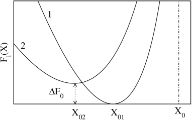
Figure 2: Free energy surfaces of ET $F_{i}(X)$ for the initial ($i=1$, “1”) and final ($i=2$, “2”) ET states. Shown in the plot are the free energy minima $X_{0i}$, the free energy gap $\Delta F_{0}=F_{02}-F_{01}$, and the upper boundary $X_{0}$ for the reaction coordinate $X$.

The Gaussian integral in eq 8 can be taken exactly with the result

$$F_{i}(X)=-\kappa_{i}X-\beta^{-1}\ln\left[\frac{\sinh\chi(X)}{\chi(X)}\right]$$ (9)

where

$$\chi(X)=2\beta\sqrt{\kappa_{i}^{3}\lambda_{i}(X_{0}-X)}$$ (10)

The parameters in eqs 9 and 10 are related to the properties of the polarizable donor-acceptor complex and the polar solvent by the following set of equations. The parameters $\kappa_{i}$ are

$$\kappa_{i}=\left(2a_{n}f_{ni}\Delta\alpha\right)^{-1}$$ (11)

The parameter $f_{ni}$ in eq 11 is responsible for the enhancement of the effective solute dipole by the interaction of the solute polarizability with the nuclear reaction field (cf. to eqs 2 and 3)

$$f_{ni}=(1-2a_{n}\alpha_{i})^{-1}$$ (12)

Further,

$$X_{0}=I_{2}^{\text{np}}-I_{1}^{\text{np}}-\Delta mF_{m}-\frac{1}{2}\Delta\alpha F_{m}^{2}+\frac{(\Delta m+\Delta\alpha F_{m})^{2}}{2\Delta\alpha}$$ (13)

is the boundary of the fluctuation band of the reaction coordinate $X$ (Figure 2). The requirement $X<X_{0}$ implicit in the definition of $\chi(X)$ is eq 10 does not allow the energy gap fluctuations to exceed $X_{0}$. Finally, $\lambda_{i}$ in eq 10 is the solvent reorganization energy

$$\lambda_{i}=a_{n}f_{ni}\left[\Delta m+\Delta\alpha(R_{i}+F)\right]^{2}$$ (14)

where $\Delta m=m_{2}-m_{1}$ and reaction field $R_{i}$ is

$$R_{i}=2a_{n}f_{ni}m_{i}$$ (15)

The function $\chi(X)$ in eq 9 does not carry index specifying the ET state because of the relation connecting the parameters of the two ET states:

$$\kappa_{1}^{3}\lambda_{1}=\kappa_{2}^{3}\lambda_{2}$$ (16)

In addition, the parameters $\kappa_{1}$ and $\kappa_{2}$ are related by the additivity constant

$$\kappa_{1}-\kappa_{2}=1$$ (17)

The free energy surfaces defined in the range $X<X_{0}$ are non-parabolic, as is depicted in Figures 2 and 3. Each of them passes through the minimum at $X=X_{0i}$ defined by the condition

$$dF_{i}(X)/dX\bigg{|}_{X=X_{0i}}=0$$ (18)

This equation can be reduced to the algebraic equation for $\chi(X)$ which always has a non-zero solution

$$\chi\coth\chi-1=(2\beta\kappa_{i}^{2}\lambda_{i})^{-1}\chi^{2}$$ (19)

The solution is simplified when $\chi_{0i}=\chi(X_{0i})\gg 1$. One then gets

$$X_{0i}=X_{0}-\kappa_{i}\lambda_{i}$$ (20)

and the free energy at the minimum is

$$F_{0i}=-\kappa_{i}X_{0}-\kappa_{i}^{2}\lambda_{i}$$ (21)

In this limit, the second derivatives taken at the position of the minima define the two solvent reorganization energies, as is the case in standard formulations of ET theories

$$\frac{d^{2}F_{i}(X)}{dX^{2}}\Bigg{|}_{X=X_{0i}}=\frac{1}{2\lambda_{i}}$$ (22)

Note that from eq 21 the fluctuation boundary $X_{0}$ is related to the free energy gap $\Delta F_{0}=F_{02}-F_{01}$ and two reorganization energies by the relation

$$X_{0}=\Delta F_{0}+\kappa_{2}^{2}\lambda_{2}-\kappa_{1}^{2}\lambda_{1}$$ (23)

Taken together, eqs 9–23 provide an exact model for the free energy surfaces of ET (Figure 2) based on three thermodynamic parameters, $\lambda_{1}$, $\lambda_{2}$, and $\Delta F_{0}$. The present model thus extends the two-parameter Marcus-Hush theory, based on the assumption $\lambda_{1}=\lambda_{2}$,Marcus:93 to three-parameters space. In view of the connection between $\kappa_{1}$ and $\kappa_{2}$ (eq 17), one of them can be considered as the non-parabolicity parameter:

$$\kappa=\kappa_{1}=\left(1-\sqrt[3]{\frac{\lambda_{1}}{\lambda_{2}}}\right)^{-1}$$ (24)

In terms of the solute polarizability and the solvent nuclear response function, the non-parabolicity parameter becomes

$$\kappa=\frac{1-2a_{n}\alpha_{1}}{2a_{n}\Delta\alpha}$$ (25)

Because of the choice $\Delta\alpha>0$ adopted here, $\lambda_{1}<\lambda_{2}$ and $\kappa_{i}>0$.

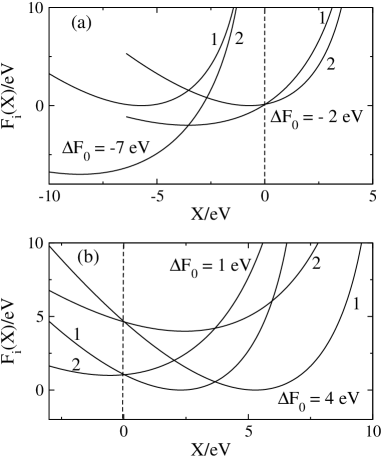
Figure 3: Free energy surfaces $F_{i}(X)$ at $\lambda_{1}=1$ eV and $\lambda_{2}=2$ eV. The free energy gap $\Delta F_{0}$ is: $-2$ eV and $-7$ eV in (a) and 1 eV and 4 eV in (b). The free energy surfaces corresponding to $\Delta F_{0}=-7$ eV in (a) do not have the classical crossing point $X=0$ indicated by the dashed lines in both panels.

It is easy to prove that $F_{i}(X)$ from eq 9 obey the energy conservation requirement given by eq 1. Note that the present model exhausts the space of thermodynamic parameters available for the description of ET reactions. Only three thermodynamic parameters, free energy gap between the minima and second cumulants of the fluctuations around the minima, are allowed by the two-state nature of the problem. Any extension of the theory for ET free energy surfaces beyond the present level will require non-equilibrium parameters to be involved.

The requirement of thermodynamic stability of the polarization fluctuations limits the range of possible values of the reaction coordinate, $X\leq X_{0}$. The reaction coordinate boundary $X_{0}$ is shown by the dash-dotted line in Figure 2. There is no singularity of $F_{i}(X)$ at $X=X_{0}$ and the free energies $F_{i}(X)$ are infinite at $X>X_{0}$. For reaction coordinates sufficiently far from $X_{0}$, the free energy surfaces can be conveniently re-written in the form

$$F_{i}(X)=F_{0i}+\kappa_{i}\left[\sqrt{X_{0i}+\kappa_{i}\lambda_{i}-X}-\sqrt{\kappa_{i}\lambda_{i}}\right]^{2}$$ (26)

When the reorganization energies $\lambda_{i}$ are close to each other, the non-parabolicity parameter $\kappa$ in eq 24 tends to infinity and one obtains the standard Marcus-Hush parabolas by expanding eq 26 in $1/\kappa$. From eq 26, the activation energy of ET is

$$\Delta F_{i}=F_{i}(0)-F_{0i}=\kappa_{i}\left[\sqrt{X_{0i}+\kappa_{i}\lambda_{i}}-\sqrt{\kappa_{i}\lambda_{i}}\right]^{2}$$ (27)

II.3 Qualitative results

The three-parameter model predicts some novel results regarding the dependence of the reaction rates on the free energy gap (energy gap law). In order to illustrate them, we will consider the transition from the activated normal region to the activated inverted region through the activationless transition for the forward reaction $1\to 2$ and the backward reaction $2\to 1$ while maintaining $\lambda_{1}<\lambda_{2}$ and the definition of the free energy gap as $\Delta F_{0}=F_{02}-F_{01}$ (Figure 2). Our analysis here assumes $\chi_{0i}\gg 1$, which holds for most cases of interest. For the forward reaction $1\to 2$, the transition from the normal to the inverted region is marked by the equation $X_{01}=0$, which corresponds to a line in the space of parameters $\lambda_{2}/\lambda_{1}>1$ and $\Delta F_{0}/\lambda_{1}$ (Figure 4):

$$\Delta F_{0}/\lambda_{1}=\kappa(\kappa+1)-(\kappa-1)^{2}(\lambda_{2}/\lambda_{1})$$ (28)

The line shrinks into the point $\Delta F_{0}/\lambda_{1}=\pm 1$ in the Marcus-Hush limit of equal reorganization energies (marked as “MH” in Figure 4).

Lowering the free energy gap in the inverted region for the forward reaction 1$\to 2$ leads to a new region of ET absent in the Marcus-Hush theory. When the boundary of the band of allowed energy gaps $X_{0}$ crosses the transition state $X=0$, the classical crossing point of two free energy surfaces falls outside the range of allowed reaction coordinates. No crossing of free energy surfaces $F_{i}(X)$ is then possible ($\Delta F_{0}=-7$ eV in Figure 3(a)), and the classical reaction channel is closed, $\Delta F_{1}=\infty$. The reaction occurs only through vibrational excitations of the final ET state 2 effectively lowering the free energy gap. The transition to this new region, which may be called “quantum tunneling region” ($\Delta F_{1}=\infty$ in Figure 4(a)), is marked by the line $X_{0}=0$ is the space of parameters $\lambda_{2}/\lambda_{1}$ and $\Delta F_{0}/\lambda_{1}$.

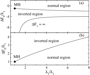
Figure 4: Normal and inverted region in the space of parameters $\Delta F_{0}/\lambda_{1}$ and $\lambda_{2}/\lambda_{1}$. Shown are the results for the forward reaction $1\to 2$ (a) and for the backward reaction $2\to 1$ (b). The quantum tunneling region with $\Delta F_{1}=\infty$ in (a) is separated from the inverted region by the condition $X_{0}=0$, which puts the classical crossing point outside the range of reaction coordinates $X<X_{0}$ allowed by the condition of thermodynamic stability. The dots labeled as “MH” refer to the Marcus-Hush limit in which the transition from the normal to inverted region is given by the conditions: $\Delta F_{0}/\lambda=-1$ for $1\to 2$ and $\Delta F_{0}/\lambda=1$ for $2\to 1$.

Due to the asymmetry of the free energy surfaces for $\lambda_{2}/\lambda_{1}>1$, the normal region spans different ranges of $\Delta F_{0}$ for positive and negative free energy gaps. Figure 4 shows a broader normal-range ET for $\Delta F_{0}>0$. This observation suggests that the goal of bringing the exothermic recombination reaction to the normal region (Figure 1) is easier to achieve when the reorganization energy of the charge-separated state D⁺–A^- is much higher than the reorganization energy of the ground state D–A (see Discussion).

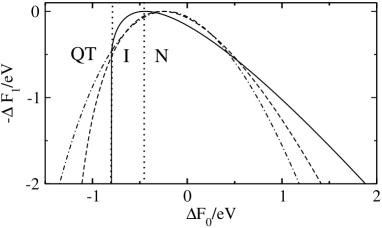
Figure 5: Energy gap law for the reaction 1$\to$2 ($\lambda_{1}<\lambda_{2}$) at $\lambda_{1}=0.2$ eV and $\lambda_{2}=0.25$ eV (dash-dotted line), $\lambda_{2}=0.4$ eV (dashed line), and $\lambda_{2}=2$ eV (solid line). The dotted lines separates the normal (N), inverted (I), and quantum tunneling (QT) regions for $\lambda_{2}=2$ eV.

The overall classical energy gap law (no vibrational excitations) for the present model is illustrated in Figure 5. With increasing the ratio of the reorganization energies $\lambda_{2}/\lambda_{1}$, the bell-shaped dependence of $-\Delta F_{1}$ on $\Delta F_{0}$ becomes increasingly shallow in its right wing with positive energy gaps $\Delta F_{0}>0$, approaching the linear energy gap law $\Delta F_{1}\propto\Delta F_{0}$. On the other hand, the approach of the fluctuation boundary $X_{0}$ to the transition point $X=0$ squeezes the left wing narrowing the inverted region of ET.

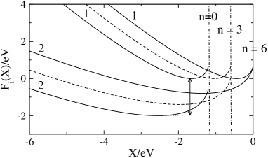
Figure 6: Inverted-region reaction $1\to 2$ with $\lambda_{1}=0.2$ eV, $\lambda_{2}=1.0$ eV, and $\Delta F_{0}=-2$ eV (shown by the vertical arrow). Classical transitions between vibrationally ground-state surfaces are forbidden by the condition $X_{0}<0$. The dashed surfaces obtained for $n=3$ do not contribute to the Franck-Condon weighted density of states since $X_{0}+n\hbar\omega_{v}<0$ for $n=3$. For $n\geq 6$, $X_{0}+n\hbar\omega_{v}>0$ ($\hbar\omega_{v}=0.2$ eV) and these vibronic transitions contribute to the overall density of states. The dash-dotted lines indicate the fluctuation boundary $X_{0n}$ at $n=0$ and $n=3$; $X_{0n}=0$ at $n=6$.

The quantum vibronic excitations of the donor-acceptor complex can be included in the standard way by considering the Franck-Condon weighted density of states (FCWD) as a Poisson-weighted sum over the vibronic excitations leading to $n$ vibrational quanta in the final ET state.BixonJortner:99 For instance, for the forward reaction one gets

$$\mathrm{FCWD}(X;1\to 2)=e^{-S}\sum_{n=0}^{\infty}\frac{S^{n}}{n!}e^{-\beta F_{1n}(X)}$$ (29)

Here, $S=\lambda_{i}/\hbar\omega_{v}$ is the Huang-Rhys factor, $\omega_{v}$ is the characteristic vibrational frequency, and $F_{1n}(X)$ is obtained from eq 9 by replacing there $X_{0}$ with

$$X_{0n}=X_{0}+n\hbar\omega_{v}$$ (30)

The Arrhenius factor for the rate constant can be obtained (within a factor) by putting $X=0$ in eq 29. Since the thermodynamic stability of the nuclear fluctuations requires $X<X_{0n}$, only terms corresponding to $X_{0n}>0$ in eq 30 will contribute to the sum in eq 29. This fact implies a modification of the standard picture of the FCWD made of a Poisson-weighted sum of vibronic transitions. Vibronic transitions with $n<-X_{0}/(\hbar\omega_{v})$ will not contribute to the FCWD as is illustrated by $n=0$ and $n=3$ in Figure 6. Only starting from vibrational excitation number making $X_{0n}$ positive ($n=6$ in Figure 6) will a given vibronic transition contribute to the FCWD. This fact will result in a greater asymmetry of emission lines making the red-side wing of an optical band more shallow than the blue-side wing.

III Electron transfer in ferroelectrics

Equation 14 for the solvent reorganization energies of a polarizable donor-acceptor complex is the central result of the formal theory relevant to our discussion of reorganization anisotropy in ferroelectrics. Equation 14 predicts that the polarizability change $\Delta\alpha$ couples to the macroscopic and local (reaction) fields to modify the change in the solute dipole moment in the course of electronic transition. Depending on the relative signs of $\Delta m$ and $\Delta\alpha(R_{i}+F_{m})$, the solute polarizability may increase or decrease the solvent reorganization energy compared to the non-polarizable limit. The main question in this regard is whether the term $\Delta\alpha(R_{i}+F_{m})$ can achieve a magnitude comparable to $\Delta m$. Below, we address this question by MC simulations of a model donor-acceptor diatomic in a dipolar ferroelectric solvent. Here, we first provide some relevant estimates.

The mean-field Weiss theory of spontaneous dipolar polarizationZhang:95 relates the macroscopic field in a sample of aligned dipoles $m$ to their number density $\rho$ as

$$F=(4\pi/3)\rho m$$ (31)

The term $\Delta\alpha F_{m}/m$ at $\rho^{*}=\rho\sigma^{3}=0.7$ is then $\simeq 3\Delta\alpha/\sigma^{3}$ when the solute dipole is aligned with the macroscopic field, $\sigma$ is the solvent diameter. The polarizability change may vary substantially between different donor-acceptor units, but the ground-state polarizability is close to $\sigma_{0}^{3}/16$ for many molecular systems ($\sigma_{0}$ is the effective solute diameter). If $\Delta\alpha$ is of the same order of magnitude as the ground-state polarizability, $3\Delta\alpha/\sigma^{3}$ scales as $(\sigma_{0}/\sigma)^{3}$. For example, for primary charge separation in Rhodobacter sphaeroids, $\Delta m\simeq 53$ D.Bixon:95 If we accept $\sigma=2.87$ Å and $m=1.83$ D for water and $\Delta\alpha\simeq 800$ Å,Middendorf:93 then $\Delta m/m\simeq 29$ and $\Delta\alpha F_{m}/m\simeq 100$ thus resulting in comparable order-of-magnitude contributions from the change in the permanent charges and from the interaction of the polarizability change with the non-homogeneous electric field. In addition, from the estimate of the local electric field of the protein matrix at the position of the primary pairSteffen:94 $F\simeq 10^{7}$ V/cm, the induced dipole $\Delta\alpha F\simeq 27$ D is also comparable to $\Delta m\simeq 53$ D.

III.1 Simulations

A fluid of soft spheres is known to spontaneously form a ferroelectric liquid phase when conducting boundary conditions are employed in the simulation protocol.Wei:92 This system was used here to model a disordered phase with a molecular-scale macroscopic polarization coupled to the electronic states of the donor-acceptor complex. Two sets of simulations have been carried out. The fluid of soft dipolar spheres was simulated in the first set in order to establish the range of parameters for which ferroelectric phase can be detected. This was followed by the second set of simulations in which polarizable donor-acceptor complex was dissolved in the ferroelectric liquid.

MC simulations of the pure solvent employed NVT ensemble of $N=500$ particles in a cubic simulation cell at the reduced density of $\rho^{*}=\rho\sigma^{3}=0.7$. The molecules are interacting with the potential

$$v(12)=4\epsilon\left(\sigma/r_{12}\right)^{12}-\mathbf{m}_{1}\cdot\mathbf{T}_{12}\cdot\mathbf{m}_{2}$$ (32)

where $\epsilon$ is the repulsion energy, $\sigma$ is the diameter, $\mathbf{m}_{j}$ is the dipole moment with the magnitude $m$, $\mathbf{T}_{12}=\nabla_{1}\nabla_{2}r_{12}^{-1}$ is the dipolar tensor, and $r_{12}=|\mathbf{r}_{1}-\mathbf{r}_{2}|$. Simulations were done at $\beta\epsilon=1.35$ and varying reduced dipole $(m^{*})^{2}=\beta m^{2}/\sigma^{3}$. Periodic boundary conditions and reaction-field correction for dipolar interactions with conducting boundary conditionsAllen:96 have been employed. The length of simulations was $10^{6}$ cycles long far from the transition point and up to $10^{7}$ cycles long close to the transition to ferroelectric phase.

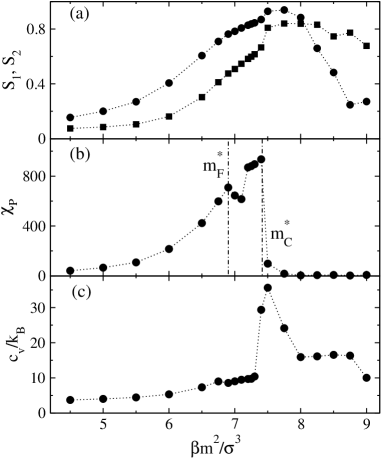
Figure 7: First ($S_{1}$, circles) and second ($S_{2}$, squares) order parameters of the fluid of dipolar soft spheres vs $\beta m^{2}/\sigma^{3}$ (a). Also shown are the dipolar susceptibility $\chi_{P}$ (b) and constant-volume heat capacity $c_{V}$ (c). The dotted lines connect the simulation points. The dash-dotted lines in (b) indicate the points of phase transition to ferroelectric fluid ($m_{F}^{*}$) and fcc crystal ($m_{C}^{*}$).

Transition to ferroelectric phase was monitored by calculating the first-order, $S_{1}$, and second-order, $S_{2}$, parameters (Figure 7(a)). The first-order (ferroelectric) parameter quantifies the spontaneous polarization

$$S_{1}=M/Nm$$ (33)

where $\mathbf{M}$ is the total dipole moment of the solvent. The second-order (nematic) parameter is defined as the largest eigenvalue of the ordering matrixAllen:96

$$\mathbf{Q}=(2N)^{-1}\sum_{j}(3\mathbf{\hat{e}}_{j}\mathbf{\hat{e}}_{j}-\mathbf{1})$$ (34)

where $\mathbf{\hat{e}}_{j}=\mathbf{m}_{j}/m$.

Both order parameters change smoothly with $m^{*}$ and do not allow a reliable identification of the transition point.Weis:05 Susceptibilities, which are expected to show sharp spikes at the points of phase transition,Binder:92 are better indicators. Indeed, the dielectric susceptibility

$$\chi_{P}=(\beta/V)\langle(\delta\mathbf{M})^{2}\rangle$$ (35)

shows the first peak at $(m_{F}^{*})^{2}=6.9$ and the second peak at $(m_{C}^{*})^{2}=7.5$ (Figure 7(b)), where $V$ in eq 35 is the solvent volume. The heat capacity

$$c_{V}=3/2+\beta^{2}\langle(\delta E)^{2}\rangle/N$$ (36)

on the contrary, shows only a little bump at $m^{*}_{F}$ and a strong peak at $m^{*}_{C}$ (Figure 7(c)), where $E$ in eq 36 is the total energy of the fluid. The order parameters also show weak discontinuities at $m_{C}^{*}$. The examination of the density structure factors reveals that the system is in the liquid state below $m^{*}_{C}$ and crystallizes into an fcc lattice at this value of the reduced dipole. The point $m^{*}_{F}$ corresponds to the transition to a ferroelectric liquid. Note that the value of $m^{*}_{F}$ obtained here is very close to that predicted by a linear extrapolation of the phase transition line recently reported by WeisWeis:05 for dipolar hard spheres.

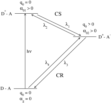
Figure 8: Charges and polarizabilities of the donor-acceptor complex in three states involved in photoinduced charge separation (CS) and charge recombination (CR).

The ferroelectric liquid at $(m^{*})^{2}=7.0$, $\rho^{*}=0.7$, and $\beta\epsilon=1.35$ was used to study the dependence of the solvent reorganization energy on solute polarizability. In these simulations, a donor-acceptor diatomic made of two hard fused spheres of diameters $\sigma_{0}/\sigma=1.5$ with the center-to-center separation $d/\sigma=0.6$ was inserted in the center of a cubic simulation cell containing $N=500$ soft dipolar particles at $\rho^{*}=0.7$. Two opposite charges $q_{0}^{*}=\beta|q_{0}|/\sigma=10$ where placed at the centers of two spheres in the charge-separated state thus producing the dipole moment $m_{02}=d|q_{0}|$. The induced point dipole moment $\mathbf{p}_{0i}=\mathbf{\hat{e}}_{0}\alpha_{0i}R_{i}$, caused by the dipolar polarizability $\alpha_{0i}$ and reaction field $R_{i}$, is placed at the midpoint of the line connecting the two centers of the diatomic. $\mathbf{p}_{0i}$ is aligned along the unit vector $\mathbf{\hat{e}}_{0}$ along the same line. The solute induced dipole was equilibrated to each instantaneous configuration of the solvent by iteration algorithm (more details on the simulation protocol are given in ref DMjpca:04, ). Ewald sums with conducting boundary conditionsAllen:96 were used to calculate the solute-solvent electrostatic interactions.

Some complications arise from the fact that the director, $\mathbf{\hat{d}}=\mathbf{M}/Nm$, fluctuates in the simulations. In real liquid crystals, fluctuations of the macroscopic director occur on the time-scale of microseconds to seconds,Vertogen:88 much slower than orientational motions of molecular solutes. The director, therefore, does not fluctuate on the time-scale of the reaction. In order to account for this hierarchy of relaxation times, the simulation protocol was set up to keep the orientation of the donor-acceptor complex fixed relative to the director. The initial configuration was created by inserting a sphere of diameter $\sigma_{0}$ into the soft dipolar solvent followed by a short, $5\times 10^{3}$ cycles, equilibration run designed to establish the director $\mathbf{\hat{d}}$. The two spheres making the diatomic were then pulled apart at a given angle to the director and this angle was adjusted after each cycle over the $N$ solvent molecules. The data were collected from simulation runs of the length $6\times 10^{5}-1.2\times 10^{6}$ cycles. In the present simulations, the long axes of the diatomic was always aligned with the director in such a way that the charge-transfer dipole $\Delta\mathbf{m}_{0}$ is always parallel to the macroscopic field $\mathbf{F}$.

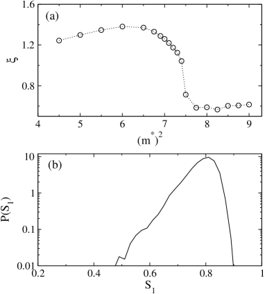
Figure 9: The linear response parameter $\xi$ from eq 40 (a) and the distribution function of the ferroelectric order parameter (b) obtained from MC simulations at $(m^{*})^{2}=7.0$, $\beta\epsilon=1.35$, and $\rho^{*}=0.7$. The dotted line in (a) connects the simulation points.

III.2 Energetics of photoinduced electron transfer

We have followed the basic design of photoinduced ET outlined in Figure 1 and detailed in terms of charges and polarizabilities in Figure 8. It is assumed that the donor-acceptor complex has no appreciable dipole moment and polarizability in its ground state ($q_{0}=0$, $\alpha_{g}=0$). Photoexcitation of the donor to state D^∗–A lifts the polarizability to $\alpha_{01}>0$ but does not substantially change the charge distribution, $q_{0}=0$. Both the charge distribution and polarizability change upon charge separation resulting in D⁺–A^- state ($q_{0}>0$, $\alpha_{02}>0$). Because of the coupling of the polarizability to the reaction field $R_{i}$ and the macroscopic electric field $F_{m}$ (eq 14), the reorganization energies will differ for forward and backward electronic transitions for both the charge separation and charge recombination steps of the reaction mechanism. Therefore, we need four reorganization energies, $\lambda_{1}$ and $\lambda_{2}$ for charge separation and $\lambda_{3}$ and $\lambda_{4}$ for charge recombination (Figure 8).

Table 1: Energetic parameters (eV) of the charge separation reaction (Figure 8) in which $\alpha_{01}$ is varied and $\alpha_{02}/\sigma^{3}=0.2$ is kept constant; $\beta q_{0}/\sigma=10$ in the charge-separated state.

$\alpha_{01}/\sigma^{3}$	$\lambda_{1}$	$\lambda_{2}$	$\Delta X_{0}$	$\Delta X_{0}$
0.2	0.324	0.456	0.817	0.770
0.3	0.344	0.371	0.750	0.715
0.4	0.373	0.295	0.706	0.665
0.5	0.477	0.229	0.704	0.666
0.6	0.587	0.171	0.665	0.647
0.7	0.761	0.123	0.612	0.640
0.8	1.314	0.083	0.645	0.733

The reorganization energies were calculated from MC configurations as second cumulants of the solute-solvent interaction potential.DMjpca:04 The polarizability of the photoexcited state $\alpha_{01}$ was varied at constant $\alpha_{02}/\sigma^{3}=0.2$ for charge separation and the polarizability of the charge-transfer state $\alpha_{02}$ was varied at $\alpha_{g}=0$ for charge recombination. Tables 1 and 2 and Figure 10 summarize the forward and backward reorganization energies for charge-separation and charge-recombination reactions along with the Stokes shift

$$\Delta X_{0}=X_{01}-X_{02}$$ (37)

From eq 20, the Stokes shift becomes

$$\Delta X_{0}=\kappa(\lambda_{2}-\lambda_{1})-\lambda_{2}$$ (38)

The Stokes shift in eq 37 is equivalent to the difference of absorption and emission maxima due to eq 1. Equation 38 also applies to the Stokes shift defined in terms of two first spectral moments

$$\Delta X_{0}=\langle X\rangle_{1}-\langle X\rangle_{2}$$ (39)

in the limit $\kappa_{i}\sqrt{\beta\lambda_{i}}\gg 1$.

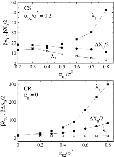
Figure 10: Reorganization energies and the Stokes shifts for the charge separation (CS) and charge recombination (CR) reactions (Figure 8) vs polarizability of the photoexcited state $\alpha_{01}$ (CS) and the polarizability of the charge-separated state $\alpha_{02}$ (CR); $q_{0}^{*}=10$, $\alpha_{g}=0$.

The direct comparison of the results of simulations to the three-parameter model discussed in Section II is complicated by the narrow range of solvent dipoles for which ferroelectric phase can be detected. The close proximity of two phase transition points makes the statistics of polarization fluctuations non-Gaussian, in contrast to the Gaussian approximation adopted in eq 6. There are several indications of significant deviations from the Gaussian statistics. The ratio

$$\xi=-\langle v_{ss}\rangle/\beta\langle(\delta v_{ss})^{2}\rangle$$ (40)

is equal to one ($\xi=1$) when polarization fluctuations are Gaussian (linear response approximation).DMjcp1:99 Here, $\langle v_{ss}\rangle$ is the average electrostatic interaction energy of a liquid particle with the rest $N-1$ particles in the liquid and $\langle(\delta v_{ss})^{2}\rangle$ is the variance of this electrostatic interaction. As is seen from Figure 9(a), this parameter is higher than one in the paraelectric phase and drops sharply at the transition to the ferroelectric phase. In addition, the distribution of macroscopic polarization $M$ in the simulation box is non-Gaussian. A shoulder seen in Figure 9(b) points to the importance of a $\propto M^{4}$ term in the polarization functional such as that present in the Landau theory of phase transitions.Vertogen:88

In terms of solvation properties, in the absence of polarizability change of the solute, $\Delta X_{0}/2$ should be equal to $\lambda=\lambda_{1}=\lambda_{2}$. The first lines in Tables 1 and 2 correspond to exactly this situation. The difference between two reorganization energies, as well as deviations of both of them from $\Delta X_{0}/2$ is another indication of the non-Gaussian statistics of the solvent polarization leading to non-linear solvation. Despite these complications, the direct calculations of the Stokes shift from simulations compare semi-quantitatively to the results of applying eq 38 (Tables 1 and 2). The analytical model developed in Section II.2, therefore, captures the basic thermodynamics of ET with markedly different reorganization energies.

Table 2: Energetic parameters (eV) of the charge recombination reaction (Figure 8) for which $\alpha_{02}$ is varied and $\alpha_{g}=0$ is kept constant; $\beta q_{0}/\sigma=10$ in the charge-separated state.

$\alpha_{02}/\sigma^{3}$	$\lambda_{3}$	$\lambda_{4}$	$\Delta X_{0}$	$\Delta X_{0}$
0.0	0.369	0.279	0.649	0.642
0.2	0.654	0.284	0.911	0.871
0.3	1.115	0.287	1.115	1.051
0.4	1.466	0.290	1.466	1.352
0.5	2.270	0.293	2.270	1.728
0.6	2.562	0.296	2.562	2.357
0.7	3.240	0.299	3.240	2.928
0.8	7.466	0.303	4.079	3.446

IV Discussion

The basic design of an artificial photosynthetic device, as advances by Meyer and co-workers,Huynh:04 ; Acevedo:05 is shown in Figure 11. It anticipates the creation of ordered arrays where donors and acceptors are connected to catalytic sites where high-energy reactions can occur (e.g., splitting of water or reduction of carbon dioxide to carbohydrates). This design requires efficient separation of the electron and the hole. Unless this separation is achieved by high mobility of each charge in molecular arraysHoertz:05 or in valence and conduction bands of a semiconductor,Lewis:05 high branching ratio between charge separation and charge recombination is required at each step of productive charge transfer to facilitate the redox reactions which are normally significantly slower than ET steps.

Figure 11: Reaction center model.Huynh:04 ; Acevedo:05 The unit C is photoexcited to obtain the electron from donor D and transfer it to acceptor A. The recombination rates $k_{r}$ at each stage should be sufficiently low to allow normally slow catalytic reduction (Ox${}_{1}\to$Red₁) and oxidation (Red${}_{2}\to$Ox₂) reactions to occur.

The model presented here offers some novel opportunities in terms of varying the parameters of ET reactions and activation barriers. The model emphasizes the coupling of the solute polarizability change, achieved in the course of electronic transition, to the electric field at the position of the donor-acceptor complex. The electric field has two components, the reaction field of the polar environment $R_{i}$ and the macroscopic field $F_{m}$. The coupling of the overall field $R_{i}+F_{m}$ to the polarizability change creates the effective dipole moment change of the donor-acceptor complex (eq 14)

$$\Delta m_{\text{eff},i}=\Delta m+\Delta\alpha(R_{i}+F_{m})$$ (41)

The reaction field $R_{i}$, which depends on the electronic state of the donor-acceptor complex, is responsible for the distinction between the forward and backward reorganization energies, $\lambda_{1}\neq\lambda_{2}$ and $\lambda_{3}\neq\lambda_{4}$ as is shown in Figure 10 and listed in Tables 1 and 2. Note that the asymmetry in the reorganization energies up to a factor of 25 obtained in our simulations (Table 2) is the largest ever observed in either computer or laboratory experiment.

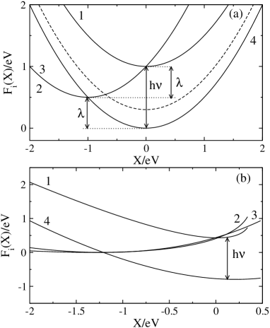
Figure 12: Free energy surfaces of photoinduced ET in the Marcus-Hush picture (a) and in the present model with different reorganization energies (b). The free energy surfaces are plotted against the reaction coordinate corresponding to the energy gap between the charge-separated and photoexcited states. The parameters are chosen to show the activationless pathway from the photoexcited state 1 to the charge-separated state 2 and from 2 to the ground state 3. The free energy surfaces 2 and 3 coincide in the Marcus-Hush picture, but are distinct in the present model. In (a) the dashed line indicates the free energy surface for the normal-region charge recombination when energetic efficiency is below 50%; $h\nu$ indicates the energy of photoexcitation. The reorganization energies are: $\lambda=1$ eV (a) and $\lambda_{1}=0.2$ eV, $\lambda_{2}=2.0$ eV, $\lambda_{3}=1.0$ eV, and $\lambda_{4}=0.5$ eV (b).

A note on the dual nature of the reorganization energy is relevant here. The reorganization energy for each ET state is calculated on the configurations of the solvent in equilibrium with the donor-acceptor complex in that given state. Therefore, the reorganization energy carries information about a particular electronic state of the donor-acceptor complex. On the other hand, the value that is being averaged is the change in the interaction potential, which is a characteristic of a given transition. As a result of this duality, the electronic charge-separated state of the donor-acceptor complex D⁺–A^- can be characterized by two, generally unequal, reorganization energies $\lambda_{2}$ and $\lambda_{3}$ reflecting transitions to two different electronic states, photoexcited and ground.

In the present picture, all reorganization energies $\lambda_{1}$, $\lambda_{2}$, $\lambda_{3}$, and $\lambda_{4}$ are allowed to be different, producing reach energetics of photoinduced charge separation and charge recombination. The difference in scenarios for photoinduced ET in the Marcus-Hush model and in the present formulation is illustrated in Figure 12. The plots show the free energy surfaces vs the reaction coordinate corresponding to the energy gap $X$ between the charge-separated and photoexcited states. The energy gap for the charge recombination reaction is then $-\Delta F_{\text{CS}}-\Delta F_{\text{CR}}+X$, where $\Delta F_{\text{CS,CR}}$ are the free energy gaps for charge-separation and charge-recombination reactions. In the Marcus-Hush model, activationless charge separation and charge recombination is achieved at the photoexcitation energy $h\nu=2\lambda$ (Figure 12(a)). Therefore, the desire to move the recombination reaction to the normal region requires energetic efficiency of the photosynthetic apparatus to be below 50% (dashed line in Figure 12(a)). This situation changes when different reorganization energies are allowed in the construction of the free energy surfaces. The plots in Figure 12(b) are made with $\lambda_{2}/\lambda_{1}=10$ and $\lambda_{3}/\lambda_{4}=5$. When activationless reactions are realized for $1\to 2$ and $2\to 3$ transitions, the asymmetry of the energy gap law leads to a higher energetic efficiency of 70%. The disadvantage of this scheme is a shallow shape of the charge-separated free energy surface making activation energy for charge recombination rather weakly dependent on changes in the free energy gap.

The role of the reaction field factor in eq 41 will diminish in weakly polar media characteristic of protein electron transfer. The effect of a strong local electric field $F_{m}$ then becomes more important. If the term $\Delta\alpha R_{i}$ is small compared to $\Delta m$, we can simplify the effective dipole moment change to the form

$$\Delta m_{\text{eff}}=\Delta m+\Delta\alpha F_{m}$$ (42)

Since $\Delta m_{\text{eff}}$ does not depend on the electronic state, the forward and backward reorganization energies are the same ($\lambda_{1}=\lambda_{2}$, $\lambda_{3}=\lambda_{4}$), according to the Marcus-Hush theory. However, the factor $\Delta\alpha F_{m}$ can be responsible for the difference in the reorganization energies between charge separation and charge recombination reactions.

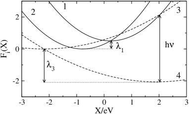
Figure 13: Free energy surfaces in the Marcus-Hush picture when the reorganization energy for charge recombination $\lambda_{3}=\lambda_{4}=2.0$ eV is higher than reorganization energy for charge separation $\lambda_{1}=\lambda_{2}=0.5$ eV due to the coupling of the polarizability change to the macroscopic electric field (eqs 14 and 42).

Imagine a situation in which the photoexcited state is significantly more polarizable than the ground state and the charge-separated state has about the same polarizability as the photoexcited state, $\Delta\alpha_{\text{CS}}\simeq 0$. Then, in weakly polar solvents, $\lambda_{1}\simeq\lambda_{2}$ and both reorganization energies are small because of the low polarity of the medium. For the charge recombination reaction, $\Delta m<0$ and $\Delta\alpha_{\text{CR}}<0$. The permanent dipole $\Delta m$ and the induced dipole $\Delta\alpha F_{m}$ in eq 42 add up when $F_{m}>0$ and subtract when $F_{m}<0$. In the former case, the charge-recombination reorganization energy $\lambda_{3}\simeq\lambda_{4}$ is higher than the charge-separation reorganization energy $\lambda_{1}\simeq\lambda_{2}$. Note that this picture does not contradict to the energy conservation requirement given by eq 1 since the photoexcited state D^∗–A and the ground state D–A are two different electronic states characterized by different polarizabilities.

The normal-region ET can be realized within the Marcus-Hush picture when the reorganization energy is greater than the charge-recombination free energy gap $\lambda_{3}>\Delta F_{\text{CR}}$ (Figure 13). As in Figure 12(a), the energetic efficiency is about 50%, and it drops when charge recombination is shifted into the normal region. However, even in this limit of reduced flexibility of altering the ET parameters, the presence of the macroscopic electric field in the expression for the reorganization energy (eqs 14 and 42) opens the door to manipulations of reorganization parameters through proper design of mutual signs of the polarizability change and the direction of the macroscopic field.

We can conclude that the combination of a highly polarizable donor-acceptor complexe with macroscopic electric field creates a principal possibility for suppressing the recombination reaction in photosynthetic ET. From a more general perspective, the notion of non-equal reorganization energies and non-parabolic free energy surfaces, compliant with the condition of energy conservation (eq 1), opens the door to new models of ET activation which may eventually lead to a practical solution of the photosynthesis problem.

- (1) Marcus, R. A. Rev. Mod. Phys. 1993, 65, 599.
- (2) Wasielewski, M. R. Chem. Rev. 1992, 92, 435.
- (3) Gust, D.; Moore, T. A.; Moore, A. L. Acc. Chem. Res. 1993, 26, 198.
- (4) Bixon, M.; Jortner, J. Adv. Chem. Phys. 1999, 106, 35.
- (5) Kakitani, T.; Mataga, N. J. Phys. Chem. 1985, 89, 8.
- (6) Hwang, J.-K.; Warshel, A. J. Am. Chem. Soc. 1987, 109, 715.
- (7) Tachiya, M. Chem. Phys. Lett. 1989, 159, 505.
- (8) Matyushov, D. V.; Voth, G. A. J. Chem. Phys. 2000, 113, 5413.
- (9) Kuharski, R. A.; Bader, J. S.; Chandler, D.; Sprik, M.; Klein, M. L.; Impey, R. W. J. Chem. Phys. 1988, 89, 3248.
- (10) Marchi, M.; Gehlen, J. N.; Chandler, D.; Newton, M. J. Am. Chem. Soc. 1993, 115, 4178.
- (11) Yelle, R. B.; Ichiye, T. J. Phys. Chem. B 1997, 101, 4127.
- (12) Hartnig, C.; Koper, M. T. M. J. Chem. Phys. 2001, 115, 8540.
- (13) Matyushov, D. V. J. Chem. Phys. 2004, 120, 7532.
- (14) Steffen, M. A.; Lao, K.; Boxer, S. G. Science 1994, 264, 810.
- (15) Middendorf, T. R.; Mazzola, L. T.; Lao, K.; Steffen, M. A.; Boxer, S. G. Biochim. Biophys. Acta 1993, 1143, 223.
- (16) Kjellberg, P.; He, Z.; Pullerits, T. J. Phys. Chem. B 2003, 107, 13737.
- (17) Matyushov, D. V.; Voth, G. A. J. Phys. Chem. A 1999, 103, 10981.
- (18) Small, D. W.; Matyushov, D. V.; Voth, G. A. J. Am. Chem. Soc. 2003, 125, 7470.
- (19) Gupta, S.; Matyushov, D. V. J. Phys. Chem. A 2004, 108, 2087.
- (20) Wei, D.; Patey, G. N. Phys. Rev. Lett. 1992, 68, 2043.
- (21) Zhang, H.; Widom, M. Phys. Rev. B 1995, 51, 8951.
- (22) Morozov, K. I. J. Chem. Phys. 2003, 119, 13024.
- (23) Wei, D.; Patey, G. N.; Perera, A. Phys. Rev. E 1993, 47, 506.
- (24) Bixon, M.; Jortner, J.; Mechel-Beyerle, M. E. Chem. Phys. 1995, 197, 389.
- (25) Allen, M. P.; Tildesley, D. J. Computer Simulation of Liquids; Clarendon Press: Oxford, 1996.
- (26) Weis, J.-J. J. Chem. Phys. 2005, 123, 044503.
- (27) Binder, K.; Heermann, D. W. Monte Carlo Simulation in Statistical Physics; Springer-Verlag: Berlin, 1992.
- (28) Vertogen, G.; Jeu, V. W. H. D. Thermotropic Liquid Cristals, Fundamentals; Springer-Verlag: Berlin, 1988.
- (29) Matyushov, D. V.; Ladanyi, B. M. J. Chem. Phys. 1999, 110, 994.
- (30) Huynh, H. V.; Dattelbaum, D. M.; Meyer, T. J. Coord. Chem. Rev. 2004, 249, 457.
- (31) Alstrum-Acevedo, J. H.; Brennman, M. K.; Meyer, T. J. Inorg. Chem. 2005, 44, 6802.
- (32) Hoertz, P. G.; Mallouk, T. E. Inorg. Chem. 2005, 44, 6828.
- (33) Lewis, N. S. Inorg. Chem. 2005, 44, 6900.