On the number of circuits in random graphs

Abstract

We apply in this article (non rigorous) statistical mechanics methods to the problem of counting long circuits in graphs. The outcomes of this approach have two complementary flavours. On the algorithmic side, we propose an approximate counting procedure, valid in principle for a large class of graphs. On a more theoretical side, we study the typical number of long circuits in random graph ensembles, reproducing rigorously known results and stating new conjectures.

I Introduction

Random graphs Bollo_book ; Janson_book appeared in the mathematical literature as a convenient tool to prove the existence of graphs with a certain property: instead of a direct constructive proof exhibiting such a graph, one can construct a random ensemble of graphs and show that this property is true with a positive probability. Soon afterwards the study of random graphs acquired interest on its own and led to many beautiful mathematical results. A large class of problems in this field can be formulated in the following generic way: a graph $H$ being given, what is the probability that a graph $G$ extracted from the random ensemble under consideration contains $H$ as a subgraph? With a more quantitative ambition, one can define ${\cal N}_{H}(G)$ as the random variable counting the number of occurrences of distinct copies of $H$ in $G$, and study its distribution. These problems are relatively simple when the pattern $H$ remains of a finite size in the thermodynamic limit, i.e. when the size of the random graph $G$ diverges. The situation can become much more involved when $H$ and $G$ have large sizes of the same order, as ${\cal N}_{H}(G)$ can grow exponentially with the system size.

In this article we shall consider these questions when the looked for subgraph $H$ is a long circuit (also called loop or cycle), i.e. a closed self-avoiding path visiting a finite fraction of the vertices of the graph. The level of accuracy of the rigorous results on this problem depends strongly on the random graph ensemble Bollo_book ; Janson_book ; Wormald_review . The regular case (when all vertices of the graph have the same degree $c$) is the best understood one. It has for instance been shown that $c$-regular random graphs with $c\geq 3$ have with high probability Hamiltonian circuits (circuits which visit all vertices of the graph) and the distribution of their numbers is known Robinson_ham ; Janson_ham . This study has been generalized to circuits of all length in Garmo . Less is known for the classical Erdös-Rényi ensembles, where the degree distribution of the vertices converges to a Poisson law of mean $c$. Most results concerns either the neighborhood of the percolation transition at $c=1$ Janson_distrib ; Luczak ; Flaj , or the opposite limit of very large mean connectivity, either finite with respect to the size of the graph Frieze or diverging like its logarithm Posa (it is in this latter regime that the graphs become Hamiltonian). We shall repeatedly come back in the following on this discrepancy between regular random graphs where probabilistic methods have been proved so successful and the other ensembles for which they do not seem powerful enough and might be profitably complemented by approaches inspired by statistical mechanics. We will discuss in particular a conjecture formulated by Wormald Wormald_review , according to which random graph ensembles with a minimal degree of 3 (and bounded maximal degree) should be Hamiltonian with high probability.

Besides this probabilistic point of view (what are the characteristics of the random variable associated to the number of circuits), the problem has also an algorithmic side: how to count the number of circuits in a given graph? Exhaustive enumeration, even using smart algorithms Johnson , is restricted to small graphs as the number of circuits grows exponentially with the size. More formally, the decision problem of knowing if a graph is Hamiltonian (i.e. that it contains a circuit visiting all vertices) is NP-complete GaJo . A probabilistic algorithm for the approximate counting of Hamiltonian cycles is known proba_Hamilton , but is restricted to graphs with large minimal connectivity.

Random graphs have also been largely considered in the physics literature, mainly in the real-world networks perspective AlBa , i.e. in order to compare the characteristics of observed networks, of the Internet for instance, with those of proposed random models. Empirical measures for short loops in real world graphs were for instance presented in BiCaCo . Long circuits visiting a finite fraction of the vertices were also studied in ben . The behavior of cycles in the neighborhood of the percolation transition was considered in BenKra , and the average number of circuits for arbitrary connectivity distribution was computed in BiMa .

In this paper we shall turn the counting problem into a statistical mechanics model, which we treat within the Bethe approximation. This will led us to an approximate counting algorithm, cf. Sec. II. We will then concentrate on random graph ensembles and compute the typical number of circuits with the cavity replica-symmetric method MePa_Bethe in Sec. III. The next two sections will be devoted to the study of the limits of short and longest circuits, then we shall investigate the validity of the replica-symmetry assumption in Sec. VI. We perform a comparison with exhaustive enumerations on small graphs in Sec. VII and draw our conclusions in Sec. VIII. Three appendices collect more technical computations. A short account of our results has been published in EPL .

II A statistical mechanics model and its Bethe approximation

II.1 Derivation of the BP equations

Let us consider a graph $G$ on $N$ vertices (also called sites in the following) $i=1,\dots,N$, with $M$ edges (or links) $l=1,\dots,M$. The notation $l=\langle ij\rangle$ shall mean that the edge $l$ joins the vertices $i$ and $j$. The degree, or connectivity, of a site is the number of links it belongs to. The graphs are assumed in the main part of the text to be simple, i.e. without edges from one vertex to itself or multiple edges between two vertices. We denote $\partial i$ the set of neighbors of the vertex $i$, and use the symbol $\setminus$ to subtract an element of a set: if $j$ is a neighbor of $i$, $\partial i\setminus j$ will be the set of all neighbors of $i$ distinct of $j$. The same symbol $\partial i$ will be used for the set of edges incident to the vertex $i$, the context will always clarify which of the two meanings is understood.

A circuit of length $L$ is an ordered set of $L$ different vertices, $(i_{1},\dots,i_{L})$, such that $\langle i_{n}i_{n+1}\rangle$ is an edge of the graph for all $n\in[1,L-1]$, as well as $\langle i_{L}i_{1}\rangle$. Two circuits are distinct if they do not share the same set of edges (i.e. the starting point and the orientation of a tour along the vertices is not relevant), and we denote ${\cal N}_{L}(G)$ the number of distinct circuits of length $L$ in a graph $G$.

The degrees of freedom of our model are $M$ variables $S_{l}\in\{0,1\}$ placed on the edges of the graph, with their global configuration called $\underline{S}=\{S_{1},\dots,S_{M}\}$. We shall also use $\underline{S}_{i}=\{S_{l}|l\in\partial i\}$ for the configuration of the variables on the links around the vertex $i$. We introduce the following probability law on the space of configurations:

$$p(\underline{S})=\frac{1}{Z(u)}w(\underline{S})\ ,\qquad w(\underline{S})=\left(\prod_{l=1}^{M}\widehat{w}_{l}(S_{l})\right)\left(\prod_{i=1}^{N}w_{i}(\underline{S}_{i})\right)\ ,$$ (1)

where $Z(u)$ is the normalization constant, and the weights $\widehat{w}_{l}$, $w_{i}$ are given by

$$\widehat{w}_{l}(S_{l})=u^{S_{l}}\ ,\qquad w_{i}(\underline{S}_{i})=\begin{cases}1\quad\mbox{if}\quad\underset{l\in\partial i}{\sum}S_{l}\in\{0,2\}\\ 0\quad\mbox{otherwise}\end{cases}\ .$$ (2)

By convention $w_{i}=1$ if $\partial i=\emptyset$, that is to say if the vertex $i$ is isolated. The relevance of this model for the counting of circuits is unveiled by the following reasoning. Each configuration $\underline{S}$ can be associated to a subgraph of $G$, retaining only the edges $l$ such that $S_{l}=1$. The probability (with respect to the law (1)) of such a subgraph is non zero only if the retained edges form closed circuits (any site $i$ is constrained by $w_{i}$ to be surrounded by either 0 or 2 edges of the subgraph), and in that case it is proportional to $u^{L}$ with $L$ the number of its edges. This implies that the normalization factor $Z(u)$ is the generating function of the numbers ${\cal N}_{L}(G)$,

$$Z(u)=\sum_{L}u^{L}{\cal N}_{L}(G)\ .$$ (3)

A precision should be made at this point: we defined above a circuit as a self-avoiding closed path. From the weights on the configurations defined by Eqs. (1,2), ${\cal N}_{L}(G)$ counts in fact the number of configurations made of possibly several vertex disjoint circuits, of total length $L$. In the following we shall concentrate on the limit of large graph and of long circuits, and we expect the leading order behaviour of ${\cal N}_{L}$ not to be affected by this subtlety (see App. A.4 for a combinatorial argument in favour of this thesis), that will be kept understood from now on. Note also that MC_enumeration proposed a Monte Carlo Markov Chain algorithm for the evaluation of such a partition function.

We are thus performing a canonical computation where the length of the circuits is allowed to fluctuate around a mean value fixed by the conjugate external parameter $u$. In the thermodynamic limit $N\to\infty$ the saddle-point method can be used to evaluate the sum (3). Defining $f(u)=\frac{1}{N}\ln Z(u)$ and $\sigma(\ell)=\frac{1}{N}\ln{\cal N}_{L=\ell N}$, where $\ell=L/N$ is a reduced intensive length, one obtains:

$$f(u)=\max_{\ell}[\ell\ln u+\sigma(\ell)]\ .$$ (4)

In this limit the fluctuations of the intensive circuit length in the canonical ensemble vanishes, $\ell$ is concentrated around its mean value $\ell(u)=uf^{\prime}(u)$. The (concave hull of the) microcanonical entropy can thus be obtained from the canonical free-energy (with a slight abuse of terminology we shall use this denomination for $f(u)$) by an inverse Legendre transform,

$$\sigma(\ell)=\min_{u}[f(u)-\ell\ln u]\ .$$ (5)

We shall now use the Bethe approximation to obtain an estimation of the generating function $Z(u)$. We sketch first the general strategy to derive Bethe approximations of statistical models (see Yedidia for a comprehensive discussion), before applying it to the present case.

Consider a (non-negative) weight function $w(\underline{S})$ defined on a space of configurations $\{\underline{S}\}$. The computation of the partition function, $Z=\sum_{\underline{S}}w(\underline{S})$, can be reformulated as an extremization problem. Indeed, the Gibbs functional free-energy,

$$F_{\rm Gibbs}[p_{\rm v}]=\sum_{\underline{S}}p_{\rm v}(\underline{S})\ln\left(\frac{p_{\rm v}(\underline{S})}{w(\underline{S})}\right)\ ,$$ (6)

is minimal (in the space of normalized variational distributions) for $p_{\rm v}(\underline{S})=p(\underline{S})=w(\underline{S})/Z$, where it takes the value $(-\ln Z)$. In general finding the minimum of this functional is not simpler than a direct computation of $Z$, however this formulation opens the way to variational approaches: the minimum of $F_{\rm Gibbs}$ in a restricted set of trial distributions $p_{\rm v}$, more easily parametrized than generic ones, yields an upper bound on $(-\ln Z)$. The simplest implementation of this idea is the mean-field approximation, in which the trial distributions are factorized, $p_{\rm v}(\underline{S})=\prod_{l}p_{l}(S_{l})$. A natural refinement consists in introducing correlations between neighboring variables in the trial distributions. Consider for instance a weight function of the form (1), for arbitrary $\widehat{w}_{l}$ and $w_{i}$. One can easily show that if the underlying graph $G$ were a tree, the true probability distribution would be given by

$$p(\underline{S})=\left(\prod_{l=1}^{M}p_{l}(S_{l})\right)^{-1}\left(\prod_{i=1}^{N}p_{i}(\underline{S}_{i})\right)\ ,$$ (7)

where $p_{l}$ and $p_{i}$ are the exact marginals (for instance, $p_{l}(S_{l})=\sum_{\underline{S}\setminus S_{l}}p(\underline{S})$) of the law $p$. When the graph is not a tree, this expression is not valid any more. The Bethe approximation consists however in assuming that trial probability distributions can be approximately written under this form even if the graph contains cycles. This yields the so-called Bethe free-energy,

$$F_{\rm Bethe}[\{p_{i}\},\{p_{l}\}]=\sum_{i=1}^{N}\sum_{\underline{S}_{i}}p_{i}(\underline{S}_{i})\ln\left(\frac{p_{i}(\underline{S}_{i})}{w_{i}(\underline{S}_{i})}\right)-\sum_{l=1}^{M}\sum_{S_{l}}p_{l}(S_{l})\ln\left(p_{l}(S_{l})\widehat{w}_{l}(S_{l})\right)\ .$$ (8)

This free-energy is to be minimized with respects to the approximate marginals $p_{l}$, $p_{i}$, which have to respect two types of constraints:

• $p_{l}$ and $p_{i}$ are normalized.

• they are consistent, i.e. for each link $l=\langle ij\rangle$, one has

  $$p_{l}(S_{l})=\sum_{\underline{S}_{i}\setminus S_{l}}p_{i}(\underline{S}_{i})=\sum_{\underline{S}_{j}\setminus S_{l}}p_{j}(\underline{S}_{j})\ .$$ (9)

This constrained minimization can be performed considering the $\{p_{i}\},\{p_{l}\}$ as independent, at the price of the introduction of Lagrange multipliers to enforce the conditions (9). It is well known that such a procedure amounts to look for a fixed point of the corresponding belief propagation (BP) equations Yedidia . In this setting the Lagrange multipliers are interpreted as messages sent by variables to neighboring constraints, and vice-versa.

Let us now apply this formalism to the specific weights defined in Eq. (2). A peculiarity of $w_{i}$ has to be kept in mind: it can be strictly vanishing when the geometrical constraint of having 0 or 2 present edges around each vertex is not fulfilled. As a consequence, the approximate variational marginals $p_{i}(\underline{S}_{i})$ have to respect this constraint, and vanish when $w_{i}(\underline{S}_{i})=0$. The Bethe free-energy reads now

$$F_{\rm Bethe}[\{p_{i}\},\{p_{l}\}]=\sum_{i=1}^{N}\sum_{\underline{S}_{i}}p_{i}(\underline{S}_{i})\ln\left(p_{i}(\underline{S}_{i})\right)-\sum_{l=1}^{M}\sum_{S_{l}}p_{l}(S_{l})\ln\left(p_{l}(S_{l})u^{S_{l}}\right)\ ,$$ (10)

where the convention $0\ln 0=0$ has been used, for the strictly forbidden configurations with $w_{i}(\underline{S}_{i})=0$ not to contribute to $F_{\rm Bethe}$.

A possible parametrization of the marginals achieving the extremum of the Bethe free-energy is

$$p_{l}(S_{l})=\frac{1}{C_{l}}(u\,y_{i\to j}\,y_{j\to i})^{S_{l}}\ ,\qquad p_{i}(\underline{S}_{i})=\frac{1}{C_{i}}w_{i}(\underline{S}_{i})\prod_{j\in\partial i}(u\,y_{j\to i})^{S_{\langle ij\rangle}}\ ,$$ (11)

where the $C_{l}$ and $C_{i}$ are normalization constants, and for each link $\langle ij\rangle$ of the graph a pair of directed (real positive) messages has been introduced, $y_{i\to j}$ and $y_{j\to i}$. These messages obey the following BP equations,

$$y_{i\to j}=\frac{u\underset{k\in\partial i\setminus j}{\sum}y_{k\to i}}{1+\frac{1}{2}u^{2}\underset{\underset{k\neq k^{\prime}}{k,k^{\prime}\in\partial i\setminus j}}{\sum}y_{k\to i}\ y_{k^{\prime}\to i}}\ ,$$ (12)

cf. Fig. 1 for a graphical representation. Roughly speaking, $y_{i\to j}$ is proportional to the probability that the edge $\langle ij\rangle$ would be present if the constraint $w_{j}$ and the weight $u^{S_{l}}$ were to be discarded. Hence the form of Eq. (12): the numerator corresponds to the situation where $\langle ij\rangle$ is present, the constraint $w_{i}$ imposes then that exactly one of the edges of $\partial i\setminus j$ is also present. The denominator states on the contrary that if $\langle ij\rangle$ is absent, either none or two of the edges of $\partial i\setminus j$ are present.

Figure 1: The messages involved in Eq. (12).

The normalization constants of the marginals are easily computed,

$$C_{l}=1+u\,y_{i\to j}\,y_{j\to i}\ ,\qquad C_{i}=1+\frac{1}{2}u^{2}\underset{\underset{k\neq k^{\prime}}{k,k^{\prime}\in\partial i}}{\sum}y_{k\to i}\ y_{k^{\prime}\to i}\ ,$$ (13)

and one can check, using the BP equations, that the consistency conditions are indeed respected by these expressions of the marginals. Moreover the value of $F_{\rm Bethe}$ at its minimum can be expressed in terms of the normalization constants $C_{i}$ and $C_{l}$. Using this value as an approximation for $-\ln Z(u)$ the free energy in the Bethe approximation can be written as:

$$Nf(u)=-\sum_{l=1}^{M}\ln(C_{l})+\sum_{i=1}^{N}\ln(C_{i})\ .$$ (14)

One should also compute the length of the circuits in the configurations selected at a given value of $u$, $\ell(u)=uf^{\prime}(u)$. It is rather unwise to use Eq. (14) to compute the derivative $f^{\prime}(u)$, as this expression involves the messages which are solution of the BP equations and hence have a non trivial dependence on $u$. On the contrary the expression (10) being variational, it is enough to compute its explicit derivative with respects to $u$ to obtain:

$$\ell(u)=\frac{1}{N}\sum_{l=1}^{M}p_{l}(1)=\frac{1}{N}\sum_{\langle ij\rangle}\frac{u\,y_{i\to j}\,y_{j\to i}}{1+u\,y_{i\to j}\,y_{j\to i}}\ .$$ (15)

The first equality is natural, the average length of the circuits being equal to the sum of the probabilities of presence of all the edges of the graph. Note also that the marginal probabilities contain individually some local information: for instance $p_{l}(1)$ is the fraction of circuits of length $\ell(u)$ which go through the particular link $l$.

Let us now come back for an instant on the BP equations and underline two simple properties they possess. In Eq. (12) we used the natural convention that sums on empty sets are null. The first consequence is that $y_{i\to j}=0$ if $j$ is the only neighbor of $i$, as $\partial i\setminus j=\emptyset$. In such a situation $i$ is indeed a leaf of the graph, and no circuits can go through the edge $\langle ij\rangle$. Even if in general the directed message in the reverse direction $y_{j\to i}$ is non zero, one can easily check that the edge $\langle ij\rangle$ does not contribute to the free energy. In other words the physical observables are unaffected by the leaf removal process, in which the graph $G$ is deprived of the dangling edge $\langle ij\rangle$. Moreover this simplification can be iteratively repeated, until no leaves are present in the remaining graph. An illustration of this process in terms of the null directed messages is given in the left part of Fig. 2. This property of the BP equations reflects the fact that the circuits of a graph are necessarily part of its 2-core, that is to say the largest of its subgraphs in which all sites have connectivity at least 2.

Consider now a site $i$ with two neighbors $j$ and $k$, for which the BP equations read $y_{i\to j}=uy_{k\to i}$ and $y_{i\to k}=uy_{j\to i}$. This implies that along a chain of degree 2 sites, the directed messages follow a geometric progression, cf. the right part of Fig. 2, and in consequence one easily shows that the marginal probability of all edges in a chain are equal: if a circuit goes through one of the edges of the chain, it must go through all of it.

Figure 2: Left: the leaf removal procedure interpreted in terms of null messages. Right: the behaviour of messages along chains of degree 2 vertices.

II.2 An approximate counting algorithm

The presentation of the Bethe approximation in terms of messages Yedidia we followed in the previous section suggests in a very natural way the following algorithm for the approximate counting of long circuits in a given graph:

• initialize messages $y_{i\to j}$ for each directed edge of the graph to some random positive values.

• iterate the BP equations (12) at a given value of $u$ until convergence has been reached.

• using the messages solution of the BP equations, compute $f(u),\ell(u)$ from Eqs. (14,15), and $\sigma(\ell(u))=f(u)-\ell(u)\ln u$ (cf. Eq. (5)).

• repeat this procedure for different values of $u$ to obtain a plot of $\sigma(\ell)$ parametrized by $u$.

This algorithm is of course far from being exact. A first limitation is that the BP equations are not a priori convergent, on the contrary it is easy to construct counter-examples of small graphs on which they do not reach any fixed point. It would thus be interesting to determine under which conditions the convergence towards an unique (non-trivial) fixed point is ensured. This kind of question has been the subject of recent interest, see for instance Tati ; Heskes . Another possible criticism is that even in the case of convergence of the BP equations, the prediction for the number of loops relies on the Bethe approximation, which is an uncontrolled one. This being said, one should however keep in mind that for large graphs with numerous circuits, an exact enumeration Johnson is computationally very expensive and reaches very soon the limitations of present time computers. The approximate algorithm we introduced here can then serve as an efficient alternative, even if its predictions should be treated with caution.

We presented in EPL the results of such a procedure when applied to a real-world network of the Autonomous System Level description of the Internet DIMES , allowing to estimate the total number of circuits, the length of the most numerous circuits and the maximal length circuits, obtaining numbers which are far beyond the possibilities of exhaustive counting. We also checked the compatibility of our results with the direct enumeration of very short circuits.

III The typical number of circuits in random graphs ensembles

III.1 Definitions

The rest of the paper shall be devoted to the study of the number of circuits in graphs $G$ belonging to random ensembles. In the regime we are interested in (long circuits of large graphs with finite mean degree), the common wisdom about the statistical mechanics of disordered systems is that the random variable $\log({\cal N}_{L=N\ell})/N$ should be concentrated around its average, the quenched entropy $\sigma_{\rm q}(\ell)$. More formally, one expects the existence of a constant $\ell_{\rm max}\in[0,1]$ and a function $\sigma_{\rm q}(\ell)>0$ defined on $]0,\ell_{\rm max}]$ such that for any sequence $L_{N}$ with $L_{N}/N\to\ell$,

$${\rm if}\ \ell>\ell_{\rm max}\ , {\rm Prob}[{\cal N}_{L_{N}}>0]\to 0\ ,$$ (16)

$${\rm if}\ \ell\in]0,\ell_{\rm max}]\ , \forall\epsilon>0\ \ \ {\rm Prob}\left[\left|\frac{1}{N}\log{\cal N}_{L_{N}}-\sigma_{\rm q}(\ell)\right|\geq\epsilon\right]\to 0\ .$$ (17)

In the second line $\log(0)$ should be interpreted as $-\infty$, i.e. outside of any finite interval.

The standard probabilistic methods for proving this kind of results rely essentially on the combinatorial computation of the average and variance of ${\cal N}_{L}$, which are then used in the Markov and Chebyshev inequalities (first and second method). The rigorous results on the number of circuits in regular random graphs Wormald_review ; Robinson_ham ; Janson_ham ; Garmo have indeed be obtained through a refined version of the second moment method (see theorem 4.1 in Wormald_review ). In this context this approach is limited to cases where the second moment of ${\cal N}_{L}$ is not exponentially larger than the square of its first moment. The quenched entropy is then shown to be equal to the annealed one, $\sigma_{\rm a}(\ell)=\lim\log(\overline{{\cal N}_{\ell N}})/N$, where the overline denotes the average over the random graph ensemble.

We believe that in all ensembles of graphs which are not strictly regular and have a fastly decaying connectivity distribution, the second moment of the number of long circuits is exponentially larger that the square of the first moment (details of the combinatorial computations leading to this belief are presented in App. A), thus ruling out the main probabilistic techniques used so far. The annealed entropy BiMa is in this case strictly larger than the quenched one, as it is dominated by exponentially rare graphs which have exponentially more circuits than the typical ones.

We shall now follow the cavity method MePa_Bethe , which is particularly well suited to tackle this problem, ubiquitous in the field of disordered statistical mechanics models Beyond . According to this view, the quenched entropy controlling the leading behaviour of the number of circuits in the typical graphs depends on the graph ensemble only through its limiting degree distribution $q_{k}$ . We can for instance assume that the graphs are drawn uniformly among all graphs on $N$ vertices which have this degree distribution. Let us recall the existence in this case of a percolation transition MR ; NeStWa between a low connectivity regime where the connected components of the graph are essentially trees of finite size, to a percolated phase where one giant component contains a finite fraction of the vertices.

Before proceeding with the computations, we introduce some notations used in the following. $c=\sum_{k}kq_{k}$ denotes the mean connectivity of the graph, hence the number of edges is in the thermodynamic limit $M=Nc/2$. $\tilde{q}_{k}$ will be the offspring probability, that is to say the probability of finding a site of degree $k+1$ when selecting at random an edge of the graph and then one of its two vertices. As a site is encountered in such a selection with a probability proportional to its degree, $\tilde{q}_{k}$ is proportional to $(k+1)q_{k+1}$. By normalization,

$$\tilde{q}_{k}=\frac{(k+1)q_{k+1}}{c}\ .$$ (18)

To simplify notations we shall also define the factorial moments of $q_{k}$ and $\tilde{q}_{k}$ as

$$\mu_{n}=\sum_{k=n}^{\infty}q_{k}\,k(k-1)\dots(k-n+1)\ ,\quad\tilde{\mu}_{n}=\sum_{k=n}^{\infty}\tilde{q}_{k}\,k(k-1)\dots(k-n+1)\ ,\quad\mu_{n}=c\tilde{\mu}_{n-1}\ ,$$ (19)

where the last relation is a simple consequence of Eq. (18).

The condition for percolation MR ; NeStWa reads with these notations $\tilde{\mu}_{1}>1$. We shall assume in the following that this condition is met: the long circuits we are studying cannot be present if the graph has no giant component.

We restrict ourselves to fastly (i.e. faster than any power law) decaying distributions of connectivities, such that all their moments are finite. After stating the results for arbitrary $q_{k}$ we shall often specialize to Poissonian graphs of mean connectivity $c$, i.e. such that $q_{k}=e^{-c}c^{k}/k!$.

III.2 The quenched computation

In essence the computation of the quenched entropy we undertake now amounts to perform the Bethe approximation of the statistical model defined by Eqs. (1,2) for graphs generated according to the connectivity distribution $q_{k}$. The solution of the BP equations (12), which depends on the particular graph on which they are applied, leads then to a random set of messages $y$. Taking at random a graph of the ensemble, and a directed edge of this graph, one finds a message $y$ with probability distribution $P(y;u)$. In the so-called cavity method at the replica-symmetric level MePa_Bethe , one assumes that the incoming messages on this directed edge are independent random variables with the same probability law $P(y;u)$. Using Eq. (12), this is turned into a self-consistent equation,

$$P(y;u)=\tilde{q}_{0}\,\delta(y)+\sum_{k=1}^{\infty}\tilde{q}_{k}\int_{0}^{\infty}dy_{1}\,P(y_{1};u)\dots dy_{k}\,P(y_{k};u)\,\delta(y-g_{k}(y_{1},\dots,y_{k}))\ ,$$ (20)

where we have defined

$$g_{1}(y_{1})=uy_{1}\ ,\qquad g_{k}(y_{1},\dots,y_{k})=\frac{u\overset{k}{\underset{i=1}{\sum}}y_{i}}{1+u^{2}\underset{1\leq i<j\leq k}{\sum}y_{i}y_{j}}\ {\rm for}\ k\geq 2\ .$$ (21)

The quenched free-energy is then expressed in terms of this $P(y;u)$ as (cf. Eq. (14)):

$$f_{\rm q}(u) = \sum_{k=2}^{\infty}q_{k}\int_{0}^{\infty}dy_{1}\,P(y_{1};u)\dots dy_{k}\,P(y_{k};u)\,\ln\left(1+u^{2}\sum_{1\leq i<j\leq k}y_{i}y_{j}\right)$$ (22)

$$-\frac{c}{2}\int_{0}^{\infty}dy_{1}\,P(y_{1};u)\,dy_{2}\,P(y_{2};u)\,\ln(1+u\,y_{1}y_{2})\ ,$$

In a similar way the length of the circuits in the configurations selected by a given value of $u$, and the corresponding quenched entropy read:

$$\ell(u) = \frac{c}{2}\int_{0}^{\infty}dy_{1}\,P(y_{1};u)\,dy_{2}\,P(y_{2};u)\,\frac{uy_{1}y_{2}}{1+uy_{1}y_{2}}\ ,$$ (23)

$$\sigma_{\rm q}(\ell(u)) = f_{\rm q}(u)-\ell(u)\ln u\ .$$ (24)

As appears clearly when considering Eq. (20), the distribution $P(y;u)$ contains a Dirac’s delta in $y=0$, that is to say a finite fraction of the messages are strictly vanishing. Let us call $\eta$ the fraction of non-trivial messages, and $\widehat{P}(y;u)$ their (normalized) distribution, i.e. $P(y;u)=(1-\eta)\,\delta(y)+\eta\,\widehat{P}(y;u)$ where $\widehat{P}$ does not contain a Dirac’s delta in $y=0$. Inserting this definition in Eq. (20), one obtains the equation satisfied by $\eta$,

$$1-\eta=\sum_{k=0}^{\infty}\tilde{q}_{k}(1-\eta)^{k}\ .$$ (25)

Besides the trivial solution $\eta=0$, this equation has another positive solution as soon as $\tilde{\mu}_{1}>1$, i.e. when the graph is in the percolating regime. One also realizes that $\widehat{P}$ satisfies the equation obtained from Eq. (20) by replacing the offspring distribution $\tilde{q}$ by $\tilde{r}$, defined as

$$\tilde{r}_{0}=0\ ,\qquad\tilde{r}_{k}=\sum_{n=k}^{\infty}\tilde{q}_{n}{n\choose k}\eta^{k-1}(1-\eta)^{n-k}\quad{\rm for}\ k\geq 1\ .$$ (26)

Finally the free-energy and the typical length of circuits (cf. Eqs. (22,23)) can also be expressed in terms of the simplified distribution $\widehat{P}$, if one replaces $q$ by the following distribution $r$:

$$r_{0}=1-\sum_{k\geq 2}r_{k}\ ,\quad r_{1}=0\ ,\quad r_{k}=\sum_{n=k}^{\infty}q_{n}{n\choose k}\eta^{k}(1-\eta)^{n-k}\quad{\rm for}\ k\geq 2\ .$$ (27)

It is easily verified that this modified distribution has mean $c\eta^{2}$, and that a relation similar to Eq. (18) holds between $r$ and $\tilde{r}$,

$$\tilde{r}_{k}=\frac{(k+1)r_{k+1}}{c\eta^{2}}\ .$$ (28)

Let us now give the interpretation of this simplification process. We have shown the equality of the quenched entropy of the circuits in the two ensembles defined one by $q_{k}$, the other by $r_{k}$. As we explained at the end of Sec. II, the circuits of a graph $G$ necessarily belong to its 2-core, that is to say the largest subgraph of $G$ in which all vertices have a degree at least equal to two. On the dangling ends, i.e. the edges that do not belong to the 2-core, at least one of the two directed messages $y$ is equal to zero. It is thus very natural to interpret the elimination of null messages in terms of the typical properties of the 2-core of graphs drawn from the ensemble defined by the distribution $q_{k}$. The fraction of edges in the 2-core should be $\eta^{2}$, as both directed messages have to be non-zero for the edge to belong to the 2-core, $r_{k}$ (resp. $\tilde{r}_{k}$) should be the connectivity (resp. offspring) distribution of the 2-core. This interpretation is indeed confirmed by a direct study of a leaf-removal algorithm which iteratively removes the dangling ends of a graph, that we present in App. B. In the following we shall use the distribution $q$ or $r$, depending on which is simpler in the encountered context.

For future use we give the explicit expressions in the case of Poissonian random graphs,

$$\eta=1-e^{-c\eta}\ ,\qquad r_{k}=\frac{e^{-c\eta}(c\eta)^{k}}{k!}\ \ \ {\rm for}\ \ k\geq 2\ ,\qquad\tilde{r}_{k}=\frac{1}{\eta}\frac{e^{-c\eta}(c\eta)^{k}}{k!}\ \ \ {\rm for}\ \ k\geq 1\ .$$ (29)

We now come back to the predictions of the quenched entropy and consider as a first example the case of regular graphs of connectivity $c$, for which $\tilde{q}_{k}=\delta_{k,c-1}$. Equation (20) on the distribution of messages has then a very simple solution, $P(y;u)=\delta(y-y_{\rm r}(u,c))$, with

$$y_{\rm r}(u,c)=\sqrt{\frac{2u(c-1)-2}{u^{2}(c-1)(c-2)}}\ .$$ (30)

It is then straightforward to express $\ell(u)$ and $\sigma_{\rm q}(\ell(u))$ from this solution. One can also eliminate the parametrization by $u$ to obtain the entropy,

$$\sigma_{\rm r}(\ell,c)=-(1-\ell)\ln(1-\ell)+\left(\frac{c}{2}-\ell\right)\ln\left(1-\frac{2\ell}{c}\right)+\ell\ln(c-1)\ ,$$ (31)

which corresponds to the known results mentioned above Garmo ; MaMo .

The peculiarity of the regular case for which annealed and quenched averages coincide is hinted to by the simplicity of this solution $P(y;u)$ with a single Dirac peak. As soon as $\tilde{q}_{k}$ is positive for more than one connectivity, the distribution $P(y;u)$ acquires a non vanishing support, which we expect to show up as larger fluctuations in the numbers of circuits, and hence a difference between quenched and annealed computations.

The equation on $P(y;u)$ is not solvable analytically for an arbitrary connectivity distribution. Two complementary roads can then be followed: this distributional equation can be easily solved with a population dynamics algorithm MePa_Bethe . One represents $P(y;u)$ by a sample of a large number of $y$’s, at each time step one draws a number $k$ following the law $\tilde{r}_{k}$, extracts $k$ values $y_{1},\dots,y_{k}$ randomly from the population, computes the new value $g_{k}(y_{1},\dots,y_{k})$, and replace one of the representant of the population by this new value. Starting from a random sample of messages, the population converges to a sample of message distributed according to the fixed point solution of Eq. (20). The corresponding physical observables are then computed from this sample of messages, which yields the prediction for $\sigma_{\rm q}(\ell)$. As an illustration, we present in Fig. 3 the results of such a numerical computation for Poissonian graphs of mean degree $c=3$.

On the analytical side, we present in the next sections a study of two limits, for the short and longest circuits, in which the analytical predictions can be pushed forward.

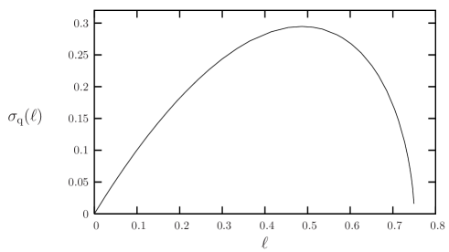
Figure 3: Quenched entropy for a Poissonian graph of mean connectivity 3.

IV The limit of small circuits

We shall investigate in this section the behaviour of the quenched entropy in the limit of small circuits, computing analytically its first two derivatives at the origin, $\sigma_{\rm q}^{\prime}(0)$ and $\sigma_{\rm q}^{\prime\prime}(0)$.

Let us first show the existence of a critical value $u_{\rm m}$ below which the typical configurations are deprived of any circuit. This transition is signaled by an instability of the trivial solution of Eq. (20), $P(y)=\delta(y)$. Perturbing this distribution infinitesimally, one can expand $g_{k}$ as $g_{k}(y_{1},\dots,y_{k})=u\sum_{i=1}^{k}y_{i}+O(y_{i}^{3})$. In this limit, if one inserts in the r.h.s. of Eq. (20) some $P(y)$ with an infinitesimal mean $P_{1}$, one obtains another distribution with a mean $(u/u_{\rm m})P_{1}$, with

$$u_{\rm m}^{-1}=\sum_{k=1}^{\infty}k\tilde{q}_{k}=\tilde{\mu}_{1}\ .$$ (32)

If $u<u_{\rm m}$, the mean of the perturbed distributions decrease upon iteration, so $P(y)=\delta(y)$ is a stable solution. On the contrary if $u>u_{\rm m}$ this solution is unstable and must flow to a non-trivial stable fixed point.

We shall now set up an expansion around the stability limit, $u=u_{\rm m}+\epsilon$ with $\epsilon\to 0^{+}$. In this limit the messages $y$ are supported on a scale which vanishes with $\epsilon$, we shall consequently define $y=x\,\epsilon^{a}+o(\epsilon^{a})$ with $x$ finite, and $a$ a positive exponent to be determined in a few lines. Let us denote $Q(x)$ the distribution of the rescaled messages and relate the moments of $P$ and $Q$ as

$$P_{n}(\epsilon)=\int_{0}^{\infty}dy\,y^{n}P(y;u_{\rm m}+\epsilon)\sim\epsilon^{na}\int_{0}^{\infty}dx\,x^{n}Q(x)=\epsilon^{na}Q_{n}\ .$$ (33)

Expanding Eq. (21) as

$$x\sim u_{\rm m}\sum_{i=1}^{k}x_{i}+\epsilon\sum_{i=1}^{k}x_{i}-u_{\rm m}^{2}\epsilon^{2a}\left(\sum_{i=1}^{k}x_{i}\right)\left(\sum_{1\leq i<j\leq k}x_{i}x_{j}\right)\ ,$$ (34)

we obtain at the lowest order

$$\epsilon = u_{\rm m}^{4}\tilde{\mu}_{2}Q_{2}\epsilon^{2a}+\frac{1}{2}u_{\rm m}^{4}\tilde{\mu}_{3}Q_{1}^{2}\epsilon^{2a}\ ,$$ (35)

$$Q_{2}\epsilon^{2a} = u_{\rm m}Q_{2}\epsilon^{2a}+u_{\rm m}^{2}\tilde{\mu}_{2}Q_{1}^{2}\epsilon^{2a}\ .$$ (36)

This fixes the scale $a=1/2$ and the values of $Q_{1}$ and $Q_{2}$, the first two moments of the distribution solution of

$$Q(x)=\tilde{q}_{0}\,\delta(x)+\sum_{k=1}^{\infty}\tilde{q}_{k}\int_{0}^{\infty}dx_{1}Q(x_{1})\dots dx_{k}Q(x_{k})\,\delta\left(x-u_{\rm m}\sum_{i=1}^{k}x_{i}\right)\ .$$ (37)

Let us now consider the consequences of this scaling on the observables $f_{\rm q}$, $\ell$, $\sigma_{\rm q}$ in the limit $u\to u_{\rm m}$. Taking into account both their explicit dependence on $u$ and the implicit one through the distribution $P(y;u)$, one finds after a short computation that:

• the expansion of $f_{\rm q}(u_{\rm m}+\epsilon)$ starts at the second order,

  $$f_{\rm q}(u_{\rm m}+\epsilon) = f_{\rm q}^{(2)}\epsilon^{2}+O(\epsilon^{3})\ ,$$ (38)

  $$f_{\rm q}^{(2)} = \frac{c}{2}Q_{1}^{2}+\frac{c}{4}u_{\rm m}^{2}(1-u_{\rm m})Q_{2}^{2}-\frac{1}{2}u_{\rm m}^{4}\mu_{3}Q_{1}^{2}Q_{2}-\frac{1}{8}u_{\rm m}^{4}\mu_{4}Q_{1}^{4}\ .$$ (39)

• the intensive length $\ell$ is, at its first non-trivial order,

  $$\ell(u_{\rm m}+\epsilon)=\ell^{(1)}\epsilon+O(\epsilon^{2})\ ,\qquad\ell^{(1)}=\frac{c}{2}u_{\rm m}Q_{1}^{2}\ .$$ (40)

• the first two derivatives of $\sigma_{\rm q}(\ell)$ in $\ell=0$ can be obtained from the previous expressions:

  $$\sigma_{\rm q}^{\prime}(0)=-\ln u_{\rm m}\ ,\qquad\sigma_{\rm q}^{\prime\prime}(0)=\frac{2f_{\rm q}^{(2)}}{(\ell^{(1)})^{2}}-\frac{2}{u_{\rm m}\ell^{(1)}}$$ (41)

Solving for $Q_{1,2}$ and plugging their values in the expression (41) of the derivatives of the entropy one finally obtains:

$$\sigma_{\rm q}^{\prime}(0)=\ln\tilde{\mu}_{1}\ ,\qquad\sigma_{\rm q}^{\prime\prime}(0)=-\frac{1}{c}\left(\frac{\tilde{\mu}_{3}}{\tilde{\mu}_{1}^{2}}+\frac{2\tilde{\mu}_{2}^{2}}{\tilde{\mu}_{1}^{3}(\tilde{\mu}_{1}-1)}\ .\right)$$ (42)

We can now turn to the discussion of these results, and in particular to the comparison with the annealed computation of Bianconi and Marsili BiMa . Expanding their result (reproduced in Eq. (90)) in powers of $\ell$, one obtains

$$\sigma_{\rm a}^{\prime}(0)=\ln\tilde{\mu}_{1}\ ,\qquad\sigma_{\rm a}^{\prime\prime}(0)=-\frac{1}{c}\frac{\tilde{\mu}_{3}+4\tilde{\mu}_{2}-2\tilde{\mu}_{1}(\tilde{\mu}_{1}-1)}{\tilde{\mu}_{1}^{2}}\ .$$ (43)

Let us first consider a large but non extensive circuit length, $1\ll L\ll\ln N$. The number ${\cal N}_{L}$ of such circuits is, in the thermodynamic limit, a Poisson distributed random variable with a mean equal to

$$\frac{1}{2L}\left(\frac{\sum_{k}k(k-1)q_{k}}{\sum_{k}kq_{k}}\right)^{L}=\frac{1}{2L}(\tilde{\mu}_{1})^{L}\ .$$ (44)

When $L\gg 1$ the most probable value of this random variable is equal to its mean, in which one can neglect the polynomial prefactor $1/(2L)$ (we recall that we assume $\tilde{\mu}_{1}>1$ to be in the percolated regime). Consequently the quenched and annealed computation of the first derivative of the entropy at $\ell=0$ coincide and match the result for $1\ll L\ll\ln N$:

$${\cal N}_{L}\sim e^{N\sigma(L/N)}\sim e^{L\sigma^{\prime}(0)}=(\tilde{\mu}_{1})^{L}\ .$$ (45)

On the contrary the second derivatives differ, in general, in the two computations:

$$\sigma_{\rm a}^{\prime\prime}(0)-\sigma_{\rm q}^{\prime\prime}(0)=\frac{2}{c\tilde{\mu}_{1}^{3}(\tilde{\mu}_{1}-1)}(\tilde{\mu}_{2}-\tilde{\mu}_{1}(\tilde{\mu}_{1}-1))^{2}\ .$$ (46)

As expected the annealed entropy is always greater than the quenched one at this order of the expansion. Moreover it is straightforward to show from the above expression that $\sigma_{\rm a}^{\prime\prime}(0)-\sigma_{\rm q}^{\prime\prime}(0)$ vanishes only if the distribution $\tilde{q}_{k}$ is supported by a single integer, in other words in the random regular graph case.

We performed this computation using the degree distribution $q_{k}$ of the graph, however the reader will easily verify that Eq. (42) remains unchanged if one replaces $q_{k}$ by the connectivity distribution $r_{k}$ of its 2-core (the factorial moments $\tilde{\mu}_{n}$ gets multiplied by $\eta^{n-1}$, the mean connectivity $c$ by $\eta^{2}$).

For completeness we state here the results for Poissonian graphs of average degree $c$,

$$\sigma_{\rm q}^{\prime}(0)=\ln c\ ,\quad\sigma_{\rm q}^{\prime\prime}(0)=-\frac{c+1}{c-1}\ .$$ (47)

V The limit of longest circuits

A more interesting limit case is the one of maximal length circuits. Some questions arise naturally in this context: what is the maximal length, $\ell_{\rm max}$, for which circuits of $N\ell_{\rm max}$ edges are present with high probability in a given random graph ensemble? In particular, under which conditions these graphs are Hamiltonian, that is to say $\ell_{\rm max}=1$? Finally, what is the number of such longest circuits, measured by the corresponding quenched entropy $\sigma_{\rm q}(\ell_{\rm max})$? From the properties of the Legendre transform (cf. Eq. (4)), these quantities can be determined by investigating the limit $u\to\infty$ of the free-energy :

$$f_{\rm q}(u)\underset{u\to\infty}{\sim}\ell_{\rm max}\ln u+\sigma_{\rm q}(\ell_{\rm max})\ .$$ (48)

This corresponds, in the jargon of the statistical mechanics approach to combinatorial optimization problems, to a zero temperature limit, where $-\ell_{\rm max}$ (resp. $\sigma_{\rm q}(\ell_{\rm max})$) is the ground-state energy (resp. entropy) density.

It turns out that the answers to the above questions crucially depend on the presence or not of degree 2 sites in the 2-core of the random graphs under study, we shall thus divide the rest of this section according to this distinction. Before that we state an equivalent expression of the free-energy which will prove more convenient in this limit,

$$f_{\rm q}(u)=\sum_{k=3}^{\infty}q_{k}\left(\frac{k}{2}I_{k-1}(u)-\frac{k-2}{2}I_{k}(u)\right)\ ,$$ (49)

where we have defined some logarithmic moments of the distribution $P$,

$$I_{k}(u)=\int_{0}^{\infty}dy_{1}\,P(y_{1};u)\dots dy_{k}\,P(y_{k};u)\ln\left(1+u^{2}\underset{1\leq i<j\leq k}{\sum}y_{i}y_{j}\right)\quad{\rm for}\ k\geq 2.$$ (50)

This form of $f_{\rm q}(u)$ is obtained from Eq. (22) by using the equation (20) on $P(y;u)$ and the identity

$$1+u\,y_{0}\,g_{k}(y_{1},\dots,y_{k})=\frac{1+u^{2}\underset{0\leq i<j\leq k}{\sum}y_{i}y_{j}}{1+u^{2}\underset{1\leq i<j\leq k}{\sum}y_{i}y_{j}}\ .$$ (51)

V.1 In the absence of degree 2 sites in the 2-core

One can gain some intuition on the limit $u\to\infty$ by inspecting the behaviour of the messages in the regular case. Indeed, the expansion of Eq. (30) shows a scaling of the form $y\sim xu^{-1/2}$, with $x$ (an evanescent field in the jargon of optimization problems) finite. Consider now the more general case of random graph ensembles with a minimal connectivity of 3, i.e. $q_{0}=q_{1}=q_{2}=0$, which consequently implies $\tilde{q}_{0}=\tilde{q}_{1}=0$. Thanks to the vanishing of $\tilde{q}_{1}$, the equations (20,21) have a solution with the above scaling of $y$ with $u$. One can also check numerically in particular cases that the distributions $P(y)$ concentrate according to this behaviour for large but finite values of $u$.

Denoting $V_{0}(x)$ the distribution of the evanescent fields, one easily obtains the integral equation it obeys:

$$V_{0}(x)=\sum_{k=2}^{\infty}\tilde{q}_{k}\int_{0}^{\infty}dx_{1}\,V_{0}(x_{1})\dots dx_{k}\,V_{0}(x_{k})\,\delta(x-h_{k}(x_{1},\dots,x_{k}))\ ,\quad{\rm with}\ \ h_{k}(x_{1},\dots,x_{k})=\frac{\overset{k}{\underset{i=1}{\sum}}x_{i}}{\underset{1\leq i<j\leq k}{\sum}x_{i}x_{j}}\ .$$ (52)

Moreover the logarithmic moments defined in Eq. (50) have the following scaling in this limit,

$$I_{k}(u)\sim\ln u+J_{k}\ ,\quad{\rm with}\ J_{k}=\int_{0}^{\infty}dx_{1}\,V_{0}(x_{1})\dots dx_{k}\,V_{0}(x_{k})\ln\left(\underset{1\leq i<j\leq k}{\sum}x_{i}x_{j}\right)\ .$$ (53)

Plugging this equivalent in the expression (49) for the quenched free-energy, and identifying the maximal length of the circuits with the coefficient of order $\ln u$, and their entropy with the constant term, we obtain:

$$\ell_{\rm max}=1\ ,\qquad\sigma_{\rm q}(1)=\sum_{k=3}^{\infty}q_{k}\left(\frac{k}{2}J_{k-1}-\frac{k-2}{2}J_{k}\right)\ .$$ (54)

The identity $\ell_{\rm max}=1$ (of which we present an alternative derivation in App. C) reproduces the conjecture of Wormald (conjecture 2.27 in Wormald_review ) that random graphs with a minimum connectivity of 3 are, with high probability, Hamiltonian. Obviously the methods we used are far from rigorous and do not provide a valid proof of the conjecture. However they give it a quantitative flavour with the prediction of $\sigma_{\rm q}(1)$, the typical entropy of such Hamiltonian circuits. We performed a numeric resolution of Eq. (52), again by a population dynamics algorithm, to compute the moments $J_{k}$ and from them the quenched entropy $\sigma_{\rm q}(1)$. As an illustrative example, Fig. 4 presents the results of such a computation in the case of random graphs with a fraction $\epsilon$ of degree 3 vertices, and $1-\epsilon$ of degree 4. As a function of $\epsilon$ the entropy interpolates between the rigorously known values at $\epsilon=0$, $\epsilon=1$, for which the graphs are regular. Note that the quenched and annealed entropies, even if strictly different when $0<\epsilon<1$, are found to be numerically close. For instance when $\epsilon=0.5$, one has $\sigma_{\rm q}(1)\approx 0.2489$ and $\sigma_{\rm a}(1)\approx 0.2501$.

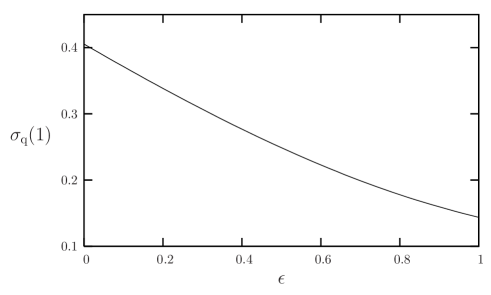
Figure 4: Quenched entropy for the Hamiltonian circuits in graphs with a fraction $\epsilon$ of degree 3 vertices, and $1-\epsilon$ of degree 4.

V.2 In the presence of degree 2 sites in the 2-core

Let us now consider the question of the longest cycles in random graph ensembles with connectivity distribution $q_{k}$ which do not fulfill the condition $q_{0}=q_{1}=q_{2}=0$ we assumed in the previous subsection. We first present simple combinatorial arguments which lead to bounds on $\ell_{\rm max}$ and to an asymptotic expansion when there are very few degree 2 sites in the 2 core, before coming back to the limit $u\to\infty$ of the cavity approach.

V.2.1 Bounds on $\ell_{\rm max}$

Let us call $G_{1}$ a graph drawn at random from such an ensemble, and $G_{2}$ its 2-core, determined for instance by the leaf removal algorithm detailed in App. B. $G_{2}$ has the connectivity distribution $r_{k}$ defined and computed in Sec. III.2 and App. B. The number of sites in the 2-core is $N\ell_{\rm core}$ (cf. Eq. 126), with $\ell_{\rm core}<1$ unless the original graph was deprived of any isolated sites and of leaves (i.e. $q_{0}=q_{1}=0$). This $\ell_{\rm core}$ is clearly an upper bound on $\ell_{\rm max}$, as circuits cannot be longer that the number of available sites in the 2-core.

One can derive a lower bound on $\ell_{\rm max}$ with the following reasoning. From $G_{2}$, the 2-core of $G_{1}$, eliminate recursively sites of degree 2, identifying the two edges which were previously incident to it (see Fig. 5). When all sites of degree 2 have been removed, one ends up with a graph, call it $G_{3}$, on $N(\ell_{\rm core}-r_{2})$ sites, where the minimal connectivity is 3. Using the result of the previous section, this reduced graph typically contains circuits of length $N(\ell_{\rm core}-r_{2})$. Each of the circuits of $G_{3}$ can be unambiguously associated to a circuit of $G_{2}$, reinserting the edges which were simplified during the construction of $G_{3}$. Obviously the reconstructed circuits of $G_{2}$ are longer than the ones of $G_{3}$, hence $l_{\rm lb}=(\ell_{\rm core}-r_{2})$ should be a lower bound for $\ell_{\rm max}$. These bounds have been used under a stronger form in the case of Erdos-Renyi random graphs very close to the percolation threshold (for $c=1+\delta$ with $N^{-1/3}\ll\delta\ll 1$) in Luczak .

One can then wonder if the upper bound is saturated, in other words if the 2-core is Hamiltonian. In general the answer is no, as explained by the following remark. Consider a site of degree strictly greater than 2, surrounded by at least three neighbors of degree 2: obviously, no circuit can go through more than two of these neighbors. As soon as $r_{2}>0$ there will be an extensive number of such forbidden vertices, hence in such a case $\ell_{\rm max}<\ell_{\rm core}$. The equality is possible only if $r_{2}=0$, which was the case investigated in the previous section.

Note that the gap between the lower and upper bound closes when $r_{2}$ vanishes, as the 2-core becomes Hamiltonian in this limit. A conjecture on the behaviour of $\ell_{\rm max}$ in the limit $r_{2}\to 0$ can be formulated as

$$\ell_{\rm max}=\ell_{\rm core}-\sum_{k=3}^{\infty}r_{k}{k\choose 3}\tilde{r}_{1}^{3}+O(\tilde{r}_{1}^{4})\ .$$ (55)

This expression has a very simple interpretation: a forbidden site in the above argument appears if a vertex of degree greater than 3 is surrounded by at least three vertices of degree 2. At the lowest order these forbidden sites are far apart from each other, $N\ell_{\rm max}$ is thus reduced by one unit each time this appears. This conjecture will come out of the cavity analysis of next subsection, we preferred to anticipate it here because of its simple combinatorial interpretation.

Figure 5: A single step of the simplification algorithm (from $G_{2}$ to $G_{3}$) used in Sec. V.2.

Let us exemplify the bounds and the conjecture in two particular cases. Consider ensemble of graphs where a fraction $1-\epsilon$ of vertices have degree $c_{0}\geq 3$, the others being of degree 2, with $0\leq\epsilon<1$. The above bounds and estimation read

$$1-\epsilon\leq\ell_{\rm max}\leq 1\ ,\quad\ell_{\rm max}=1-\frac{4(c_{0}-1)(c_{0}-2)}{3c_{0}^{2}}\epsilon^{3}+O(\epsilon^{4})\ .$$ (56)

As a second example we consider Poissonian random graphs of mean degree $c$, for which the bounds read (cf. Eq. (29))

$$\ell_{\rm lb}=1-(1-\eta)\left(1+c\eta+\frac{1}{2}(c\eta)^{2}\right)\ ,\qquad\ell_{\rm core}=1-(1-\eta)(1+c\eta)\ ,$$ (57)

where $\eta$ is the solution of $\eta=1-\exp(-c\eta)$. In the limit $c\to\infty$ the fraction of degree 2 vertices in the 2-core vanishes, the above conjecture reads then

$$\ell_{\rm max}=1-(c+1)e^{-c}-c^{2}e^{-2c}-\frac{c^{2}}{2}\left(\frac{c^{4}}{3}+3c-1\right)e^{-3c}+O(c^{n}e^{-4c})\ ,$$ (58)

where $n$ is some positive integer. Most of these terms come from the expansion of $\ell_{\rm core}$, the only non-trivial one being $-c^{6}e^{-3c}/6$. This is in agreement with a rigorous result of Frieze Frieze ,

$$1-(1+\delta(c))ce^{-c}\leq\ell_{\rm max}\leq 1-(c+1)e^{-c}\ \quad{\rm with}\ \ \delta(c)\underset{c\to\infty}{\to}0\ .$$ (59)

V.2.2 The large $u$ limit in presence of sites of degree 2

We come back to the cavity approach and investigate the large $u$ limit in this case. The simple ansatz $y\sim xu^{-1/2}$ is not compatible with Eqs. (20,21) any longer, because of the non vanishing value of $\tilde{r}_{1}$. The most natural generalization which allows to close this set of equations is then $y\sim xu^{p-1/2}$, where $p$ is a relative integer (hard field). We denote $V_{p}(x)$ the probability distribution of the evanescent fields $x$ associated to hard fields $p$. For notational simplicity we take the $V_{p}$ to be unnormalized, with $\int_{0}^{\infty}dx\,V_{p}(x)=v_{p}$, and impose the condition $\sum_{p\in\mathbb{Z}}v_{p}=1$. Expanding Eqs. (20,21) with this ansatz, one finds

$$V_{p}(x)=\sum_{k=1}^{\infty}\tilde{r}_{k}\sum_{p_{1},\dots,p_{k}\in\mathbb{Z}^{k}}\delta_{p,e_{k}(p_{1},\dots,p_{k})}\int_{0}^{\infty}dx_{1}\,V_{p_{1}}(x_{1})\dots dx_{k}\,V_{p_{k}}(x_{k})\,\delta(x-h_{k}(p_{1},x_{1},\dots,p_{k},x_{k}))\ .$$ (60)

In order to simplify the expression of $e_{k}$ and $h_{k}$, we shall denote $[n]$ a permutation of the indices which orders the hard fields in decreasing order, $p_{[1]}\geq p_{[2]}\geq\dots p_{[k]}$. Then

$$e_{1}(p_{1})=1+p_{1}\ ,\quad e_{k}(p_{1},\dots,p_{k})=\min(1+p_{[1]},-p_{[2]})\quad{\rm for}\ k\geq 2\ .$$ (61)

We also define

$$d_{k}(p_{1},x_{1},\dots,p_{k},x_{k}) = \begin{cases}1&{\rm if}\ p_{[1]}+p_{[2]}<-1\\ 1+\hat{d}_{k}(p_{1},x_{1},\dots,p_{k},x_{k})&{\rm if}\ p_{[1]}+p_{[2]}=-1\\ \hat{d}_{k}(p_{1},x_{1},\dots,p_{k},x_{k})&{\rm if}\ p_{[1]}+p_{[2]}>-1\end{cases}\ ,$$ (62)

$$\hat{d}_{k}(p_{1},x_{1},\dots,p_{k},x_{k}) = \begin{cases}\underset{i<j|p_{i}=p_{j}=p_{[1]}}{\sum}x_{i}x_{j}&{\rm if}\ p_{[1]}=p_{[2]}\\ x_{[1]}\underset{i|p_{i}=p_{[2]}}{\sum}x_{i}&{\rm if}\ p_{[1]}>p_{[2]}\end{cases}\ ,$$ (63)

in terms of which the evanescent contribution reads

$$h_{1}(p_{1},x_{1})=x_{1}\ ,\quad h_{k}(p_{1},x_{1},\dots,p_{k},x_{k})=\frac{\underset{i|p_{i}=p_{[1]}}{\sum}x_{i}}{d_{k}(p_{1},x_{1},\dots,p_{k},x_{k})}\quad{\rm for}\ k\geq 2\ .$$ (64)

Within this ansatz the logarithmic moments (cf. Eq. (50)) behave as

$$I_{k}(u)\sim J_{k}^{({\rm h})}\ln u+J_{k}\ ,$$ (65)

$$J_{k}^{({\rm h})}=\underset{p_{1},\dots,p_{k}\in\mathbb{Z}^{k}}{\sum}v_{p_{1}}\dots v_{p_{k}}\max(1+p_{[1]}+p_{[2]},0)\ ,$$ (66)

$$J_{k}=\underset{p_{1},\dots,p_{k}\in\mathbb{Z}^{k}}{\sum}\int_{0}^{\infty}dx_{1}\,V_{p_{1}}(x_{1})\dots dx_{k}\,V_{p_{k}}(x_{k})\,\ln d_{k}(p_{1},x_{1},\dots,p_{k},x_{k})\ .$$ (67)

From the behaviour of $f_{\rm q}$ we thus obtain

$$\ell_{\rm max}=\sum_{k=3}^{\infty}r_{k}\left(\frac{k}{2}J_{k-1}^{({\rm h})}-\frac{k-2}{2}J_{k}^{({\rm h})}\right)\ ,\qquad\sigma_{\rm q}(\ell_{\rm max})=\sum_{k=3}^{\infty}r_{k}\left(\frac{k}{2}J_{k-1}-\frac{k-2}{2}J_{k}\right)\ .$$ (68)

Obviously this set of expressions reduces to the ones of Sec. V.1 when all the hard fields are null, which is a solution if and only if $\tilde{r}_{1}=0$.

Let us first discuss the computation of $\ell_{\rm max}$. This quantity can be obtained from the distribution $v_{p}$ of the hard fields, independently of the evanescent ones. Integrating away the evanescent fields in Eq. (60), one obtains:

$$v_{p}=\sum_{k=1}^{\infty}\tilde{r}_{k}\sum_{p_{1},\dots,p_{k}\in\mathbb{Z}^{k}}v_{p_{1}}\dots v_{p_{k}}\delta_{p,e_{k}(p_{1},\dots,p_{k})}\ .$$ (69)

Besides the population dynamics method, a faster and more precise method can be devised to solve this equation. Let us for this purpose define $w_{p}$, the integrated form of the distribution, and $\varphi(x)$ the generating function of the $\tilde{r}_{k}$’s:

$$w_{p}=\sum_{p^{\prime}=-\infty}^{p-1}v_{p}\ ,\quad\varphi(x)=\sum_{k=1}^{\infty}\tilde{r}_{k}x^{k}\ .$$ (70)

One can then rewrite Eq. (69), after a few lines of computation based on the expression of $e_{k}(p_{1},\dots,p_{k})$, under the form

$$\begin{cases}w_{p+1}=1-(1-w_{p})\varphi^{\prime}(w_{-p})\ \\ w_{-p}=1-(1-w_{p+1})\varphi^{\prime}(w_{p+1})+\varphi(w_{-p-1})-\varphi(w_{p+1})\end{cases}\quad{\rm for}\ p\geq 0\ .$$ (71)

It is easy to solve them numerically by iteration (both $w_{-p}$ and $1-w_{p}$ vanish exponentially fast when $p\to+\infty$, a cutoff on $p$ can thus be safely introduced), and to deduce $\ell_{\rm max}$ from the solution $v_{p}$ (see Eqs. (66,68)). We present the results of this procedure for Poissonian graphs in the left panel of Fig. 6, along with the bounds discussed above.

We now sketch the way to compute the expansion of $\ell_{\rm max}$ stated in Eq. (55). In the limit $\tilde{r}_{1}\to 0$, the distribution $v_{p}$ tends to $\delta_{p,0}$. A more precise inspection reveals that $v_{p}=O(\tilde{r}_{1}^{p})$, $v_{-p}=O(\tilde{r}_{1}^{2p})$ for $p>0$. In order to obtain Eq. (55), it is thus enough to find $\{v_{-1},v_{0},v_{1},v_{2},v_{3}\}$ at order $\tilde{r}_{1}^{3}$, in function of the connectivity distribution $\tilde{r}_{k}$. The result follow by collecting the terms of order $\tilde{r}_{1}^{3}$ in Eqs. (66,68). This expansion could be in principle pursued at any higher order, at the price of more tedious computations.

If one is not only interested in the length of the longest circuits, but also in the associated entropy $\sigma_{\rm q}(\ell_{\rm max})$, one has to solve the complete equation (60) on the distribution of both hard and evanescent fields. This is easily done by a population dynamics algorithm, following population of couples $(p,x)$, see the right panel of Fig. 6 for the results in the Poissonian case. However, when the value of $\tilde{r}_{1}$ is too large, there appears an instability in the resolution of Eq. (60). For the sake of definiteness let us consider the Poissonian case and postpone a more general discussion to the next section. For values of $c$ larger than a critical value $c_{\rm s}^{(+)}\approx 2.88$, the evanescent fields distributions converge, whereas below $c_{\rm s}^{(+)}$, the iteration brings some of them towards diverging or vanishing values. The origin of this instability can be traced back to the behaviour of the original messages $y$ at large but finite $u$. A closer inspection of numerically obtained histograms of the $y$’s reveals that in this limit they indeed obey a scaling of the form $y\sim xu^{p-1/2}$, but $p$ is a relative integer only for $c\geq c_{\rm s}^{(+)}$. For lower connectivities, a continuously growing fraction of the hard fields are half-integers. This fraction reaches one at $c_{\rm s}^{(-)}\approx 2.67$, below which all $p$’s are half-integers. If one allows the hard fields to be both integers and half-integers in Eqs. (60,66,67), this instability problem is cured, which allowed us to obtain the (dashed) low connectivity part of the curves in Fig. 6. We shall come back in the next section on the interpretation of this phenomenon.

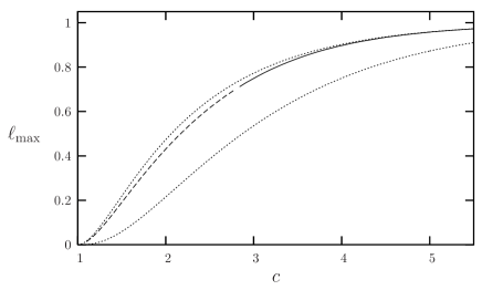
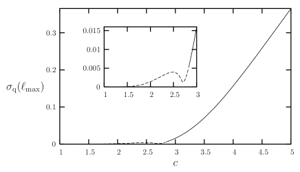
Figure 6: The length of longest cycles in Poissonian graphs of mean connectivity $c$ (left) and the associated quenched entropy (right). Dotted lines in the left panel are the bounds of Eq. (57). The dashed part of the curves corresponds to the regime $c\leq c_{\rm s}^{(+)}$, where we expect the replica symmetry to be broken. The inset of the right figure shows a blow-up for small connectivities, the replica symmetric entropy presents a local maximum (resp. minimum) at $c\approx 2.48$ (resp. $c\approx 2.71$).

VI Stability of the replica-symmetric ansatz

The cavity computations we have presented so far were based on the assumption of replica symmetry (RS), valid if the space of configurations is smooth enough. In disordered systems this assumption can be violated, we shall thus investigate its validity in the present model. More precisely, we consider the local stability of the RS ansatz in the enlarged space of one step replica symmetry breaking (1RSB) order parameters MePa_Bethe (we leave aside the possibility of a discontinuous transition). In the 1RSB setting, the messages $y$ are replaced by probability distributions $Q(y)$ over the states, and the recursion $y\leftarrow g_{k}(y_{1},\dots,y_{k})$ becomes

$$Q(y)\leftarrow\frac{1}{\cal Z}\int dy_{1}Q_{1}(y_{1})\dots dy_{k}Q_{k}(y_{k})\ \delta(y-g_{k}(y_{1},\dots,y_{k}))\ W(y_{1},\dots,y_{k})^{m}\ ,$$ (72)

where $\cal Z$ is a normalization constant, $m$ is the Parisi 1RSB parameter, and $W(\{y_{k\to i}\})$ is a reweighting factor whose explicit form is not needed here. The distributions $Q$ are themselves drawn from a distribution over distributions, ${\cal Q}[Q]$.

The replica symmetric solution studied in the main part of the text is recovered by taking the distributions $Q$ concentrated on a single value $y$. To investigate its local stability, one gives them an infinitesimal variance $v$. Expanding Eq. (72) in the limit of vanishing $v$’s, one obtains the following relation:

$$(y,v)\leftarrow\left(g_{k}(y_{1},\dots,y_{k}),\sum_{j=1}^{k}\left(\frac{\partial g_{k}(y_{1},\dots,y_{k})}{\partial y_{j}}\right)^{2}v_{j}\right)\ .$$ (73)

For the RS solution to be stable against this perturbation, the variances of the 1RSB order parameters should decrease upon iterations of the above relation. This can be studied numerically for any random graph ensemble, by iterating the above relation on a population of couples $(y,v)$, the value of $k$ being drawn from $\tilde{r}_{k}$. The variances $v$ can be initially all taken to 1 (note that Eq. (73) is linear in the $v$’s), in the course of the dynamics the $v$’s are periodically divided by a number $\lambda$, chosen each time to maintain the average value of $v$ constant. After a thermalization phase $\lambda$ converges (in order to gain numerical precision one computes the average over the iterations of $\ln\lambda$), its limit being $>1$ (resp $<1$) if the RS solution is unstable (resp. stable). This method, pioneered in the context of the instability of the 1RSB solution in MoPaRi , can be replaced by the computation of the associated non-linear susceptibility, see for instance BM .

For regular random graphs of connectivity $c$, where all RS messages take the same value $y_{\rm r}(u,c)$ given in Eq. (30), one can readily compute the value of the stability parameter,

$$\lambda_{\rm r}(u,c)=\frac{(2-u(c-1))^{2}}{u^{2}(c-1)^{3}}\ .$$ (74)

It is easy to check that $0\leq\lambda_{\rm r}(u,c)\leq(c-1)^{-1}<1$ when $u$ lies in its allowed range $[u_{\rm m}=(c-1)^{-1},\infty[$, confirming the validity of the RS ansatz. It would have been anyhow surprising to discover an instability in this case where the annealed computation is exact.

Another case which is analytically solvable is the limit $\ell\to 0$ (i.e. $u\to u_{\rm m}$). Indeed, we have seen that the messages scales then as $x(u-u_{\rm m})^{2}$, and it turns out that $\partial g_{k}/\partial y_{i}\to u_{\rm m}$, independently of the rescaled messages $x$. Recalling that $\sum_{k}\tilde{r}_{k}k=\tilde{\mu}_{1}=u_{\rm m}^{-1}$, one finds $\lambda=\tilde{\mu}_{1}^{-1}<1$ in this limit: for any connectivity distribution, the RS ansatz is always stable in the small $\ell$ regime.

All the numerical investigations of $\lambda$ we conducted for ensembles with minimal connectivity 3 suggest that in this case the replica symmetric solution is stable for all values of $u$. Note that here the zero temperature limit of $\lambda$ can be studied directly at the level of evanescent fields, as $\partial g_{k}/\partial y_{i}\to\partial h_{k}/\partial x_{i}$. We thus conjecture that the whole function $\sigma_{\rm q}(\ell)$ computed with the RS cavity method is correct for these ensembles, and in particular the quenched entropy of Hamiltonian circuits $\sigma_{\rm q}(1)$ stated in Eq. (54).

The situation is less fortunate for Poissonian graphs. The reader may have anticipated the appearance of non integer hard fields in the zero temperature limit for mean connectivities lower than $c_{\rm s}^{(+)}$ as an hint of RSB. The datas presented in the left panel of Fig. 7 shows indeed that for small $c$, the stability parameter $\lambda$ crosses 1 when $u$ is increased above some finite value $u_{\rm s}(c)$. This critical value of $u$ increases with the mean connectivity, and an educated guess makes us conjecture that it diverges at $c_{\rm s}^{(+)}$. The rightmost curve for $c=3$ shows indeed $\lambda<1$ for all the values of $u$ we could numerically study. A precise extrapolation of $u_{\rm s}(c)$ turned out however to be rather difficult. Note also that the study directly at $u=\infty$ is largely complicated here by the fact that the hard fields do not take a finite number of distinct values as is often the case in usual optimization problems stab_T0 , but extend on the contrary on all relative integers. In summary, the conjectured scenario is that at high enough connectivities the whole curve $\sigma_{\rm q}(\ell)$, and in particular its zero temperature limit, is correctly described by the RS computation. For lower connectivities there will be a critical length above which replica symmetry breaks down. We also believe that this scenario, sketched in the right part of Fig. 7, is valid not only in the Poissonian case, but for all families of random graph ensembles (with a fastly decaying connectivity distribution) with a control parameter which drives the graphs towards a continuous percolation transition, the fraction of degree 2 sites in the 2-core growing as the transition is approached.

Let us finally propose an interpretation for the occurrence of replica symmetry breaking for the largest circuits in presence of a large fraction of degree 2 sites in the 2 core, by relating it to an underlying extreme value problem extreme . In the discussion of Sec. V.2.1, one could indeed tag the edges $l$ of the reduced graph $G_{3}$ with a strictly positive integer, by counting the number of edges of $G_{2}$ which were collapsed onto $l$. The length of a circuit of $G_{2}$ is thus the weighted length of the corresponding circuit of $G_{3}$, i.e. the sum of the labels on the edges it visits. These weighted lengths are correlated random variables, because of the structural constraint defining a circuit: for a given graph $G_{3}$, not all the sums of $L$ tags correspond to circuits of length $L$. When the fraction of degree 2 site is small enough, these correlations are sufficiently weak for the RS ansatz to treat them correctly, when long chains of degree 2 vertices become too numerous they somehow pin the longest circuits, which cluster in the space of configurations and cause the replica symmetry breaking.

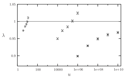
Figure 7: Left: the stability parameter $\lambda$ for Poissonian random graphs, from left to right $c=1.2$, $2$, $3$. Right: Sketched behaviour of the quenched entropy for generic families of random graphs. From top to bottom a control parameter drives the graphs towards a continuous percolation transition, the maximal length of the circuits is reduced. In the neighborhood of the percolation transition replica symmetry breaking takes place for large enough circuits, and should be taken into account to compute the dashed part of the curve.

VII Exhaustive enumerations

We present in this section the results of the numerical experiments we have conducted in order to check our analytical predictions. These experiments are based on the exhaustive enumeration algorithm of Johnson which allows to generate all the circuits of a given graph $G$, and in particular to compute the numbers ${\cal N}_{L}(G)$ of circuits of a given length. This algorithm runs in a time proportional to the total number of circuits, hence exponential in the size of the graphs for the cases we are interested in, which obviously puts a strong limitation on the sizes we have been able to study.

Let us begin with the investigation of the Erdös-Rényi ensembles $G(N,p)$ and $G(N,M)$. In the former, each of the $N(N-1)/2$ potential edges between the $N$ vertices of the graph is present with probability $p$, independently of each other, in the latter a set of $M$ among the $N(N-1)/2$ edges is chosen uniformly at random. With $p=c/N$ and $M=cN/2$, these two ensembles are expected to be equivalent in the large-size limit. In particular the vertex degree distribution converges in both cases to a Poisson law of mean $c$, the cavity computation thus predicts that their typical properties should be the same in the thermodynamic limit. This is not true for the the annealed entropies $\sigma_{\rm a}(\ell;N)=\log(\overline{{\cal N}_{\ell N}})/N$ which are easily computed exactly even at finite sizes, see App. A, and which remain distinct in the thermodynamic limit. In the left part of Fig. 8 we present the annealed and quenched entropies for both ensembles, computed from 10000 graphs of size $N=36$ and mean connectivity $c=3$. The finite size quenched entropy has been estimated using the median of the random variables ${\cal N}_{L}$. The annealed entropies are very different in both ensembles (and in perfect agreement with the computation of App. A), and clearly different from the quenched ones. The striking feature of this plot is the almost perfect coincidence of the median in the two ensembles; this was expected in the thermodynamic limit, but is already very clear at this moderate size. On the right panel of Fig. 8, the quenched entropy is plotted for two graph sizes, along with its extrapolated values in the thermodynamic limit, which agrees with the cavity computation.

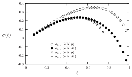
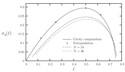
Figure 8: Left: Annealed and quenched entropies for the Erdös-Rényi ensembles $G(N,p)$ and $G(N,M)$ of mean connectivity $c=3$, for graphs of size $N=36$, computed from the mean and the median of ${\cal N}_{L}$ on samples of 10000 graphs. Right: the quenched entropy for $G(N,M)$ at $N=36$, and $N=54$, symbols are the extrapolation in the limit $N\to\infty$ from several values of $N$, solid line is the replica symmetric cavity computation.

As argued above, the difference between annealed and quenched entropies can be also seen in the exponentially larger value of the second moment of ${\cal N}_{L}$ with respect to the square of the first moment. This fact is illustrated in Fig. 9, where the analytic computation of the ratio $\log(\overline{{\cal N}_{L}^{2}}/\overline{{\cal N}_{L}}^{2})/N$ presented in App. A is confronted with its numerical determination.

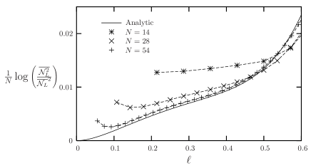
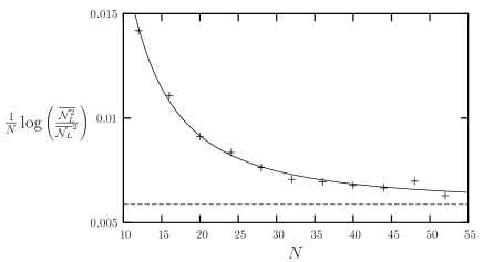
Figure 9: Left: the ratio of the first two moments of ${\cal N}_{L}$ for $G(N,M)$ at $c=3$, the symbols are numerically determined values which converge in the large size limit to the solid line, analytically computed in App. A. Right: finite size analysis for $\ell=1/4$, solid line is a best fit of the form $a+b/N+c/N^{2}$, where $a$ is constrained to its analytic value (dashed line), and the form of the fit is justified in App. A.

We also considered the largest circuits in each graph, of length $L_{\rm max}$ and degeneracy ${\cal N}_{L_{\rm max}}$, and computed the averages $\overline{L_{\rm max}}/N$ and $\overline{\ln{\cal N}_{L_{\rm max}}}/N$ for various connectivities. Their extrapolated values in the thermodynamic limit are compatible with the predictions $\ell_{\rm max}$ and $\sigma_{\rm q}(\ell_{\rm max})$ of the cavity method, within the numerical accuracy we could reach. This is true also for connectivities smaller than $c_{\rm s}^{(+)}$, where we argued above in favor of a violation of the replica symmetry hypothesis: the corrections due to RSB should be smaller than the numerical precision we reached.

Another set of experiments concerned uniformly generated graphs with an equal number of degree 3 and 4 vertices. We checked that the probability for such graphs to be Hamiltonian converges to 1 when increasing their size. The values for the annealed and quenched entropies for the Hamiltonian circuits are too close to be distinguished numerically. However the study of the ratio of the first two moments of ${\cal N}_{N}$ (see Fig. 10) indicates that they should be strictly distinct in the thermodynamic limit.

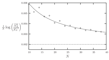
Figure 10: The ratio of the first two moments of ${\cal N}_{N}$ for graphs with an equal fraction of degree 3 and 4 vertices. Solid line is a best fit of the form $a+b/N+c/N^{2}$, with $a\approx 0.002$, as found in App. A.

VIII Conclusions and perspectives

Let us summarize the main results presented in this paper. We have proposed an approximative counting algorithm that runs in a linear time with respects to the size of the graph. We also presented an heuristic method to compute the typical number of circuits in random graph ensembles, which yields a quantitative refinement of Wormald’s conjecture on the typical number of Hamiltonian cycles in ensembles with minimal degree 3 (Eq. (54)) and a new conjecture on the maximal length of circuits in ensembles with a small fraction of degree 2 vertices in their 2 cores (Eq. (55)).

Several directions are opened for future work. First of all we believe that a rigorous proof of Wormald’s conjecture, which seems difficult to reach by variations around the second moment method, could be obtained by statistical mechanics inspired techniques. In recent years there has been indeed a series of mathematical achievements in the formalization of the kind of method used in this article. One line of research is based on Guerra’s interpolation method Guerra , and culminated in Talagrand’s proof of the correctness of the Parisi free-energy formula for the Sherrington-Kirkpatrick model Talagrand . These ideas have also been applied to sparse random graphs in FrLe ; FrLeTo . Alternatively the local weak convergence method of Aldous Aldous has been successfully applied to similar counting problems in random graphs Counting .

There has also been a recent interest MoRi ; PaSl ; ChCh in the corrections to the Bethe approximation for general graphical models. It would be of great interest to implement these refined approximations for the counting problem considered in this paper. This should lead on one hand to a more precise counting algorithm, and on the other hand give access to the finite-size corrections of the quenched entropy. We expect in particular that the difference between circuits and unions of vertex disjoint circuits will become relevant for these corrections.

The convergence in probability of $\log{\cal N}_{L}/N$ expressed by Eq. (17) can a priori be promoted to a stronger large deviation principle: according to the common wisdom, the finite deviations of this quantity from $\sigma_{\rm q}$ are exponentially small. A general method for computing these rate functions has been presented in Olivier and could be of use in the present context. An interesting question could be to compute the exponentially small probability that a random graph is not Hamiltonian in ensembles where typical graphs are so.

In the algorithmic perspective, one could try to take advantage of the local informations provided by the messages. In particular they could be useful to explicitly construct long cycles, in a “belief inspired decimation” fashion SP : most probable edges in the current probability law would be recursively forced to be present, and the BP equations re-runned in the new simplified model.

The neighborhood of the percolation transition should also be investigated more carefully, in particular the effects of replica-symmetry breaking onto the structure of the configuration space.

The case of heavy-tailed (scale-free) degree distributions deserves also further work. The assumption of fast decay we made here is indeed crucial for some of our results: Bianconi and Marsili showed in BiMa that scale-free graphs, even with a minimal connectivity of 3, can fail to have Hamiltonian cycles. Other random graph models (generated by a growing process growing , or incorporating correlations between vertex degrees BiMa2 ) could also been investigated.

Let us finally mention two closely related problems which are currently studied with very similar means. Circuits can be defined as a particular case of $k$-regular graphs, with $k=2$. Replacing the number of allowed edges around any site from 2 to $k$ in Eq. (2), one can similarly study the number of $k$-regular subgraphs in random graph ensemble. The case $k=1$ corresponds to matchings, which was largely studied in the mathematical literature matching ; matching2 and have been reconsidered by statistical mechanics methods in Lenka . The appearance of $k\geq 3$-regular subgraphs in random graphs was first considered in Bollobas_k , see Martin for a statistical mechanics treatment.

Appendix A Combinatorial approach

A.1 Notation and definitions

We collect in this appendix the combinatorial arguments for the computation of the first and second moment of the number of circuits in various random graph ensembles. Let us denote ${\cal N}_{L}(G)$ the number of circuits of length $L$ in a graph $G$, and ${\cal C}_{L}$ the set of circuits of length $L$ in the complete graph of $N$ vertices, its cardinality being

$$|{\cal C}_{L}|={\cal M}_{L}=\frac{1}{2L}\frac{N!}{(N-L)!}\ .$$ (75)

Indeed, choosing such a circuit amounts to select an ordered list of the $L$ vertices it will visit, modulo the orientation and the starting point of the tour. Introducing $\mathbb{I}(H;G)$ the indicator function equal to $1$ if $H$ is a subgraph of $G$, $0$ otherwise, we can write

$${\cal N}_{L}(G)=\sum_{C\in{\cal C}_{L}}\mathbb{I}(C;G)\ .$$ (76)

Let us now describe the random graph ensembles we shall consider in the following. The first two are the classical Erdös-Rényi random graph ensembles. In $G(N,p)$, each of the $N(N-1)/2$ edges is present with probability $p$, independently of the others. In $G(N,M)$, a set of $M$ distinct edges is chosen uniformly at random among the $N(N-1)/2$ possible ones. We shall concentrate on the thermodynamic limit $N\to\infty$, $p=c/N$ and $M=cN/2$ with the mean connectivity $c$ kept finite. In this regime $G(N,p)$ and $G(N,M)$ are essentially equivalent: drawing at random from $G(N,p)$ amounts to draw $M$ from a binomial distribution of parameters $(p,N(N-1)/2)$, and then drawing at random a graph from $G(N,M)$. In the limit described above, the number of edges in $G(N,p)$ is weakly fluctuating around $M=cN/2$. Moreover the degree of a given vertex in the graph converges in both cases to a Poisson random variable of parameter $c$.

For an arbitrary degree distribution $q_{k}$ of mean $c$, one can define the uniform ensemble of graphs obeying this constraint of degree distribution. A practical way of drawing a graph from this ensemble is the so-called configuration model conf_Bollo , defined as follows. Each of the vertices is randomly attributed a degree, in such a way that $Nq_{k}$ vertices have degree $k$ (we obviously skip some technical details MR : $q_{k}$ should be a function of $N$, such that $Nq_{k}$ is an integer). $2k$ half-links goes out of each vertex of degree $k$. Then one generates a random matching of the $cN=2M$ half-links and puts an edge between sites which are matched. In general one obtains in this way a multigraph, i.e. there appear edges linking one vertex with itself, or multiple edges between the same pair of vertices. However, discarding the non-simple graphs leads to an uniform distribution over the simple ones Wormald_review . To compute averages over the graph ensemble, one can thus use the configuration model and condition on the multigraph to be simple. For clarity we shall denote ${\cal N}_{L}^{*}(G)$ the number of circuits in the unconditioned multigraph ensemble. Note also that regular random graphs are a particular case of this ensemble, with $q_{k}=\delta_{k,c}$.

A.2 First moment computations

A.2.1 Generalities

Taking the average over the graphs of Eq. (76) leads to

$$\overline{{\cal N}_{L}(G)}=\sum_{C\in{\cal C}_{L}}\overline{\mathbb{I}(C;G)}={\cal M}_{L}{\cal P}_{L}$$ (77)

for the ensembles we are considering, where the probability ${\cal P}_{L}=\overline{\mathbb{I}(C;G)}$ for a circuit $C\in{\cal C}_{L}$ to be present is independent of $C$. Before inspecting the various cases, let us state the asymptotic behaviour of ${\cal M}_{L}$ in the limit $N,L\to\infty$, $\ell=L/N$ finite, obtained with the Stirling formula:

$${\cal M}_{\ell N} = \frac{1}{N}\frac{1}{2\ell\sqrt{1-\ell}}N^{L}e^{N(-h(1-\ell)-\ell)}(1+O(N^{-1}))\quad\mbox{for}\ 0<\ell<1\ ,$$ (78)

$${\cal M}_{N} = \frac{1}{\sqrt{N}}\sqrt{\frac{\pi}{2}}N^{N}e^{-N}(1+O(N^{-1}))\ .$$ (79)

In the first formula we have introduced the function $h(x)=x\ln x$.

A.2.2 Erdos-Renyi ensembles

In $G(N,p)$ the probability ${\cal P}_{L}$ has a very simple expression, ${\cal P}_{L}=(c/N)^{L}$. The mean number of circuits thus reads

$$\overline{{\cal N}_{L}(G)}=\frac{1}{2L}\frac{N!}{(N-L)!}\left(\frac{c}{N}\right)^{L}=\frac{1}{N}\frac{1}{2\ell\sqrt{1-\ell}}e^{N\sigma(\ell)}(1+O(N^{-1}))\ ,$$ (80)

where the first expression is valid for any $N,L$, and the second one has been obtained in the thermodynamic limit with $0<\ell<1$ The annealed entropy for this first ensemble is:

$$\sigma(\ell)=-(1-\ell)\ln(1-\ell)+\ell((\ln c)-1)\ .$$ (81)

Note that if $\ell=1$, the algebraic prefactor in (80) is slightly different,

$$\overline{{\cal N}_{N}(G)}=\frac{1}{\sqrt{N}}\sqrt{\frac{\pi}{2}}e^{N((\ln c)-1)}(1+O(N^{-1}))\ .$$ (82)

In $G(N,M)$ the probability ${\cal P}_{L}$ reads

$${\cal P}_{L}=\frac{\left({N\choose 2}-L\right)!}{\left({N\choose 2}\right)!}\frac{M!}{(M-L)!}\ .$$ (83)

Obviously this expression has a meaning only for $L\leq M$, as there cannot be circuits longer than the total number of edges. This gives an exact expression for $\overline{{\cal N}_{L}(G)}={\cal M}_{L}{\cal P}_{L}$ for any $N$ and $L\leq\min(N,M)$. The expansion in the thermodynamic limit with $0<\ell<\min(1,c/2)$ leads to

$$\overline{{\cal N}_{L}(G)}=\frac{1}{N}\frac{e^{\ell(\ell+1)}}{2\ell\sqrt{1-\ell}\sqrt{1-\frac{2\ell}{c}}}e^{N\sigma(\ell)}(1+O(N^{-1}))\ .$$ (84)

with the annealed entropy

$$\sigma(\ell)=-(1-\ell)\ln(1-\ell)+\left(\ell-\frac{c}{2}\right)\ln\left(1-\frac{2\ell}{c}\right)+\ell((\ln c)-2)\ .$$ (85)

Again the different algebraic prefactor in (84) can be easily computed also for $\ell=\min(1,c/2)$.

Let us now make a few comments on these results. First, when $c<1$, both annealed entropies are negative for all values of $\ell>0$ where they are well defined. Consequently $\overline{{\cal N}_{L}(G)}$ is exponentially small in the thermodynamic limit, and thanks to the so-called Markov inequality (or first moment method) valid for positive integer random variables,

$${\rm Prob}[{\cal N}_{L}(G)>0]\leq\overline{{\cal N}_{L}(G)}\ ,$$ (86)

with high probability there are no circuits of extensive lengths in these graphs. This could be expected: the percolation transition occurs at $c=1$, in this non percolated regime the size of the largest component is of order $\ln N$, and thus extensive circuits cannot be present.

As a second remark, let us note that for $c>1$, the annealed entropy of the first ensemble is strictly positive for $\ell\in]0,\ell_{\rm a}(c)[$, with $\ell_{\rm a}(c)$ an increasing function which reaches the value $1$ in $c=e$. The average number of such circuits is in consequence exponentially large. However one can easily convince oneself that this cannot be the typical behaviour. Indeed, it turns out that $\ell_{\rm a}(c)$ is larger than the typical number of vertices in the 2-core of the graphs $\ell_{\rm core}(c)$. When $\ell$ belongs to the interval $]\ell_{\rm core}(c),\ell_{\rm a}(c)[$, typically the graphs cannot contain circuits of $L=\ell N$ edges, however an exponentially small fraction of the graphs have 2-core larger than their typical sizes. These untypical graphs contribute with an exponential number of circuits to the annealed mean $\overline{{\cal N}_{L}(G)}$, which is in consequence not representative of the typical behaviour of the ensemble.

Finally, let us underline that the annealed entropies (81,81) for the two ensembles are definitely different. For instance, in the second ensemble, the entropy is defined only for $\ell\leq c/2$: the number of edges in the graph being fixed at $M=Nc/2$, no circuits can be longer than the number of edges. On the contrary, in the first ensemble, arbitrary large deviations of the number of edges from its typical value are possible, even if with an exponential small probability.

A.2.3 Arbitrary connectivity distribution and regular

The expectation of the number of circuits of length $L$ in the multigraph ensemble extracted with the configuration model was presented in BiMa . For the sake of completeness and to make the study of the second moment simpler we reproduce the argument here. In this case one has

$${\cal P}_{L}=\frac{1}{{N\choose L}}\left(\underset{\{L_{k}\}}{\sum}\prod_{k=2}^{\infty}{Nq_{k}\choose L_{k}}(k(k-1))^{L_{k}}\right)\frac{(cN-2L-1)!!}{(cN-1)!!}\ ,$$ (87)

where the sum is over $L_{2},L_{3},\dots$ positive integers constrained by $\sum_{k=2}^{\infty}L_{k}=L$, and we used the classical notation $(2p-1)!!=(2p-1)(2p-3)\dots 1$. The $L_{k}$’s are the number of sites of degree $k$ in the circuit, which are to be distributed among the $Nq_{k}$ sites of degree $k$. The term $(k(k-1))^{L_{k}}$ accounts for the choice of the half links around each site, and finally the ratio of the double factorials is the probability that the matching of half-links contains the desired configuration. Introducing the integral representation of the Kronecker symbol, $\delta_{n}=\oint(d\theta/2i\pi)\theta^{-n-1}$, where $\theta$ is a complex variable integrated along a closed path around the origin, this expression can be simplified in

$${\cal P}_{L}=\frac{1}{{N\choose L}}\frac{(cN-2L-1)!!}{(cN-1)!!}\oint\frac{d\theta}{2i\pi}\theta^{-L-1}\prod_{k=2}^{\infty}(1+\theta k(k-1))^{Nq_{k}}\ .$$ (88)

In the thermodynamic limit the integral can be evaluated by the saddle-point method, combining the expansion with the one of ${\cal M}_{L}$ yields

$$\overline{{\cal N}_{L}^{*}(G)} \doteq e^{N\sigma(\ell)}\ ,$$ (89)

$$\sigma(\ell) = \frac{1}{2}h(c-2\ell)-\frac{1}{2}h(c)+h(\ell)+\underset{\theta}{{\rm ext}}\left[\sum_{k=2}^{\infty}q_{k}\ln(1+k(k-1)\theta)-\ell\ln\theta\right]\ ,$$ (90)

where here and in the following $\doteq$ stands for equivalence upto subexponential terms, i.e. $x_{N}\doteq y_{N}$ means $(1/N)\log(x_{N}/y_{N})\to 0$ as $N\to\infty$.

In the regular case one has

$${\cal P}_{L}=(c(c-1))^{L}\frac{(cN-2L-1)!!}{(cN-1)!!}\ ,$$ (91)

from which the prefactors are more easily computed

$$\overline{{\cal N}_{L}^{*}(G)} = \frac{1}{N}\frac{1}{2\ell\sqrt{1-\ell}}e^{N\sigma(\ell)}(1+O(N^{-1}))\quad{\rm for}\ 0<\ell<1\ ,$$ (92)

$$\overline{{\cal N}_{N}^{*}(G)} = \frac{1}{\sqrt{N}}\sqrt{\frac{\pi}{2}}e^{N\sigma(1)}(1+O(N^{-1}))\ ,$$ (93)

$$\sigma(\ell) = -h(1-\ell)-\frac{1}{2}h(c)+\frac{1}{2}h(c-2\ell)+\ell\ln(c(c-1))\ .$$ (94)

Moreover the conditioning on the multigraph being simple can be explicitly done in the regular case Garmo , thanks to the relative concentration of ${\cal N}_{L}^{*}(G)$. This yields

$$\frac{\overline{{\cal N}_{L}(G)}}{\overline{{\cal N}^{*}_{L}(G)}}\to\exp\left[\frac{(c-2)\ell}{c-2\ell}\left(1+\frac{c(1-\ell)}{c-2\ell}\right)\right]\quad{\rm for}\ 0<\ell\leq 1\ .$$ (95)

We checked that the numerical findings of MaMo were in perfect agreement with these exact results.

Note that in the regular case, this conditioning modifies the value of $\overline{{\cal N}^{*}_{L}(G)}$ only by a constant factor, thus the annealed entropy is the same in the graph and in the multigraph ensemble. It is not clear to us whether this fact should remain true for arbitrary connectivity distributions.

A.3 Second moment computations

A.3.1 Generalities

We now turn to the computation of the second moment of the number of circuits, which has been inspired by Garmo . Taking the square of Eq. (76) and averaging over the ensemble leads to

$$\overline{{\cal N}_{L}^{2}(G)}=\sum_{C_{1},C_{2}\in{\cal C}_{L}}\overline{\mathbb{I}(C_{1};G)\mathbb{I}(C_{2};G)} = \overline{{\cal N}_{L}(G)}+\sum_{C_{1}\neq C_{2}\in{\cal C}_{L}}\overline{\mathbb{I}(C_{1};G)\mathbb{I}(C_{2};G)}$$ (96)

$$= \overline{{\cal N}_{L}(G)}+\sum_{X,Y,Z}{\cal M}_{LXYZ}{\cal P}_{LXYZ}\ .$$ (97)

We have indeed isolated the term $C_{1}=C_{2}$ in the sum, which is readily computed, from the off-diagonal terms. The last expression is more easily understood after having a look at Fig. 11, where we sketched the shape of the union of two distinct circuits. This pattern is characterized by $X$, the number of common paths shared by $C_{1}$ and $C_{2}$, $Y$, the number of edges in these paths, and $Z$, the number of vertices which belongs to both circuits but are not neighbored by any common edge. One finds $2X$ vertices at the extremities of the common paths, $Y-X$ vertices in the interior of the common paths, hence $X+Y+Z$ vertices belong to both circuits, $N-2L+X+Y+Z$ to none of them. In consequence the sum is over $X,Y,Z$ non-negative integers subject to the constraints:

$$2L-N\leq X+Y+Z\leq L\ ,\quad X\leq Y\ ,\quad X=0\Rightarrow Y=0\ .$$ (98)

${\cal M}_{LXYZ}$ is the number of pairs of distinct circuits of the complete graph whose union has the characteristics $(X,Y,Z)$, and ${\cal P}_{LXYZ}$ is the (ensemble-dependent) probability that such pattern appears in a random graph. Let us show that

$${\cal M}_{LXYZ}=\frac{1}{4}2^{X}\frac{N!\ ((L-Y-1)!)^{2}}{X!\ Z!\ ((L-X-Y-Z)!)^{2}\ (N-2L+X+Y+Z)!}\ {Y-1\choose X-1}\ ,$$ (99)

where the combinatorial factor ${-1\choose-1}$ is by convention set to $1$. To construct such a pattern, one has to choose among the $N$ vertices those which are in $C_{1}$ but not in $C_{2}$, in $C_{2}$ but not in $C_{1}$ (both of these categories contain $L-X-Y-Z$ vertices), those in the common paths ($X+Y$) and those shared by the circuits but with no adjacent common edges ($Z$). This can be done in

$$\frac{N!}{Z!\ (X+Y)!\ ((L-X-Y-Z)!)^{2}\ (N-2L+X+Y+Z)!}$$ (100)

distinct ways.

Let us call $n_{i}$ the number of common paths of $i$ edges, for $1\leq i\leq L-1$, which obey the constraints $\sum_{i}n_{i}=X$ and $\sum_{i}in_{i}=Y$. The $X+Y$ sites can be distributed into such an unordered set of unorientated paths in

$$\frac{(X+Y)!}{2^{X}}\frac{1}{\prod_{i=1}^{L-1}n_{i}!}$$ (101)

distinct ways. We have to sum this expression on the values of $n_{i}$ satisfying the above constraints. By picking up the coefficient of $t^{Y}$ in

$$(t+t^{2}+\dots+t^{L-1})^{X}=\sum_{n_{1},\dots,n_{L-1}}\frac{X!}{\prod_{i=1}^{L-1}n_{i}!}t^{\sum_{i}in_{i}}\delta_{X,\sum_{i}n_{i}}=t^{X}\left(\frac{1-t^{L-1}}{1-t}\right)^{X}\ ,$$ (102)

one finds that

$$\sum_{n_{1},\dots,n_{L-1}}\frac{1}{\prod_{i=1}^{L-1}n_{i}!}\delta_{X,\sum_{i}n_{i}}\delta_{Y,\sum_{i}in_{i}}=\frac{1}{X!}{Y-1\choose X-1}\ .$$ (103)

When $X=Y=0$ this factor should be one, in agreement with the above convention.

Finally $C_{1}$ is formed by choosing an ordered list of the $L-X-Y-Z$ vertices which belongs only to it, the $Z$ isolated common vertices, and of the $X$ orientated common paths, modulo the starting point and the global orientation of this tour, hence a factor

$$\frac{(L-Y-1)!}{2}2^{X}\ ,$$ (104)

and the same arises when constructing $C_{2}$. Eq. (99) is obtained by multiplying the various contributions.

In the thermodynamic limit with $(x,y,z)=(X/N,Y/N,Z/N)$ kept finite, Stirling formula yields

$${\cal M}_{LXYZ} \doteq N^{N(2\ell-y)}\exp[Nm(l,x,y,z)]\ ,$$ (105)

$$m(l,x,y,z) = y-2\ell+x\ln 2-2h(x)+h(y)-h(z)-h(y-x)$$ (106)

$$+ 2h(\ell-y)-2h(l-x-y-z)-h(1-2\ell+x+y+z)\ .$$

Figure 11: The union of two circuits. The vertices of $C_{1}$ are on and above the horizontal central line, those of $C_{2}$ on and below. In this drawing $L=13$, $X=3$, $Y=6$, $Z=1$, $n_{1}=n_{2}=n_{3}=1$.

A.3.2 Erdos-Renyi ensembles

For both $G(N,p)$ and $G(N,M)$ ensembles, the probability ${\cal P}_{LXYZ}$ depends only on the number of edges present in the union of the two circuits, ${\cal P}_{LXYZ}={\cal P}_{2L-Y}$. For the non trivial range of parameters $\ell,c$ where the first moment is exponentially large, the first term in Eq. (97) can be neglected. The sum over $(X,Y,Z)$ can be evaluated with the saddle-point method, yielding

$$\overline{{\cal N}_{L}^{2}(G)}\doteq\exp[N\tau(\ell)]\ ,\quad\tau(\ell)=\underset{y}{\max}[p(2\ell-y)+\widehat{m}(\ell,y)]\ ,$$ (107)

where

$$p(\ell)=\begin{cases}\ell\ln c&{\rm for}\ G(N,p)\\ \frac{1}{2}h(c)-\frac{1}{2}h(c-2\ell)-\ell&{\rm for}\ G(N,M)\end{cases}\ ,$$ (108)

and we introduced

$$\widehat{m}(\ell,y) = \underset{x,z}{\max}\ m(\ell,x,y,z)$$ (110)

$$= -2h(1-\ell)+y-2\ell+h(y)$$

$$+\underset{x}{\max}\ \left[x\ln 2-2h(x)+h(1-x-y)-h(y-x)+2h(\ell-y)-2h(l-x-y)\right]\ .$$

The range of parameters in the various optimizations are such that $2\ell-1\leq x+y+z\leq\ell$. The step between Eqs. (110) and (110) amounts to maximize $m$ over $z$, which can be done analytically. It is then very easy to determine the function $\widehat{m}(\ell,y)$ numerically. Finally, defining $S(\ell)=\tau(\ell)-2\sigma(\ell)$, we determined numerically this function (see Fig. 9) and found that $S>0$ for all parameters such that $\sigma>0$: the second moment of ${\cal N}_{L}(G)$ is then exponentially larger than the square of the first moment, which forbids the use of the second moment method to determine the typical value of ${\cal N}_{L}$.

A.3.3 Arbitrary connectivity distribution and regular

The computation of ${\cal P}_{LXYZ}$ in the configuration model can be done similarly to the one of ${\cal P}_{L}$ (cf. Eq. (87)). To simplify notations let us define $U=2L-3X-Y-2Z$, $V=2X$, and the multinomial coefficient

$${N\choose U,V,Z}=\frac{N!}{U!V!Z!(N-U-V-Z)!}\ ,$$ (111)

for $U+V+Z\leq N$. We also use $(k)_{n}=k(k-1)\dots(k-n+1)$. With these conventions one finds

$${\cal P}_{LXYZ}=\frac{1}{{N\choose U,V,Z}}\left(\underset{\{U_{k},V_{k},Z_{k}\}}{\sum}\prod_{k=2}^{\infty}{Nq_{k}\choose U_{k},V_{k},Z_{k}}(k)_{2}^{U_{k}}(k)_{3}^{V_{k}}(k)_{4}^{Z_{k}}\right)\frac{(cN-2(2L-Y)-1)!!}{(cN-1)!!}\ .$$ (112)

Indeed, $U$ (resp. $V$, $Z$) is the number of vertices with two (resp. three, four) half-edges involved in the pattern, and $(U_{k},V_{k},Z_{k})$ the number of such vertices among the ones of degree $k$. In consequence the sum is over non-negative integers with $V_{2}=Z_{2}=Z_{3}=0$, $U_{k}+V_{k}+Z_{k}\leq N_{k}$, and $\sum_{k}U_{k}=U$, $\sum_{k}V_{k}=V$, $\sum_{k}Z_{k}=Z$. These last three constraints can be implemented using the complex integral representation of Kronecker’s delta, themselves evaluated by the saddle point method in the thermodynamic limit:

$${\cal P}_{LXYZ} \doteq N^{Y-2L}\exp[Np(\ell,x,y,z)]\ ,$$ (113)

$$p(\ell,x,y,z) = \frac{1}{2}h(c-4\ell+2y)-\frac{1}{2}h(c)+2\ell-y+h(2\ell-3x-y-2z)+h(2x)+h(z)+h(1-2\ell+x+y+z)$$

$$+ \underset{\theta_{1},\theta_{2},\theta_{3}}{{\rm ext}}\left[\sum_{k=2}^{\infty}q_{k}\ln(1+(k)_{2}\theta_{1}+(k)_{3}\theta_{2}+(k)_{4}\theta_{3})-(2\ell-3x-y-2x)\ln\theta_{1}-2x\ln\theta_{2}-z\ln\theta_{3}\right]\ .$$

Once this function has been determined for a given degree distribution, the exponential order of $\overline{{\cal N}_{L}^{*2}(G)}$ can be computed as

$$\overline{{\cal N}_{L}^{*2}(G)}\doteq\exp[N\tau(\ell)]\ ,\quad\tau(\ell)=\underset{x,y,z}{\max}[p(\ell,x,y,z)+m(\ell,x,y,z)]\ ,$$ (114)

where $m$ is given in Eq. (106).

In the regular case, the maximization over the 6 parameters can be performed analytically, and yields $\tau(\ell)=2\sigma(\ell)$ Garmo , proving the concentration (at the exponential order) of ${\cal N}_{L}(G)$ around its mean. We expect that for any (fastly decaying) connectivity distribution not strictly concentrated on a single integer, $\tau(\ell)>2\sigma(\ell)$ when $\sigma(\ell)>0$. A proof of this conjecture would be a quite painful exercise in analysis that we did not undertake. We however verified numerically this statement for the Hamiltonian circuits of random graphs with an equal mixture of vertices of degree 3 and 4, yielding $\tau(1)-2\sigma(1)\approx 0.002$.

We have been rather loose in treating the algebraic prefactor hidden in $\doteq$ for the various expressions of $\overline{{\cal N}_{L}^{2}(G)}$. However it is rather simple to determine the power of $N$ in this prefactor, collecting the contributions which arise from the Stirling expansions, the transformation of sums into integrals, and the evaluation of the latter with the saddle point method. This leads to

$$\frac{\overline{{\cal N}_{L}^{2}(G)}}{\overline{{\cal N}_{L}(G)}^{2}}={\rm cst}\ (1+O(N^{-1}))\exp[N(\tau(\ell)-2\sigma(\ell))]\ ,$$ (115)

as we observed numerically in Sec. VII.

Note also that some informations on the structure of the space of configurations can be obtained from this kind of computations. The average number of pairs of circuits at a given “overlap” (number of common edges) is indeed obtained from the second moment computations if the parameter $y$ is kept fixed.

A.4 On the union of vertex disjoint circuits

In the statistical mechanics treatment of the main part of the text we used a model which counts the number ${\cal N}^{\prime}_{L}(G)$ of subgraphs of $G$ made of the union of vertex disjoint circuits of total length $L$. We want to show in this appendix that, at the leading exponential order, the average of ${\cal N}^{\prime}_{L}(G)$ equals the one of ${\cal N}_{L}(G)$ in the various ensembles considered in this appendix. Let us denote ${\cal C}^{\prime}_{L}$ the set of subgraphs of the complete graph on $N$ vertices made of unions of vertex disjoint circuits of total length $L$, and ${\cal M}^{\prime}_{L}$ its cardinality. As such subgraphs are still made of $L$ edges connecting $L$ vertices, $\overline{{\cal N}^{\prime}_{L}(G)}={\cal M}^{\prime}_{L}{\cal P}_{L}$, where the probability ${\cal P}_{L}$ is the one defined previously for the computation of ${\cal N}_{L}(G)$. Let us define ${\cal M}^{\prime}_{L,A}$ the cardinality of the subset of ${\cal C}^{\prime}_{L}$ where the subgraphs are made of $A$ disjoint circuits. A short reasoning leads to

$${\cal M}^{\prime}_{L,A}=\frac{N!}{(N-L)!}\frac{1}{2^{A}}\underset{A_{3},\dots,A_{L}}{\sum}\frac{1}{\prod_{i=3}^{L}A_{i}!i^{A_{i}}}\ \delta_{\sum_{i}A_{i},A}\ \delta_{\sum_{i}iA_{i},L}\ ,$$ (116)

where the integers $A_{i}$ are the number of circuits of length $i$ in the subgraph. From this expression it is easy to check that ${\cal M}^{\prime}_{L,1}={\cal M}_{L}$, and that as long as $A$ is finite in the thermodynamic limit, ${\cal M}^{\prime}_{L,A}\doteq{\cal M}_{L}$. More precisely, one can show that the leading behaviour of ${\cal M}^{\prime}_{L}=\sum_{A}{\cal M}^{\prime}_{L,A}$ is not modified by contributions with $A$ growing with $N$. Indeed,

$$\frac{{\cal M}^{\prime}_{L}}{{\cal M}_{L}}=2L\ [t^{L}]\ \exp\left[\frac{1}{2}\left(\frac{t^{3}}{3}+\dots\frac{t^{L}}{L}\right)\right]\ ,$$ (117)

where $[t^{x}]f(t)$ denotes the coefficient of order $x$ in the series expansion of $f(t)$. Evaluating the right hand side with the saddle point method when $L\to\infty$, one can conclude that ${\cal M}^{\prime}_{L}\doteq{\cal M}_{L}$ and from the above remark $\overline{{\cal N}^{\prime}_{L}(G)}\doteq\overline{{\cal N}_{L}(G)}$. As far as annealed computations are concerned, the distinction between circuits of (extensive) length $L$ and union of disjoint circuits of total length $L$ does not modify the entropy. The hypothesis made in the main part of the text is that this remains true for the quenched computations.

Appendix B Analysis of the leaf removal algorithm on random graphs with arbitrary connectivity distribution

We want to justify in this appendix the geometric interpretation of the null messages elimination we gave in Sec. III.2. Consider a random graph drawn uniformly among the ones with the connectivity distribution $q_{k}$. The 2-core of a graph is the largest subgraph in which all vertices have connectivity at least two. It can be determined using the following leaf removal algorithm, which reduces iteratively the graph. At each time step, if there is at least one vertex of degree 1, choose randomly one of them, and remove the unique edge to which it belongs. When there is no vertex of degree 1, the algorithm stops. At this point either all the edges have been removed and one is left with $N$ isolated vertices, or there remains some isolated vertices and a subgraph in which all vertices have at least degree 2, i.e. the 2-core of the initial graph.

One can define more generally the $q$-core of a graph as the largest subgraph with minimal degree $q$. For Erdös-Rényi random graphs, the thresholds for the appearance of giant $q$-cores have been obtained in PiSpWo . These results have been recently extended to random graphs with arbitrary connectivity distributions in FeRa , this appendix can thus be viewed as an informal presentation of these mathematical works, with the emphasis put on the quantitative results instead of the mathematical rigor (see also kcore_Doro ; kcore_Doro2 for an heuristic derivation in the arbitrary connectivity distributions case, and kcore_Riordan ; kcore_Janson for new mathematical treatments of the problem). In the following we shall study the behaviour of the leaf removal algorithm through differential equations for the evolution of the average connectivity distribution along the execution of the leaf removal. This method is widely used in mathematics and computer science, see in particular Wormald_diff for a general presentation, and a detailed derivation of the equations (120).

We shall denote $T$ the number of steps (elimination of one edge) already performed by the algorithm, and $t=T/N$ the reduced time variable. Let us call $R_{k}(t)=Nr_{k}(t)$ the average (over the choice of the initial graph and the random decisions taken by the algorithm) number of sites of connectivity $k$ in the residual graph obtained after $Nt$ time steps of the algorithm. The initial condition reads obviously $r_{k}(t=0)=q_{k}$. If one calls $\tilde{r}_{k}(t)$ the probability that the neighbor of the selected degree 1 vertex has connectivity $k+1$, the average evolution of the $R$’s during the time-step $t\to t+1/N$ reads

$$R_{k}(t+1/N)-R_{k}(t)=\delta_{k,0}-\delta_{k,1}+\sum_{k^{\prime}=0}^{\infty}\tilde{r}_{k^{\prime}}(t)[-\delta_{k,k^{\prime}+1}+\delta_{k,k^{\prime}}]\ .$$ (118)

To close this set of equations we have to express the offspring probabilities $\tilde{r}_{k}(t)$ in terms of the connectivity distribution $r_{k}(t)$. As the graph is sequentially exposed by the algorithm, the residual graph at time $t$ is still uniformly distributed according to the connectivity distribution $r_{k}(t)$, hence

$$\tilde{r}_{k}(t)=\frac{(k+1)r_{k+1}(t)}{\sum_{k}kr_{k}(t)}=\frac{(k+1)r_{k+1}(t)}{c-2t}\ .$$ (119)

In the last equality $c$ is the initial mean connectivity $\sum_{k}kq_{k}$, which is reduced by $2/N$ at each time-step. In the thermodynamic limit the discrete time relations (118) become ordinary differential equations,

$$\dot{r}_{0}(t) = 1+\frac{r_{1}(t)}{c\eta(t)^{2}}\ ,$$

$$\dot{r}_{1}(t) = -1-\frac{r_{1}(t)}{c\eta(t)^{2}}+\frac{2r_{2}(t)}{c\eta(t)^{2}}\ ,$$

$$\dot{r}_{k}(t) = -\frac{kr_{k}(t)}{c\eta(t)^{2}}+\frac{(k+1)r_{k+1}(t)}{c\eta(t)^{2}}\quad{\rm for}\ k\geq 2\ .$$ (120)

where dotted quantities are derivatives with respects to time, and we introduced the notation $\eta(t)=\sqrt{1-\frac{2t}{c}}$.

For simplicity let us first assume the existence of a cutoff $k_{\rm m}$ in the original distribution $q_{k}$, $q_{k}=0$ for $k>k_{\rm m}$. As the leaf removal procedure never increases the connectivity of one site, this cutoff remains present in $r_{k}(t)$ for all times. The equations of rank $k_{\rm m}$ in the hierarchy (120) is then closed on $r_{k_{\rm m}}$. Using the fact that $\dot{\eta}(t)=-1/(c\eta(t))$, it can be written as

$$\dot{r}_{k_{\rm m}}(t)=-k_{\rm m}\frac{\dot{\eta}(t)}{\eta(t)}r_{k_{\rm m}}(t)\ ,$$ (121)

and easily integrated with the initial condition $r_{k_{\rm m}}(t=0)=q_{k_{\rm m}}$ as

$$r_{k_{\rm m}}(t)=q_{k_{\rm m}}\eta(t)^{k_{\rm m}}\ .$$ (122)

Now one can prove by a decreasing recurrence on $k$ from $k_{\rm m}$ down to 2 that

$$r_{k}(t)=\sum_{n=k}^{k_{m}}q_{n}{n\choose k}\eta(t)^{k}(1-\eta(t))^{n-k}$$ (123)

solves the hierarchy of equations (120). Note also that the initial conditions $r_{k}(0)=q_{k}$ are enforced by Eq. (123) as $\eta(0)=1$. Once $r_{k}(t)$ has been computed for $k\geq 2$, the equation on $r_{1}$ yields

$$r_{1}(t)=-c\,\eta(t)(1-\eta(t))+\sum_{n=1}^{k_{m}}n\,q_{n}\,\eta(t)(1-\eta(t))^{n-1}\ .$$ (124)

Finally $r_{0}(t)$ can be obtained from the normalization condition of the $r_{k}$’s.

We introduced the cutoff $k_{\rm m}$ to have an explicit starting point of the downwards recurrence on $k$. However, the expression (123) formally solves the hierarchy of equations (120) even for unbounded distributions $q_{k}$, we shall therefore send the cutoff to infinity from now on, assuming that all the sums remain convergent.

The 2-core is found when the leaf-removal algorithm stops, at the smallest time $t_{*}$ for which the number of degree 1 vertices vanishes, $r_{1}(t_{*})=0$. This equation always admits $t_{*}=c/2$ as a solution (the graph has then been emptied), however if there is a smaller solution the 2-core is non trivial and the algorithm stops before having removed all edges. Calling $\eta=\eta(t_{*})$, one obtains if $\eta>0$ :

$$1-\eta=\sum_{k=1}^{\infty}\frac{kq_{k}}{c}(1-\eta)^{k-1}=\sum_{k=0}^{\infty}\tilde{q}_{k}(1-\eta)^{k}\ ,$$ (125)

which is nothing but Eq. (25) on the fraction of non vanishing messages obtained in the main part of the text. The confirmation of the interpretation given in Sec. III.2 follows easily:

• the number of edges in the 2-core is equal to the initial number of edges minus the number of steps performed by the algorithm before stopping, $M_{\rm core}=M-Nt_{*}=M\eta^{2}$.

• the distribution of the connectivities of the sites in the 2-core is $r_{k}(t_{*})$, as expected from Eq. (27).

For completeness we also give the number of sites in the 2-core:

$$N_{\rm core}=N\ell_{\rm core}\ ,\qquad\ell_{\rm core}=\sum_{k=2}^{\infty}r_{k}(t_{*})=1-\sum_{k=0}^{\infty}q_{k}(1-\eta)^{k}-c\eta(1-\eta)\ .$$ (126)

As it should, this number is smaller than the size of the giant component, which reads MR ; NeStWa :

$$N_{\rm giant}=N\left(1-\sum_{k=0}^{\infty}q_{k}(1-\eta)^{k}\right)\ .$$ (127)

Moreover the fraction of sites which are in the giant component but out of the 2-core is proportional to $\eta(1-\eta)$. Indeed, the corresponding edges bear exactly one non null directed message, in the formalism of Sec. III.2: if both messages were non null the edge would be in the 2-core, if both vanished the edge would be out of the giant component.

Appendix C An alternative derivation of $\ell_{\rm max}=1$ when the minimal connectivity is 3

This appendix presents, as a consistency check, another derivation of the identity $\ell_{\rm max}=1$ for random graph ensemble with minimal connectivity of 3. In the main part of the text (Sec. V.1), we obtained it by inspection on the behaviour of the free-energy in the large $u$ limit, because of the absence of hard fields. There exists however another expression of $\ell_{\rm max}$, in terms of the distribution of evanescent fields, obtained by taking the large $u$ limit in Eq. (23):

$$\ell_{\rm max}=\frac{c}{2}\int_{0}^{\infty}dx_{1}\,V_{0}(x_{1})\,dx_{2}\,V_{0}(x_{2})\frac{x_{1}x_{2}}{1+x_{1}x_{2}}\ .$$ (128)

Let us introduce the following functional of any probability distribution law $A$,

$$F_{k}[A](x)=\int_{0}^{\infty}dx_{1}\,A(x_{1})\dots dx_{k}\,A(x_{k})\,\delta(x-h_{k}(x_{1},\dots,x_{k}))\ ,$$ (129)

such that Eq. (52) can be rewritten in a compact way as $V_{0}=\sum_{k}\tilde{q}_{k}F_{k}[V_{0}]$, and a bilinear form on the space of probability distribution functions,

$$\langle A,B\rangle=\int_{0}^{\infty}dx\,dy\,A(x)B(y)\frac{xy}{1+xy}\ .$$ (130)

Consider now this form with its arguments being a distribution $A$ and its image through the functional $F_{k}$:

$$\langle A,F_{k}[A]\rangle=\int_{0}^{\infty}dx_{0}\,A(x_{0})\,dx_{1}\,A(x_{1})\dots dx_{k}\,A(x_{k})\frac{x_{0}h_{k}(x_{1},\dots,x_{k})}{1+x_{0}h_{k}(x_{1},\dots,x_{k})}\ .$$ (131)

The rational fraction in the integral can be transformed in the following way:

$$\frac{x_{0}h_{k}(x_{1},\dots,x_{k})}{1+x_{0}h_{k}(x_{1},\dots,x_{k})}=\frac{x_{0}\overset{k}{\underset{i=1}{\sum}}x_{i}}{x_{0}\overset{k}{\underset{i=1}{\sum}}x_{i}+\underset{1\leq i<j\leq k}{\sum}x_{i}x_{j}}=\frac{x_{0}\overset{k}{\underset{i=1}{\sum}}x_{i}}{\underset{0\leq i<j\leq k}{\sum}x_{i}x_{j}}\ .$$ (132)

Both the denominator of this fraction and the integration measure $\prod_{i=0}^{k}dx_{i}\,A(x_{i})$ being invariant under the permutations of the $k+1$ $x_{i}$’s, the integral can be computed by symmetrizing the numerator of the fraction. The normalization of $A$ then gives

$$\langle A,F_{k}[A]\rangle=\frac{2}{k+1}\ .$$ (133)

The proof of $\ell_{\rm max}=1$ is now straightforward:

$$\ell_{\rm max}=\frac{c}{2}\langle V_{0},V_{0}\rangle=\sum_{k=2}^{\infty}\frac{c\tilde{q}_{k}}{2}\langle V_{0},F_{k}[V_{0}]\rangle\ .$$ (134)

Using the identity (133) and the relation between $\tilde{q}$ and $q$ (cf. Eq. (18)), $\ell_{\rm max}$ is found to be the sum of $q_{k}$ for $k\geq 3$, and hence is equal to 1 by normalization.

We also verified numerically that in presence of degree 2 vertices, and hence of non trivial hard fields, the limit of Eq. (23) which involves both evanescent and hard fields, coincide with the expression Eq. (68) in terms of hard fields only. We believe this could be proved analytically, yet we did not find a simple way to do it.

References

- (1) B. Bollobás, Random graphs, Cambridge University Press (2001).
- (2) S. Janson, T. Luczak and A. Rucinski, Random graphs, John Wiley and sons (2000).
- (3) N. C. Wormald, Models of random regular graphs, in Surveys in Combinatorics, J.D. Lamb and D.A. Preece, eds, London Mathematical Society Lecture Note Series 276, 239 (1999).
- (4) R. W. Robinson and N. C. Wormald, Random Struct. Alg. 5, 363 (1994).
- (5) S. Janson, Comb. Probab. Comput. 4 369 (1995).
- (6) H. Garmo, Random Struct. Alg. 15, 43 (1999).
- (7) S. Janson, Combin. Probab. Comput. 12, 27 (2003).
- (8) T. Luczak, Random. Struct. Alg. 2, 421 (1991).
- (9) P. Flajolet, D. E. Knuth and B. Pittel, Discrete Math. 75, 167 (1989).
- (10) A. Frieze, Discrete Math. 59, 243 (1986).
- (11) L. Pósa, Discrete Math. 14, 359 (1976).
- (12) D. B. Johnson, SIAM J. Comput. 4, 77 (1975).
- (13) M. R. Garey and D. S. Johnson, Computers and Intractability: A Guide to the Theory of NP-Completeness. New York: W. H. Freeman, (1983).
- (14) M. E. Dyer, A. Frieze and M. R. Jerrum, SIAM Journal on Computing 27, 1262 (1998).
- (15) R. Albert and A.-L. Barabasi, Rev. Mod. Phys. 74, 47 (2002).
- (16) G. Bianconi, G. Caldarelli and A. Capocci, Phys. Rev. E 71, 066116 (2005).
- (17) H.D. Rozenfeld, J.E. Kirk, E.M. Bollt and D. Ben-Avraham, J. Phys. A 38, 4589 (2005).
- (18) E. Ben-Naim and P. L. Krapivsky, Phys. Rev. E 71, 026129 (2005).
- (19) G. Bianconi and M. Marsili, J. Stat. Mech. P06005 (2005).
- (20) M. Mézard and G. Parisi, Eur. Phys. J. B 20, 217 (2001).
- (21) E. Marinari, R. Monasson and G. Semerjian, Europhys. Lett. 73, 8 (2006).
- (22) K. Klemm and P. F. Stadler, Phys. Rev. E 73, 025101(R) (2006).
- (23) J. S. Yedidia, W. T. Freeman and Y. Weiss, in Advances in Neural Information Processing Systems 13, 689 (2001).
- (24) S. Tatikonda and M. Jordan, in Proceedings of UAI-2002, 493 (2002).
- (25) T. Heskes, Neural Computation 16, 2379 (2004).
- (26) http://www.netdimes.org/
- (27) D. Achlioptas and Y. Peres, Journal of the AMS 17, 947 (2004).
- (28) M. Mézard, G. Parisi and M.A. Virasoro, Spin-glass theory and beyond, World Scientific, Singapore (1987).
- (29) M. Molloy and B. Reed, Combin. Probab. Comput. 7, 295 (1998).
- (30) M. E. J. Newman, S. H. Strogatz and D. J. Watts, Phys. Rev. E 64, 026118 (2001).
- (31) E. Marinari and R. Monasson, JSTAT P09004 (2004).
- (32) M. Müller, M. Mezard and A. Montanari, J. Chem. Phys. 120, 11233 (2004).
- (33) A. Montanari, G. Parisi and F. Ricci-Tersenghi, J. Phys. A 37, 2073 (2004).
- (34) O. Rivoire, G. Biroli, O. C. Martin and M. Mézard, Eur. Phys. J. B 37, 55 (2004).
- (35) T. Castellani, F. Krzakala and F. Ricci-Tersenghi, Eur. Phys. J. B 47, 99 (2005).
- (36) J.P. Bouchaud and M. Mézard, J. Phys. A 30, 7997 (1997).
- (37) F. Guerra, Commun. Math. Phys. 233, 1 (2003).
- (38) M. Talagrand, Annals of Mathematics 163, 221 (2006).
- (39) S. Franz and M. Leone, J. Stat. Phys. 111, 535 (2003).
- (40) S. Franz, M. Leone and F. L. Toninelli, J. Phys. A 36, 10967 (2003).
- (41) D. Aldous and J.M. Steele, in Discrete Combinatorial Probability, H. Kesten Ed., Springer-Verlag (2003).
- (42) A. Bandyopadhyay and D. Gamarnik, math.PR/0510471 (2005).
- (43) A. Montanari and T. Rizzo, J. Stat. Mech. P10011 (2005).
- (44) G. Parisi and F. Slanina, cond-mat/0512529.
- (45) M. Chertkov and V.Y. Chernyak, cond-mat/0601487 and cond-mat/0603189.
- (46) O. Rivoire, J. Stat. Mech. P07004 (2005).
- (47) M. Mézard and R. Zecchina, Phys. Rev. E 66, 056126 (2002).
- (48) A.-L. Barabasi and R. Albert, Science 286, 509 (1999).
- (49) G. Bianconi and M. Marsili, cond-mat/0511283 (2005).
- (50) R.M. Karp and M. Sipser, Proceedings of FOCS 1981, 364 (1981).
- (51) J. Aronson, A. Frieze and B. Pittel, Random Struct. Alg. 12, 111 (1998).
- (52) L. Zdeborová and M. Mézard, cond-mat/0603350.
- (53) B. Bollobás, J.H. Kim and J. Verstraëte, Regular subgraphs of random graphs, Random Struct. Alg., to appear.
- (54) M. Pretti and M. Weigt, in preparation.
- (55) B. Pittel, J. Spencer and N. C. Wormald, J. Comb. Theory Ser. B 67, 111 (1996).
- (56) D. Fernholz and V. Ramachandran, UTCS technical report TR04-13 (2004), and preprint (2003), http://www.cs.utexas.edu/vlr/pubs.html
- (57) S.N. Dorogovtsev, A.V. Goltsev and J.F.F. Mendes, Phys. Rev. Lett. 96, 040601 (2006).
- (58) A.V. Goltsev, S.N. Dorogovtsev and J.F.F. Mendes, cond-mat/0602611 (2006).
- (59) S. Janson and M.J. Luczak, math.CO/0508453 (2005).
- (60) O. Riordan, math.CO/0511093 (2005).
- (61) N. C. Wormald, The differential equation method for random graph processes and greedy algorithms, in Lectures on Approximation and Randomized Algorithms, M. Karonski and H. J. Proemel, eds, 73 (1999).
- (62) B. Bollobás, Europ. J. Combinatorics 1, 311 (1980).