Dynamical density-density correlations in the one-dimensional Bose gas

Abstract

The zero-temperature dynamical structure factor of the one-dimensional Bose gas with delta-function interaction (Lieb-Liniger model) is computed as a function of momentum and frequency using a hybrid theoretical/numerical method based on the exact Bethe Ansatz solution. This allows to interpolate continuously between the weakly-coupled Thomas-Fermi and strongly-coupled Tonks-Girardeau regimes. The results should be experimentally accessible with Bragg spectroscopy.

The physics of low dimensional atomic systems presents very special features as compared to the three-dimensional case. As the temperature is lowered, a uniform gas of bosons in three dimensions will undergo a transition to a Bose-Einstein condensate (BEC) PitaevskiiBOOK ; in the one-dimensional case low-energy fluctuations prevent long-range order. For trapped gases, the situation changes and three regimes become possible in 1DPetrovPRL85 : true condensate, quasicondensate, and a strongly-interacting regime, with BEC limited to extremely small interaction between particles. Trapped 1D gases are now accessible experimentally GoerlitzPRL87 ; GreinerPRL87 ; MoritzPRL91 in all regimes, the most challenging to obtain being the strongly-interacting case ParedesNATURE429 ; KinoshitaSCIENCE305 , which can survive without fast decay due to a reduced three-body recombination rate GangardtPRL90 ; LaburthePRL92 (a consequence of fermionization).

A natural starting point for the theoretical description of one-dimensional atomic gases in this last regime is provided by bosons with delta-function interaction (the Lieb-Liniger model LiebPR130 ), whose Hamiltonian is given by

$$H=-\sum_{j=1}^{N}\frac{\partial^{2}}{\partial_{x_{j}}^{2}}+2c\sum_{\langle i,j\rangle}\delta(x_{i}-x_{j})$$ (1)

in which $c>0$ is the coupling constant, and the sum is over pairs (we have put $\hbar=1=2m$ for simplicity). For definiteness, we consider a system of length $L$ with periodic boundary conditions. In the thermodynamic limit, the physics of the model depends on a single parameter $\gamma=c/n$ where $n=N/L$ is the particle density. In 1D, in stark contrast to higher dimensions, low densities lead one to the strong-coupling regime of impenetrable bosons, know as the Tonks-Girardeau TonksPR50 ; GirardeauJMP1 limit.

Although equilibrium thermodynamic properties of the Lieb-Liniger model are accessible via the Bethe Ansatz YangJMP10 , dynamical objects such as correlation functions cannot be readily obtained with this scheme. For example, the zero-temperature density-density correlation function (written here in Fourier space, where it is also known as the dynamical structure factor (DSF)),

$$S(k,\omega)=\int_{0}^{L}dx\int dt~{}e^{-ikx+i\omega t}\langle\rho(x,t)\rho(0,0)\rangle$$ (2)

(in which $\rho(x)=\sum_{j=1}^{N}\delta(x-x_{j})$) has up to now resisted all efforts towards an exact computation. The present paper presents a reliable and efficient method for computing this, based on mixing integrability and numerics.

Many approximate theoretical schemes have been developed to tackle this issue. In the BEC regime, Bogoliubov theory can be used in conjunction with local density, impulse or eikonal approximations ZambelliPRA61 . Specifically in 1D, an effective harmonic fluid approach (Luttinger liquid theory) HaldanePRL47 can be used to obtain information on the asymptotics of static and dynamical correlation functions at zero and nonzero temperature BerkovichPLA142 ; CastroNetoPRB50 ; LuxatPRA67 . Inversely to asymptotics, a small distance Taylor expansion was also proposed OlshaniiPRL91 . Yet another possibility is to exploit an exact fermion mapping, and use the Hartree-Fock and generalized random phase approximation to get dynamical correlators near the Tonks-Girardeau limit in a $1/\gamma$ expansion BrandPRA72_73 . Quantum Monte Carlo has been used to study this limit PolletPRL93 , and to numerically obtain the pair distribution function and static structure factor AstrakharchikPRA68 . However, up to now, there is no overall reliable method for obtaining the full momentum and frequency dependence of the DSF.

In view of the integrability of (1), one could expect to obtain nonperturbative results for objects such as (2). Much recent progress on the computation of correlation functions for this and other 1D quantum integrable models has in fact been achieved through the Algebraic Bethe Ansatz KorepinBOOK ; KorepinCMP94 ; SlavnovTMP79_82 . In this paper, we wish to present a novel method for obtaining dynamical correlation functions of model (1), which is based on these developments. We will obtain the dynamical structure factor for finite but large systems, starting directly from the Bethe Ansatz solution, in a way which is reminiscent of recent work by one of us on dynamical spin-spin correlation functions in Heisenberg magnets CauxPRL95 . In particular, the momentum and frequency dependence of the DSF is fully characterized by our approach. All our results are presented in Figures 1-3. The static structure factor $S(k)=\int\frac{d\omega}{2\pi}S(k,\omega)$ is also obtained as a subset of our results. The DSF itself is experimentally accessible through Fourier sampling of time-of-flight images DuanPRL96 or through Bragg spectroscopy StengerPRL82 .

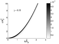
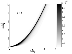
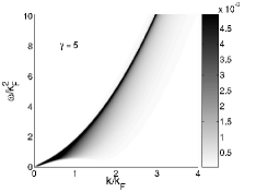
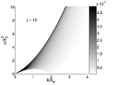
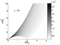
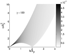
Figure 1: Density plots of the dynamical structure factor as a function of interaction. The horizontal axis is momentum (running up to $4k_{F}$), and the vertical axis represents energy transfer. Data obtained from systems of length $L=100$ with $N=100$ and $\gamma=0.25,1,5,10,20$ and $100$.

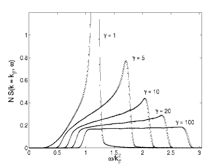
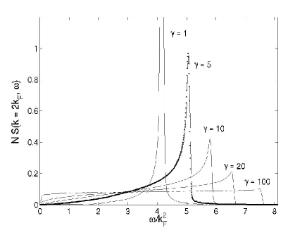
Figure 2: Fixed momentum plots of the dynamical structure factor for five representative values of the interaction parameter $\gamma$ obtained using $L=100$ and $N=100$ (continuous curves) and $L=80$ and $N=80$ (dots), such that $k_{F}=\pi$ in all cases. The energy $\delta$-function in equation (3) is a Gaussian of width $w=0.3$.

By inserting a summation over intermediate states, $S(k,\omega)$ is transformed into a sum of matrix elements of the density operator in the basis of Bethe eigenstates $|\alpha\rangle$,

$$S(k,\omega)=\frac{2\pi}{L}\sum_{\alpha}|\langle 0|\rho_{k}|\alpha\rangle|^{2}\delta(\omega-E_{\alpha}+E_{0})$$ (3)

where $\rho_{k}=\sum_{j=1}^{N}e^{-ikx_{j}}$. All of the elements in each term of this sum are fully determined by the Algebraic Bethe Ansatz, for a finite system with specified boundary conditions (we consider periodic systems in the present work). The Fock space is spanned by the set of Bethe wavefunctions, each fully determined by a set of $N$ rapidities $\{\lambda_{j}\}$, solution to the Bethe equations

$$\lambda_{j}+\frac{1}{L}\sum_{k}2\arctan\frac{\lambda_{j}-\lambda_{k}}{c}=\frac{2\pi}{L}I_{j}$$ (4)

in which $I_{j}$ are half-odd integers (integers) for even (odd) $N$. All solutions to these Bethe equations are real. Each set of distinct quantum numbers $\{I_{j}\}$, $I_{j}\neq I_{k}$ if $j\neq k$ defines a Bethe eigenstate participating in the sum (3). The energy and momentum of such a state are given by $E=\sum_{j}\lambda_{j}^{2}$ and $k=\sum_{j}\lambda_{j}=\frac{2\pi}{L}\sum_{j}I_{j}$. The ground-state itself is obtained from the set $\{I_{j}^{0}\}$, with $I_{j}^{0}=\frac{N+1}{2}-j$, $j=1,...,N$. The wavefunction of an eigenstate is given by the Bethe Ansatz, and its norm by the determinant of the Gaudin matrix GaudinBOOK ; KorepinCMP86 .

Matrix elements of the density operator in the basis of Bethe eigenstates were calculated with the Algebraic Bethe Ansatz in [SlavnovTMP79_82, ]. They are given by the determinant of a matrix whose entries are rational functions of the rapidities of the two eigenstates involved. For the sake of brevity we do not reproduce these expressions here.

What remains to be performed is the actual summation over intermediate states in (3). From this step onwards, everything is done numerically. The Fock space of intermediate states is scanned by navigating through choices of sets of quantum numbers. For each individual intermediate state, the Bethe equations are solved, and the matrix element is computed. To obtain smooth curves in energy, the energy delta function in (3) is broadened to a width equal to a multiple of the typical energy level spacing. The contribution to the dynamical structure factor sum is tallied until good convergence has been achieved. This is quantified by evaluating the $f$-sum rule,

$$\int\frac{d\omega}{2\pi}\omega S(k,\omega)=\frac{N}{L}k^{2}.$$ (5)

Since this is skewed towards high energy, and in view of the ordering of states in the scanning we perform (typically going from low-energy intermediate states to higher-energy ones), the saturation level of this sum rule represents a lower bound for the saturation of $S(k,\omega)$ itself.

Table 1: $f$-sum rule saturation percentage achieved at the two representative values of momentum used in Fig. 2. The method converges fastest in the strongly-interacting regime, the most difficult regime being intermediate interactions.

$\gamma$	0.25	1	5	10	20	100
$k_{F}$	99.52	99.44	99.48	99.45	99.80	99.97
$2k_{F}$	99.34	99.11	97.49	98.21	99.35	99.90

Table 2: Sound velocities for the interaction values considered here. A comparison is made between the finite-size value, and the infinite-size one.

$\gamma$	0.25	1	5	10	20	100
$v_{s}(N=100)$	0.9612	1.8350	3.5916	4.4818	5.2175	6.0395
$v_{s}(\infty)$	0.9594	1.8342	3.5912	4.4816	5.2173	6.0395

It is useful to recall here the nature of excitations in the Lieb-Liniger model, which come in two types LiebPR130 , Type I (“particles”) and Type II (“holes”) Exc . Type I are Bogoliubov-like quasiparticles that exist for any momentum, and represent states with one quantum number displaced outside the ground-state interval. Their dispersion relation is described in the thermodynamic limit by an integral equation, yielding a curve contained between the asymptotic limits $\epsilon_{I}(k)=k^{2}$ at $\gamma=0$ and $\epsilon_{I}(k)=k^{2}+2\pi n|k|$ for $\gamma\rightarrow\infty$. Type II excitations are holes in the ground-state distribution, and do not appear in Bogoliubov theory. They exist in the interval $|k|\leq k_{F}\equiv\pi n$, and their dispersion relation coincides with the lower threshold of the DSF. Low-energy Umklapp modes at $k=2k_{F}$ can be understood as excitations going from one side of the Fermi surface to the other. Both Type I and Type II dispersion relations approach $k\rightarrow 0$ with a slope equal to the velocity of sound $v_{s}(\gamma)$.

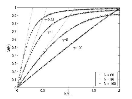
Figure 3: Static structure factor for four representative values of the interaction parameter $\gamma$. The three values of system size illustrate the smallness of finite-size effects. All curves saturate towards the limit $S(k\rightarrow\infty)=1$. The dashed lines are the small momentum asymptotic predictions $S(k)\simeq k/v_{s}$. Deviations in the $\gamma=5$ curve near $2k_{F}$ are commensurate with lack of saturation of the f-sum rule there (see Table I).

A remarkable feature in this method comes from the fact that it is not necessary to scan through the whole Fock space to get good saturation. Contributions from intermediate states with up to only a handful of particles are sufficient to achieve extremely good accuracy. The saturation of the $f$-sum rule (5) achieved for the $N=100$ curves in Fig. 2 is summarized in Table 1 (for lower values of $N$, even better saturation is achieved). Our algorithm is designed to recursively hunt for the most important terms in the multiparticle sum, in decreasing order of contribution to the DSF, and therefore to maximize the efficiency of the available numerical resources. Higher accuracy is obtained by using more computational time to include the contributions from more intermediate states.

Fig. 1 shows density plots for the DSF obtained with our method, for different values of $\gamma$. We used unit density $n=1$ with $L=100$ and $N=100$ (this compares with experimental particle numbers KinoshitaSCIENCE305 ; ParedesNATURE429 ). For small $\gamma$, the DSF is essentially a single delta peak centered on the Type I dispersion relation, $S(k,\omega)=\frac{Nk^{2}}{L\epsilon_{I}(k)}\delta(\omega-\epsilon_{I}(k))$. As $\gamma$ increases, the peak flattens but remains near the upper two-particle boundary. In particular, this confirms that the peak near the lower boundary observed in first-order RPA is an artefact of that method BrandPRA72_73 . Increasing $\gamma$ further towards the Tonks-Girardeau limit, the DSF approaches a constant over a finite frequency interval for a given momentum. All of this is illustrated more specifically for two specific values of momentum in Fig. 2. Fig. 3 shows $S(k)$, which qualitatively fits with quantum Monte Carlo results AstrakharchikPRA68 . At small momentum, we recover the prediction $S(k)\simeq k/v_{s}$ (see for example [AstrakharchikPRA70, ]). The curve for the largest interaction value, $\gamma=100$, also clearly approaches the well-known result $\lim_{\gamma\rightarrow\infty}S(k)=k/2k_{F}$ for $k\leq 2k_{F}$. Moreover, Fig. 1 shows that low-energy contributions near $2k_{F}$, which represent superfluidity-breaking Umklapp modes, are only important for large $\gamma$.

For all values of $\gamma$, the signal mostly lies between the two-particle continuum defined by convolution of the Type I and Type II dispersion relations. For general $k$, all the signal in fact lies strictly above the Type II dispersion relation modulo $2k_{F}$ translations, since there are no lower-energy states available. The upper two-particle bound is however not robust: multiparticle contributions give a nonzero signal at (in principle arbitrarily) large energy (coming from e.g. states with two or more particles of large but opposite momentum). In practice, however, the data shows that the onset of the DSF at finite $\gamma$ is followed by a sharp peak around the Type I dispersion, followed by a rapid decrease. We believe that in the thermodynamic limit, contributions from intermediate states with higher particle numbers smoothen the upper threshold into a high-frequency tail, as is the case for the corresponding correlators in quantum spin chains Pereira0603681 . The only exception is the Tonks-Girardeau limit, where both the lower and upper thresholds remain sharp.

To quantify finite-size effects in our results, we have included data for $N=80$ in Fig. 2 and for $N=60,80$ in Fig. 3 and given values for the effective $v_{s}(\gamma)$ (the conformal exponent $\eta$, such that $S(2k_{F},\omega)\simeq\omega^{\eta-2}$ at small $\omega$, is given by $\eta=4\pi n/v_{s}$) obtained for $N=100$ compared to the thermodynamic one in Table 2. Theoretical considerations based on Bethe Ansatz expressions for correlation functions KitanineNPB554 , similar to those used here, predict finite-size corrections of order $1/N$. The precise form of these $1/N$ corrections then depends on the specific boundary conditions used, but we believe that our results are close enough to the thermodynamic limit to make the choice of boundary conditions immaterial. Specifically, in Fig. 2, the only observable effect of increasing system size is a very slight shift of the main peaks of the DSF towards higher energy (for clarity we do not plot the $N=80$ results in the right-hand figure, but they show the same behaviour as in the left-hand one). The static structure factor plotted in Fig. 3 shows essentially no change for the different values of $N$ given. The variations observed fit comfortably within the deviation from perfection of the sum rule saturation achieved, which is the actual determining factor in the quality of our results. More important for theory is the question of a confining potential AstrakharchikPRA68 ; BatrouniPRA72 ; GattobigioJPB39 , which is present in experiments but breaks the integrability of the Lieb-Liniger model. We expect that experiments on large enough systems would on the other hand show correlations approaching those of a pure Lieb-Liniger model similar to those obtained here, or that experiments could be done in box-like geometries, where a variation of our method would be applicable.

Summarizing, we have computed the frequency- and momentum-dependent dynamical density-density correlation function of the one-dimensional interacting Bose gas (Lieb-Liniger model) for systems with finite numbers of particles, using a Bethe Ansatz-based numerical method. This goes beyond other available methods in offering a full characterization of the momentum and frequency dependence of the dynamical structure factor, provides a firm testing standard for other methods, and opens the way to many possible extensions (other correlators, systems with mixed statistics, finite temperatures) on which we will report in future publications.

J.-S. C. acknowledges useful discussions with N. A. Slavnov, M. J. Bhaseen, G. V. Shlyapnikov and J. T. M. Walraven. P. C. acknowledges discussions with M. Polini. This research was supported by the Stichting voor Fundamenteel Onderzoek der Materie (FOM) of the Netherlands.

References

- (1) L. Pitaevskii and S. Stringari, “Bose-Einstein Condensation”, Oxford, 2003.
- (2) D. S. Petrov, G. V. Shlyapnikov and J. T. M. Walraven, Phys. Rev. Lett. 85, 3745 (2000).
- (3) A. Görlitz et al., Phys. Rev. Lett. 87, 130402 (2001).
- (4) M. Greiner et al., Phys. Rev. Lett. 87, 160405 (2001).
- (5) H. Moritz et al., Phys. Rev. Lett. 91, 250402 (2003).
- (6) B. Paredes et al., Nature 429, 277 (2004).
- (7) T. Kinoshita, T. Wenger and D. S. Weiss, Science 305, 1125 (2004).
- (8) D. M. Gangardt and G. V. Shlyapnikov, Phys. Rev. Lett. 90, 010401 (2003); K. V. Kheruntsyan et al., Phys. Rev. A 71, 053615 (2005).
- (9) B. Laburthe Tolra et al., Phys. Rev. Lett. 92, 190401 (2004).
- (10) E. H. Lieb and W. Liniger, Phys. Rev. 130, 1605 (1963); E. H. Lieb, Phys. Rev. 130, 1616 (1963).
- (11) L. Tonks, Phys. Rev. 50, 955 (1936).
- (12) M. Girardeau, J. Math. Phys. (N.Y.) 1, 516 (1960).
- (13) C. N. Yang and C. P. Yang, J. Math. Phys. (N.Y.) 10, 1115 (1969).
- (14) F. Zambelli et al., Phys. Rev. A 61, 063608 (2000).
- (15) F. D. M. Haldane, Phys. Rev. Lett. 47, 1840 (1981).
- (16) A. Berkovich and G. Murthy, Phys. Lett. A 142, 121 (1989).
- (17) A. H. Castro Neto et al., Phys. Rev. B 50, 14032 (1994).
- (18) D. L. Luxat and A. Griffin, Phys. Rev. A 67, 043603 (2003).
- (19) M. Olshanii and V. Dunjko, Phys. Rev. Lett. 91, 090401 (2003).
- (20) J. Brand and A. Yu. Cherny, Phys. Rev. A 72, 033619 (2005); A. Yu. Cherny and J. Brand, Phys. Rev. A 73, 023612 (2006).
- (21) L. Pollet et al, Phys. Rev. Lett. 93, 210401 (2004).
- (22) G. E. Astrakharchik and S. Giorgini, Phys. Rev. A 68, 031602(R) (2003).
- (23) V. E. Korepin, N. M. Bogoliubov and A. G. Izergin, “Quantum Inverse Scattering Method and Correlation Functions”, Cambridge, 1993, and references therein.
- (24) V. E. Korepin, Commun. Math. Phys. 94, 93 (1984).
- (25) N. A. Slavnov, Teor. Mat. Fiz. 79, 232 (1989); ibid., 82, 389 (1990).
- (26) J.-S. Caux and J. M. Maillet, Phys. Rev. Lett. 95, 077201 (2005); J.-S. Caux, R. Hagemans and J. M. Maillet, J. Stat. Mech. (2005) P09003.
- (27) L.-M. Duan, Phys. Rev. Lett. 96, 103201 (2006).
- (28) J. Stenger et al., Phys. Rev. Lett. 82, 4569 (1999).
- (29) V. E. Korepin, Commun. Math. Phys. 86, 391 (1982).
- (30) M. Gaudin, “La fonction d’onde de Bethe”, Masson (Paris) (1983).
- (31) Although useful for visualizing low-energy excitations, this classification yields double counting (Type II particles are really a compound of low-momentum Type I particles LiebPR130 ). The Fock space itself is spanned by using only Type I.
- (32) G. E. Astrakharchik and L. Pitaevskii, Phys. Rev. A 70, 013608 (2004).
- (33) N. Kitanine, J. M. Maillet and V. Terras, Nucl. Phys. B554, 647 (1999).
- (34) R. G. Pereira et al., cond-mat/0603681.
- (35) G. G. Batrouni et al, Phys. Rev. A 72, 031602 (2005).
- (36) M. Gattobigio, J. Phys. B 39, S191 (2006).