Non-linear magneto-transport through small quantum dots at strong intra-dot correlations

Abstract

Nonlinear transport through a quantum dot is studied in the limit of weak and strong intra-dot Coulomb interaction. For the latter regime the nonequilibrium self-consistent mean field equations for energies and spectral weights of one-electron transitions are formulated. The increase of the bias-voltage window leads to a strong deviation from Gibbs statistics: the populations of states involved into a tunnelling are equalizing in this limit even at low temperature. For a symmetric coupling of a quantum dot to two leads we provide simple analytical relations between heights of the current steps and degeneracy of a spectrum in a two-dimensional parabolic dot in a perpendicular magnetic field in the both regimes.

I Introduction

Nowadays, quantum dots (QDs) are among common experimental tools to study properties of correlated electron systems at atomic scale, in a controllable manner. In particular, transport measurements through QDs provide a rich information on internal dynamics governed by external gate and bias voltages, and by the degree of coupling of the dot to the source and drain electrodes. Depending on the above conditions, a spectrum of a quantum dot, extracted from the single-electron spectroscopy, manifests a variety of features from shell structure to chaotic dynamics (see for review Refs.kou, ; RM, ).

One of the simplest quantum devices to study transport consists of two metallic contacts, attached via insulating/vacuum barriers to a QD. Combination of pieces with very different physical properties suggests that theoretical descriptions may require different approximations in accounting for the interactions in the constituents. In addition, the openings affects an intrinsic structure of initially closed quantum dot. Evidently, the energies of many-electron transitions (levels) acquire a width and both single- and many-particle processes contribute to the life-time of the levels. Moreover, the levels can be shifted due to the coupling of the QD to the leads. The shift can also be spin-sensitive due to many-electron nature of the electron transitions involved PRL .

For small QDs, when the size quantization of the carrier motion becomes important, and at low enough carrier density the strong electron correlations (SEC) affect the electron transport through the dot. At the weak dot-lead coupling and relatively small temperatures ($\lesssim 200$ mK), the intra-dot SEC are dominant in the tunnelling. At this (Coulomb blockade) regime, the charging energy $E_{C}$, that needed to add an electron to the dot with N electrons, considerably exceeds the level spacing and the thermal energy $k_{B}T$. According to the classical Coulomb blockade picture, the transport is only allowed when the N and (N+1) states are both energetically accessible (cf Ref.tr, ). The conductance usually shows a Breit-Wigner resonance as a function of gate voltage indicating that electrons pass by a discrete level in the quantum dot by a resonant tunnelling. At lower temperature the co-tunnelling events predicted in Ref.Av, become visible; they involve the simultaneous tunnelling of two or more electrons over virtual states, giving rise to the current inside the Coulomb diamond Fran . With a further decrease of the temperature, Kondo-type effects can develop if the system has quasi-degenerate localized states. For example, a weak current through QD, observed within the Coulomb blockade regime KondoEff , is interpreted as a Kondo effect (see for a review Ref.PG, ).

Recently, in experiments with a small quantum dot in the Coulomb-blockade regime ihn , a fine structure was observed in the conductance as a function of gate voltage versus source-drain voltage. It was suggested that this phenomenon is mainly due to a co-tunnelling Av . The theory of co-tunnelling Av neglects, however, specific quantum effects caused by a strong Coulomb interaction (SCI), which affect the transition energies and the tunnelling rates. On the other hand, numerous papers devoted to quantum effects in transport through QDs are focused on the analysis of Kondo phenomenon in single-level QD models (cf Refs.Kondo, ) in a linear-response regime, which is well understood nowadays. However, the single-electron spectroscopy clearly indicates that a shell structure of small dots plays an essential role in the transport and weak dot-lead coupling tr when the temperature is still low, but above the Kondo temperature. This becomes especially evident, when the confining energy exceeds the charging energy ota (hereafter, this regime is called a weak Coulomb interaction (WCI) regime). One of our goals is to present a self-consistent approach for a nonlinear transport through a multilevel quantum dot in the SCI regime. We will demonstrate that even in this regime a shell structure of a small dot can be extracted from the analysis of nonlinear current as a function of a finite bias voltage. We will show also that the conductance inside of the ”Coulomb diamond” is governed by spectral weights of one-electron transitions, that complement the co-tunnelling picture.

In this paper we consider the transport through a small QD with a parabolic effective confining potential. As an input, we use the intrinsic structure of a closed dot. The use of the parabolic confinement is well justified by experimental observations, for example, magic numbers of a two-dimensional harmonic oscillator tar and a fulfilment of the Kohn theorem Kohn in far-infrared spectroscopy experiments SM . The eigen problem of interacting electrons in a closed parabolic QD can be solved approximately within an unrestricted Hartree-Fock approximation (cf Ref.pl03, ) or local density approximation to a density functional theory RM . When the confinement dominates the Coulomb interaction, the eigen spectrum is well approximated by the Fock-Darwin levels fock . Recent experiments nicely confirm this fact, indeed (see, for example, experimental results in Ref.ota, ). This allows to describe a QD within a single-particle picture of electrons in an effective parabolic potential (hereafter we denote such states as $|\gamma\rangle$ ). We consider the SCI regime in the limit of very strong intra-dot interaction (”Hubbard” $U\rightarrow\infty$). In this case the Hamiltonian of QD at the SCI regime is diagonalized by the states $\left|0\right\rangle$ and $\left|\gamma\right\rangle$, and only the transitions between empty and single-electron occupied QD states contribute into transport. The assumption that the states $\left|0\right\rangle$ and $\left|\gamma\right\rangle$ are well separated by a large energy gap from two- , three-, etc correlated states can be easily verified, for example, within an analytical model for two-electron parabolic quantum dot din . At zero coupling to leads one-electron energies coincide in both the WCI and SCI regimes. It presents a nice opportunity to study in a transparent way the role of the Coulomb interaction within this particular charge sector. Although the bare energies of QDs coinside n these two regimes, in the SCI limit a hopping of an electron into a QD is determined by the occupation numbers of the QD states. We employ here the Hubbard operator technique ig which is specially designed for such cases. The mean field theory in terms of the Hubbard operators is quite different from the one constructed for the WCI regime. For example, the consideration of a single spin flip in the infinite $U$ Hubbard model shows that the mean field theory of this type gives the same results with both Gutzwiller wave function and the three-body Faddeev equations in this limit RuckSchmR .

As pointed out above, we will analyze the transport through QD in non-linear with respect to the bias voltage regime at the weak dot-lead coupling. In other words, the transparency of junctions is assumed to be small. The latter requirement has a pragmatic basis as well: enormous efforts for a fabrication of QDs are motivated by the desire to understand the inner structure and to exploit it in various applications.

Thus, the coupling to the leads will be treated perturbatively. Below we focus on the transport in the resonant-tunnelling regime, where the Kondo physics is not involved. In the language of the Anderson impurity theory, we will be interested in the intermediate-valence regime, when QD levels are located within the range of the resonant tunnelling. We recall that in this region such a widely used method as a mean-field approximation in slave-boson theory geor is not applicable, in contrast to our approach.

The paper is organized as follows: in Section II we will discuss our model Hamiltonian, the nonlinear current in terms of the Hubbard operators and formulate the mean field approximation. Section III is devoted to the derivation of equations for population numbers and energy shifts in the diagonal approximation. The results for the transport through a parabolic quantum dot in a perpendicular magnetic field at weak (WCI) and strong (SCI) intra-dot Coulomb interaction are given in Section IV. The conclusions are finally drawn in Section V. Two Appendices contain some technical details. Some preliminary results of our analysis are presented in Ref.JPhysC,

II Formalism

II.1 Model Hamiltonian and current

As discussed in the Introduction, we consider the system which is decribed by the following Hamiltonian

$$H=H_{l}+H_{r}+H_{QD}+H_{t},$$ (1)

where

$$H_{\lambda}=\sum_{k\sigma\in\lambda}\varepsilon_{\lambda k\sigma}\,c_{\lambda k\sigma}^{\dagger}c_{\lambda k\sigma}$$

$$H_{QD}=\sum_{\gamma}\varepsilon_{\gamma}n_{\gamma}+\sum_{\gamma\neq\gamma^{\prime}}U_{\gamma\gamma^{\prime}}n_{\gamma}n_{\gamma^{\prime}},\quad n_{\gamma}=d_{\gamma}^{\dagger}d_{\gamma}$$

$$H_{t}=\sum_{k\sigma\in\lambda,\lambda,\gamma}\left(v_{k\sigma,0\gamma}^{\lambda}\,c_{\lambda k\sigma}^{\dagger}d_{\gamma}+h.c.\right)$$

The term $H_{\lambda}$ describes noninteracting electrons with the energy $\varepsilon_{\lambda k\sigma}$, wave number $k$ and spin $\sigma$ in the lead $\lambda=l,r$. The closed dot is modelled by $H_{QD}$. Here $\varepsilon_{\gamma}$ is the energy of electron with a set of single-electron quantum numbers $\gamma$ in the confining potential of the closed QD at $U=0$. Tunnelling between the dot and leads is described by the term $H_{t}$; the matrix elements $v_{k\sigma,0\gamma}^{\lambda}$ here couple the left and the right contacts with a QD. The ratio of level spacing of noninteracting electrons in a QD to ”Hubbard $U$”, $\left|\varepsilon_{\gamma}-\varepsilon_{\gamma^{\prime}}\right|/U=\delta\varepsilon_{\gamma\gamma^{\prime}}/U$ determines whether the intra-dot electrons are in the regime of weak ($\delta\varepsilon_{\gamma\gamma^{\prime}}/U>1$) or strong ($\delta\varepsilon_{\gamma\gamma^{\prime}}/U<1$) Coulomb interaction.

The Hamiltonian of QD is transformed into a diagonal form by introducing the Hubbard operators hub (see also Appendix A). As a result, the Hamiltonian (1) acquires the form:

$$H=\sum_{k\sigma\lambda}\varepsilon_{\lambda k\sigma}c_{\lambda k\sigma}^{\dagger}c_{\lambda k\sigma}+\varepsilon_{0}Z^{00}+\sum_{\gamma}\varepsilon_{\gamma}Z^{\gamma\gamma}$$

$$+\sum_{k\sigma\lambda,\gamma}\left(v_{k\sigma,\gamma}^{\lambda}c_{\lambda k\sigma}^{\dagger}X^{0\gamma}+h.c.\right)$$ (2)

Following Ref.MW, , we obtain (see Appendix B) for the ”left” steady current

$$J_{l} = \frac{ie}{\hbar}\sum_{\gamma\gamma^{\prime}}\int d\omega\Bigg{\{}\left[\Gamma_{\gamma^{\prime}\gamma}^{l}(\omega)-\Gamma_{\gamma^{\prime}\gamma}^{r}(\omega)\right]G_{\gamma,\gamma^{\prime}}^{<}(\omega)$$ (3)

$$+ \left[\Gamma_{\gamma^{\prime}\gamma}^{l}(\omega)f_{l}(\omega)-\Gamma_{\gamma^{\prime}\gamma}^{r}(\omega)f_{r}(\omega)\right]\times$$

$$\times\left[G_{\gamma,\gamma^{\prime}}^{R}(\omega)-G_{\gamma,\gamma^{\prime}}^{A}(\omega)\right]\Bigg{\}}$$

The current (3) is expressed in terms of Green functions (GFs) defined for the Hubbard operators :

$$G_{\gamma,\gamma^{\prime}}^{\eta}(\omega)=\int d(t-t^{\prime})e^{i\omega(t-t^{\prime})}G_{\gamma,\gamma^{\prime}}^{\eta}(t,t^{\prime}),\;\eta=<,>,R,A$$

$$G_{\gamma,\gamma^{\prime}}^{<}(t,t^{\prime})\equiv i\left\langle X^{\gamma^{\prime}0}(t^{\prime})X^{0\gamma}(t)\right\rangle$$

$$G_{\gamma,\gamma^{\prime}}^{>}(t,t^{\prime})\equiv-i\left\langle X^{0\gamma}(t)X^{\gamma^{\prime}0}(t^{\prime})\right\rangle$$

$$G_{\gamma,\gamma^{\prime}}^{R/A}(t,t^{\prime})\equiv\mp i\theta(\pm t\mp t^{\prime})\left\langle\left\{X^{0\gamma}(t),X^{\gamma^{\prime}0}(t^{\prime})\right\}\right\rangle$$ (4)

The GFs depend on difference of times (or one frequency $\omega$) because we consider the steady states only. Note that for a wide conduction band, i.e., when the bandwidth is much larger than any other parameter in the problem, the width function

$$\Gamma_{\gamma\gamma^{\prime}}^{\lambda}(\omega)=\pi\sum_{\,k\sigma}v_{\gamma^{\prime},k\sigma}^{\lambda}\delta(\omega-\varepsilon_{\lambda k\sigma})v_{k\sigma,\gamma}^{\lambda}$$ (5)

weakly depends on $\omega$ and will be replaced by a constant when we will consider a particular model (see also Appendices A,B)

Thus, we have to find the GFs $G_{\gamma,\gamma^{\prime}}^{\eta}$. As well-known, the Dyson equation does not exist for any many-electron GF (particularly, for the GF defined on the Hubbard operators), since the (anti)commutation of many-electron operators (see Eq.(A.12)) generates not a ”c”-number as in case of fermions or bosons, but an operator again. The perturbation theory for the many-electron GFs reflects this fact by generating the additional graphs compared to the conventional theory for fermions or bosons (examples are given in Ref.ig, ; also see a Sec.IIb). Therefore, those of results of Refs.MW, ; JWM, , which are derived on the basis of a Dyson equation for the retarded and advanced GFs, should be re-inspected. As will be seen below, the formulas analogous to the ones derived in Refs.MW, ; JWM, are valid only within the  well-known Hubbard-I approximation and mean-field approximations (MFA) ig (Ref.ig, will be referred below as I). The same approximation is sufficient for calculation of the transport properties at small transparencies of the junctions too.

Let us introduce the full width $\Gamma$ and dimensionless partial widths $\alpha$:

$$\Gamma_{\gamma^{\prime}\gamma}=\Gamma_{\gamma^{\prime}\gamma}^{l}+\Gamma_{\gamma^{\prime}\gamma}^{r},\quad\alpha_{\gamma^{\prime}\gamma}^{\lambda}=\Gamma_{\gamma^{\prime}\gamma}^{\lambda}/\Gamma_{\gamma^{\prime}\gamma},$$ (6)

When the coupling to leads is so small that the widths $\Gamma$ of the transitions are much smaller than the temperature $T$, $\beta\Gamma\ll 1$ (where $\beta=1/T$) and the level spacing, $\Gamma/\delta\epsilon_{\gamma\gamma^{\prime}}\ll 1$, the mixing of levels due to non-diagonal terms does not influence the physics of transport. Namely this range of parameters is exploited usually in experiments and will be in the scope of our interests (starting from Sec.III). Neglecting the non-diagonal terms leads to the diagonal approximation, where $\Gamma_{\gamma^{\prime}\gamma}=\delta_{\gamma^{\prime}\gamma}\Gamma_{\gamma}$, $\alpha_{\gamma\gamma^{\prime}}^{\lambda}=\delta_{\gamma^{\prime}\gamma}\alpha_{\gamma}^{\lambda}$. The expression for the current becomes:

$$J = \frac{ie}{\hbar}\sum_{\gamma}\Gamma_{\gamma\gamma}\int d\omega\Bigg{\{}\left[\alpha_{\gamma}^{l}-\alpha_{\gamma}^{r}\right]G_{\gamma,\gamma}^{<}(\omega)$$ (7)

$$+ \left[\alpha_{\gamma}^{l}f_{l}(\omega)-\alpha_{\gamma}^{r}f_{r}(\omega)\right]\left[G_{\gamma,\gamma}^{R}(\omega)-G_{\gamma,\gamma}^{A}(\omega)\right]\Bigg{\}}$$

The advantage of the Wingreen and Meir formulation MW lies in the fact that the current (in our case Eq.(3)) is expressed in terms of the GFs of a QD only. We recall that this result can be obtained only for non-interacting conduction electrons. Thus, our next-step goal is to derive equations for GFs $G_{\gamma,p^{\prime}0}^{<,R,A}$ in the MFA.

II.2 Exact equations on imaginary-time axis

Our derivation is based on the approach PRL ; ig that employs the ideas suggested by Schwinger schwinger and developed further by Kadanoff and Baym KB . Since we consider only the intra-dot Coulomb interaction, the conduction-electron subsystems are linear and can be integrated  out. Instead an additional effective interactions between electrons in a QD arises. Following Ref.KB, , equations for the QD subsystem will be written in terms of functional derivatives with respect to external auxiliary sources. The derivation of the equations will be performed in three steps. Firstly, we derive exact equations for the QD GFs on the imaginary-time axis. Secondly, the MFA will be formulated. Thirdly, we will perform a continuation of these equations onto the real-time axis.

The time evolution of the Hubbard operator $X^{0\gamma}$ is defined by the commutator

$$[X^{0\gamma},H] = \Delta_{\gamma 0}^{(0)}X^{0\gamma}+$$

$$+ \sum_{k\sigma\in\lambda,\lambda,\gamma_{1}\neq\gamma}\,v_{\gamma_{1},k\sigma}^{\lambda}\left(\delta_{\gamma_{1}\gamma}Z^{00}+Z^{\gamma_{1}\gamma}\right)c_{\lambda k\sigma},$$

which contains non-linear terms. These terms produce GFs of the type $-i\langle T\left(\delta_{\gamma^{\prime}\gamma}Z^{00}(t)+Z^{\gamma^{\prime}\gamma}(t)\right)c_{\lambda k^{\prime\prime}\sigma}(t)c_{\lambda k^{\prime}\sigma}^{\dagger}(t^{\prime})\rangle$. Below we omit the summation signs: summation over repeating indices is implied unless otherwise stated.

To proceed further, we introduce the auxiliary sources $U^{00}(t),U^{\gamma\gamma^{\prime}}(t)$ into a definition of the GFs:

$$G_{AB}(t,t^{\prime})=\frac{1}{i}\left\langle TA(t)B(t^{\prime})\right\rangle_{U}=\frac{1}{i}\frac{\left\langle TA(t)B(t^{\prime})S(t_{0},\beta)\right\rangle}{\left\langle TS(t_{0},\beta)\right\rangle},$$

$$S(t_{0},\beta)\equiv T\exp\Bigg{\{}-i\int_{t_{0}}^{t_{0}-i\beta}dt_{1}\Bigg{[}U^{00}(t_{1})Z^{00}(t_{1})+$$

$$+\sum_{\gamma\gamma^{\prime}}U^{\gamma\gamma^{\prime}}(t_{1})Z^{\gamma\gamma^{\prime}}(t_{1})\Bigg{]}\Bigg{\}}.$$ (9)

Here $A,B=c_{\lambda k\sigma},X^{0\gamma}$; ($\lambda=l,$) for for the left and ($\lambda=r$) for the right contacts. We will use the following notations:

$$\left(\begin{array}[c]{cc}C_{k\sigma,k^{\prime}\sigma^{\prime}}(t,t^{\prime})&G_{k\sigma,\gamma^{\prime}}(t,t^{\prime})\\ G_{\gamma,k^{\prime}\sigma^{\prime}}(t,t^{\prime})&G_{\gamma,\gamma^{\prime}}(t,t^{\prime})\end{array}\right)=\frac{1}{i}\left(\begin{array}[c]{cc}\left\langle Tc_{\lambda k\sigma}(t)c_{\lambda^{\prime}k^{\prime}\sigma^{\prime}}^{\dagger}(t^{\prime})\right\rangle_{U}&\left\langle Tc_{\lambda k\sigma}(t)X^{\gamma^{\prime}0}(t^{\prime})\right\rangle_{U}\\ \left\langle TX^{0\gamma}(t)c_{\lambda^{\prime}k^{\prime}\sigma^{\prime}}^{\dagger}(t^{\prime})\right\rangle_{U}&\left\langle TX^{0\gamma}(t)X^{\gamma^{\prime}0}(t^{\prime})\right\rangle_{U}\end{array}\right).$$ (10)

The equation of motion for the GFs $C_{k\sigma,k^{\prime}\sigma^{\prime}}(t,t^{\prime})$ and $G_{k\sigma,\gamma^{\prime}}(t,t^{\prime})$ are simple:

$$\left(i\partial_{t}-\varepsilon_{\lambda k\sigma}\right)C_{k\sigma,k^{\prime}\sigma^{\prime}}(t,t^{\prime})=\delta_{kk^{\prime}}\delta_{\sigma\sigma^{\prime}}+$$

$$+\sum_{\gamma^{\prime\prime}}\,v_{k\sigma,\gamma^{\prime\prime}}^{\lambda}G_{\gamma^{\prime\prime},k^{\prime}\sigma^{\prime}}(t,t^{\prime})$$ (11)

$$\left(i\partial_{t}-\varepsilon_{\lambda k\sigma}\right)G_{k\sigma,\gamma^{\prime}}(t,t^{\prime})=\sum_{\gamma^{\prime\prime}}\,v_{k\sigma,\gamma^{\prime\prime}}^{\lambda}G_{\gamma^{\prime\prime},\gamma^{\prime}}(t,t^{\prime})$$

(12)

As seen from Eq.(11), a zero GF $C_{k\sigma,k^{\prime}\sigma^{\prime}}^{(0)}$ satisfies the equation

$$\int dt_{1}\sum_{k^{\prime\prime}}\{[i\partial_{t}-\varepsilon_{\lambda k\sigma}]\delta(t-t_{1})\}C_{k\sigma,k^{\prime}\sigma^{\prime}}^{(0)}(t,t^{\prime}) \equiv$$ (13)

$$\delta_{kk^{\prime}}\delta_{\sigma\sigma^{\prime}}\delta(t-t^{\prime})$$

Hereafter the integrals are taken between $t_{0}$ and $t_{0}-i\beta$, if the other limits are not specified explicitly; here $t_{0}$ is an arbitrary moment. With the aid of this equation, Eqs.(11),(12) can be cast in the form of integral equations:

$$C_{k\sigma,k^{\prime}\sigma^{\prime}}(t,t^{\prime}) = C_{k\sigma}^{(0)}(t,t^{\prime})\delta_{kk^{\prime}}\delta_{\sigma\sigma^{\prime}}+$$

$$+ \sum_{\gamma^{\prime\prime}}\int dt_{1}C_{k\sigma}^{(0)}(t,t_{1})v_{k\sigma,\gamma^{\prime\prime}}^{\lambda}G_{\gamma^{\prime\prime},k^{\prime}\sigma^{\prime}}(t_{1},t^{\prime})$$

$$G_{k\sigma,\gamma^{\prime}}(t,t^{\prime}) = \sum_{\gamma_{2}}\,\int dt_{1}C_{k\sigma}^{(0)}(t,t_{1})v_{k\sigma,\gamma_{2}}^{\lambda}G_{\gamma_{2},\gamma^{\prime}}(t_{1},t^{\prime})$$

Analogously, using the equation for the GF $G_{\gamma^{\prime\prime},k^{\prime}\sigma^{\prime}}(t_{1},t^{\prime})$ with respect to the right time $t^{\prime}$, we obtain

$$G_{\gamma^{\prime\prime},k^{\prime}\sigma^{\prime}}(t,t^{\prime})=\sum_{\gamma_{1}}\,\int dt_{1}G_{\gamma^{\prime\prime},\gamma_{1}}(t,t_{1})v_{\gamma_{1},k^{\prime}\sigma^{\prime}}^{\lambda}C_{k^{\prime}\sigma^{\prime}}^{(0)}(t_{1},t^{\prime})$$ (16)

The equation for $G_{\gamma,\gamma^{\prime}}(t,t^{\prime})=-i\left\langle TX^{0\gamma}(t)X^{\gamma^{\prime}0}(t^{\prime})\right\rangle_{U}$ has, however, more complex form:

$$\left[\delta_{\gamma^{\prime}\gamma}i\partial_{t}-\Delta_{\gamma\gamma_{1}}^{(0)}(t)\right]G_{\gamma_{1},\gamma^{\prime}}(t,t^{\prime})=\delta(t-t^{\prime})P^{\gamma\gamma^{\prime}}(t)+$$

$$\sum_{k\sigma\in\lambda,\lambda,\gamma_{1}}\,v_{\gamma_{1},k\sigma}^{\lambda}\frac{1}{i}\left\langle T\left(\delta_{\gamma_{1}\gamma}Z^{00}+Z^{\gamma_{1}\gamma}\right)c_{\lambda k\sigma}(t)X^{\gamma^{\prime}0}(t^{\prime})\right\rangle_{U},$$

(17)

where

$$P^{\gamma\gamma^{\prime}}(t)\equiv\left\langle T\left\{X^{0\gamma}(t),X^{\gamma^{\prime}0}(t)\right\}\right\rangle_{U}$$ (18)

$$\Delta_{\gamma\gamma_{1}}^{(0)}(t)=\Delta_{\gamma}^{(0)}\delta_{\gamma_{1}\gamma}+\left[U^{\gamma\gamma_{1}}(t)-\delta_{\gamma_{1}\gamma}U^{00}(t)\right]$$

Here $\Delta_{\gamma}^{(0)}\equiv\varepsilon_{\gamma}-\varepsilon_{0}$ is the transition energy between the single-electron state and the one without electrons in a QD. We choose $\varepsilon_{0}=0$. The term $\left(U^{\gamma\gamma^{\prime}}(t)-\delta_{\gamma^{\prime}\gamma}U^{00}(t)\right)$ is due to the differentiation of $S(t_{0},\beta)$ (cf Ref.KB, ).

Below, we will proceed under the standard assumption that the interaction is absent at infinitely remote time $t_{0}\rightarrow-\infty$ and is switched on adiabatically. This assumption does not affect our approach, since we study a stationary regime. In this case we use the relation:

$$\langle TZ^{\xi}(t)X^{0\gamma}(t)B(t^{\prime})\rangle_{U}=$$

$$\left(\langle TZ^{\xi}(t)\rangle+i\frac{\delta}{\delta U^{\xi}(t)}\right)\langle TX^{0\gamma}(t)B(t^{\prime})\rangle_{U}$$ (19)

that follows from a functional derivative $\delta/\delta U^{\xi}(t)$ of Eq.(9) (here $\xi=[00],[\gamma\gamma^{\prime}]$).

With the aid of Eq.(19), using Eq.(LABEL:G_cXint) and the definition for the effective interaction via conduction electrons

$$V_{\gamma_{1}\gamma_{2}}(t,t_{1})=\sum_{k\sigma\in\lambda,\lambda}v_{\gamma_{1},k\sigma}^{\lambda}C_{k\sigma}^{(0)}(t,t_{1})v_{k\sigma,\gamma_{2}}^{\lambda}$$ (20)

(see also Eq.(B.7)), we transform Eq.(17) to the form

$$\left[\delta_{\gamma\gamma_{1}}i\partial_{t}-\Delta_{\gamma\gamma_{1}}^{(0)}(t)\right]G_{\gamma_{1},\gamma^{\prime}}(t,t^{\prime})=\delta(t-t^{\prime})P^{\gamma\gamma^{\prime}}(t)$$

$$+\sum_{\gamma_{2}\gamma_{1}}\,\int dt_{1}V_{\gamma_{1}\gamma_{2}}(t,t_{1})\Bigg{(}P^{\gamma\gamma_{1}}(t)+i\delta_{\gamma\gamma_{1}}\frac{\delta}{\delta U^{00}(t)}+$$

$$+i\frac{\delta}{\delta U^{\gamma_{1}\gamma}(t)}\Bigg{)}G_{\gamma_{2},\gamma^{\prime}}(t_{1},t^{\prime})$$ (21)

Here, we used also that $\delta C_{k\sigma}^{(0)}/\delta U=0$.

Eq.(21) is the exact equation for the GF $G_{\gamma,\gamma^{\prime}}(t,t^{\prime})$ on the imaginary time axis. Since all other GFs are expressed in terms of the $G_{\gamma^{\prime\prime},\gamma}$, the iteration of Eq.(21) with respect to the effective interaction generates a full perturbation theory. However, within this formulation of the theory, the continuation from the imaginary time axis to the real one should be performed in each term of the expansion.

The well-known ”Hubbard-I” (HI) approximation can be obtained from Eq.(21) by putting therein $\delta G_{\gamma^{\prime\prime},\gamma}/\delta U=0$. Let us define a zero locator $D_{\gamma,\gamma^{\prime}}^{(0)}(t,t^{\prime})$

$$\int dt_{1}\left\{\left[\delta_{\gamma\gamma_{1}}i\partial_{t}-\Delta_{\gamma\gamma_{1}}^{(0)}(t)\right]\delta(t-t_{1})\right\}D_{\gamma_{1},\gamma_{2}}^{(0)}(t_{1},t^{\prime})$$

$$\equiv\int dt_{1}\left[D^{(0)-1}(t,t_{1})\right]_{\gamma,\gamma_{1}}D_{\gamma_{1},\gamma_{2}}^{(0)}(t_{1},t^{\prime})$$

$$=\delta(t-t^{\prime})\delta_{\gamma\gamma_{2}}$$ (22)

In the HI approximation, the locator is defined by a solution to the equation:

$$\int dt_{1}\sum_{\gamma_{1}}\Bigg{\{}\left[\delta_{\gamma\gamma_{1}}i\partial_{t}-\Delta_{\gamma\gamma_{1}}^{(0)}(t)\right]\delta(t-t_{1})-$$

$$S_{\gamma,\gamma_{1}}^{HI}(t,t_{1})\Bigg{\}}D_{\gamma_{1},\gamma_{3}}^{HI}(t_{1},t^{\prime})=\delta_{\gamma\gamma_{3}}\delta(t-t^{\prime}),$$ (23)

where

$$S_{\gamma,\gamma_{1}}^{HI}(t,t_{1})=\sum_{\gamma_{2}}P^{\gamma\gamma_{2}}(t)\,V_{\gamma_{2}\gamma_{1}}(t,t_{1})$$ (24)

Using the above equations, we rewrite Eq.(21) in the form

$$\int dt_{1}\sum_{\gamma_{1}}\Bigg{\{}\left[D^{HI,-1}(t_{1},t^{\prime})\right]_{\gamma,\gamma_{1}}-$$ (25)

$$-\tilde{S}_{\gamma,\gamma_{1}}(t,t_{1})\Bigg{\}}G_{\gamma_{1},\gamma^{\prime}}(t_{1},t^{\prime})=\delta(t-t^{\prime})P^{\gamma\gamma^{\prime}}(t^{\prime})$$

with

$$\int dt_{1}\sum_{\gamma_{1}}\tilde{S}_{\gamma,\gamma_{1}}(t,t_{1})G_{\gamma_{1},\gamma^{\prime}}(t_{1},t^{\prime})\equiv$$ (26)

$$i\sum_{\gamma_{2}\gamma_{1}}\,\int dt_{1}V_{\gamma_{1}\gamma_{2}}(t,t_{1})\left(\delta_{\gamma\gamma_{1}}\frac{\delta G_{\gamma_{2},\gamma^{\prime}}(t_{1},t^{\prime})}{\delta U^{00}(t)}+\frac{\delta G_{\gamma_{2},\gamma^{\prime}}(t_{1},t^{\prime})}{\delta U^{\gamma_{1}\gamma}(t)}\right)$$

One may notice that Eq.(26) has a simple form in symbolic notations

$$D_{HI}^{-1}G+V\frac{\delta G}{\delta U}=P$$ (27)

This equation suggests that the full locator $D$ can be defined by the equation

$$\sum_{\gamma_{1}}\int dt_{1}[D(t,t_{1})]_{\gamma,\gamma_{1}}^{-1}G_{\gamma_{1},\gamma^{\prime}}(t_{1},t^{\prime})=\delta(t-t^{\prime})P^{\gamma\gamma^{\prime}}(t^{\prime}),$$ (28)

where

$$[D(t,t_{1})]_{\gamma,\gamma_{1}}^{-1}\equiv[D^{0}(t,t_{1})]_{\gamma,\gamma_{1}}^{-1}-S_{\gamma,\gamma_{1}}(t,t_{1})]$$

and the full self-operator is defined as

$$S_{\gamma,\gamma_{1}}=S_{\gamma,\gamma_{1}}^{HI}+\tilde{S}_{\gamma,\gamma_{1}}$$ (29)

The magnitude $S_{\gamma,\gamma_{1}}$ has been named in I as ”a self-operator” in order to distinguish it from the standard self-energy operator. In fact, the magnitude $\tilde{S}_{\gamma,\gamma_{1}}(t,t^{\prime})\,$ renormalizes the transition energies in a QD as well as the end-factors $P^{\gamma\gamma^{\prime}}(t)$. Indeed, one can see from Eq.(28) that

$$G_{\gamma_{1},\gamma^{\prime}}(t,t^{\prime})=D_{\gamma_{1},\gamma_{2}}(t,t^{\prime})P^{\gamma_{2}\gamma^{\prime}}(t^{\prime})$$ (30)

and, therefore, $P^{\gamma_{2}\gamma^{\prime}}(t^{\prime})$ enters into the equations for the GFs under the sign of the functional derivative. Being an expectation value from the anticommutator of many-electron operators, it is not a constant (like in the cases of Bose- or Fermi-operators). Therefore, its functional derivative is nonzero and generates a sub-set of graphs that do not appear in standard techniques for fermions and bosons. These graphs describe kinematic interactions.

II.3 The energy shifts (imaginary time).

An effective interaction of the intra-dot states via conduction electrons arises in both the WCI and SCI regimes. In both cases the lowest orders of perturbation theory contains the terms with integration over wide energy region of the continuous spectrum and, therefore, it results in finite widths of the intra-dot states. Particularly, in the SCI regime the width is provided already by the Hubbard-I approximation. Below we will show that in contrast to the WCI regime, in the SCI case the width depends on the population of the many-electron states which are involved into single-electron transition in question. This fact is more or less trivial consequence of non-Fermi/Bose commutation relations between Hubbard operators. A non-trivial consequence of it is kinematic interaction that shift transitions energies $\Delta_{\gamma}^{(0)}$ in a QD. The correlation-caused shift arises in a natural way within the mean-field approximation in slave-boson theory (see, e.g., Ref.langreth ). This approach misses, however, the spin and orbital sensitivity of the shifts for different levels. This obstacle can be resolved by means of the Hubbard operators formalism (cf I and Ref.PRL, ). In the present paper we use also the mean field approximation, which is similar in spirit to the one of Ref.langreth, . The details and physical meaning of our MFA, however, are different.

The MFA for the Hubbard operator GFs have been defined in I on the imaginary-time axis by two conditions: first, the dynamical scattering on Bose-like excitations is neglected, i.e., $\delta P/\delta U=0$ and, second, full vertex $\Gamma\equiv\delta D^{-1}/\delta U\$ is replaced by zero one, $\Gamma_{0}\equiv\delta D_{0}^{-1}/\delta U$. In other words, the MFA omits the fluctuations around the stationary solutions. The advantage of formulation of the theory in terms of Hubbard operators compared the slave-boson technique consists in the following. The MFA can be derived for a general case of an arbitrary Hubbard-operator algebra, or, in physical terms, for the case of arbitrary number and a type of (Bose- or Fermi-like) transitions (see I). Besides, one can go beyond the MFA in a systematic way. For example, in the presence of the long-range part of the Coulomb interaction one can reformulate theory in terms of screened interaction (see Ref.condmatII ).

In order to develop the MFA we have to extract from the self-operator $\tilde{S}$ the local-in-time contribution in the lowest order with respect to the effective interaction $V$. The self-operator $\tilde{S}$ (see Eq.(26)) is already proportional to the interaction $V_{\gamma\gamma^{\prime}}$. Therefore, one should calculate only the derivative $\delta G/\delta U$ in the lowest order with respect to the interaction. We recall that the interaction $V_{\gamma^{\prime}\gamma}(t,t_{1})$ does not depend on $U^{\xi}$. Thus, the derivative is

$$\frac{\delta G_{\gamma_{2},\gamma^{\prime}}(t_{1},t_{2})}{\delta U^{\xi}(t)}=\frac{\delta\left[D_{\gamma_{2},\gamma_{5}}(t_{1},t_{2})P^{\gamma_{5}\gamma^{\prime}}(t_{2})\right]}{\delta U^{\xi}(t)}$$ (31)

$$=\frac{\delta D_{\gamma_{2},\gamma_{5}}(t_{1},t_{2})}{\delta U^{\xi}(t)}P^{\gamma_{5}\gamma^{\prime}}(t_{2})+D_{\gamma_{2},\gamma_{5}}(t_{1},t_{2})\frac{\delta P^{\gamma_{5}\gamma^{\prime}}(t_{2})}{\delta U^{\xi}(t)}$$

The second term in Eq.(31) expresses the dynamical re-scattering process

$$\delta P^{\gamma_{5},\gamma^{\prime}}/\delta U^{\xi}\propto\left\langle TZ^{00}Z^{\xi}\right\rangle-$$

$$-\left\langle TZ^{00}\right\rangle\left\langle TZ^{\xi}\right\rangle+\left\langle TZ^{\gamma_{4}\gamma_{5}}Z^{\xi}\right\rangle-\left\langle TZ^{\gamma_{4}\gamma_{5}}\right\rangle\left\langle TZ^{\xi}\right\rangle,$$

where the Fermi-like excitation, described by the locator $D$, scatters on the Bose-like excitation, described by the GFs $\delta P/\delta U$. The diagonal correlators $\left\langle TZ^{\gamma\gamma}(t)Z^{\gamma\gamma}(t^{\prime})\right\rangle-\left\langle TZ^{\gamma\gamma}(t)\right\rangle\left\langle TZ^{\gamma\gamma}(t^{\prime})\right\rangle$ and $\left\langle TZ^{00}(t)Z^{00}(t^{\prime})\right\rangle-\left\langle TZ^{00}(t)\right\rangle\left\langle Z^{00}(t^{\prime})\right\rangle$ describe the fluctuations of the population numbers and $\left\langle TZ^{\gamma\gamma}\right\rangle\equiv N_{\gamma}$ and $\left\langle TZ^{00}\right\rangle\equiv N_{0}$, respectively. The non-diagonal GFs $\left\langle TZ^{\gamma\gamma^{\prime}}(t)Z^{\gamma^{\prime}\gamma}(t^{\prime})\right\rangle$ describe the transitions between one-electron states $\gamma$ and $\gamma^{\prime}$. We consider the resonant tunnelling (non-Kondo regime !) at low temperature and at small transparencies of junctions. There the fluctuations of the population numbers produced by the dynamics can be ignored in this region of parameters. This makes the MFA applicable.

Taking into account only the first term in Eq.(31), we obtain

$$\tilde{S}_{\gamma,\gamma_{3}}(t,t_{3})\equiv i\sum_{\gamma_{1}\gamma_{2}}\,\int dt_{1}\int dt_{2}V_{\gamma_{1}\gamma_{2}}(t,t_{1})\times$$

$$\times\Bigg{(}\delta_{\gamma\gamma_{1}}\frac{\delta G_{\gamma_{2},\gamma_{4}}(t_{1},t_{2})}{\delta U^{00}(t)}+\frac{\delta G_{\gamma_{2},\gamma_{4}}(t_{1},t_{2})}{\delta U^{\gamma_{1}\gamma}(t)}\Bigg{)}G_{\gamma_{4}\gamma_{3}}^{-1}(t_{2},t_{3})$$

$$=i\sum_{\gamma_{1}\gamma_{2}}\,\int dt_{1}\int dt_{2}V_{\gamma_{1}\gamma_{2}}(t,t_{1})\Bigg{(}\delta_{\gamma\gamma_{1}}\frac{\delta D_{\gamma_{2},\gamma_{5}}(t_{1},t_{2})}{\delta U^{00}(t)}+$$

$$+\frac{\delta D_{\gamma_{2},\gamma_{5}}(t_{1},t_{2})}{\delta U^{\gamma_{1}\gamma}(t)}\Bigg{)}P^{\gamma_{5}\gamma_{4}}(t_{2})G_{\gamma_{4}\gamma_{3}}^{-1}(t_{2},t_{3})$$ (32)

The derivative of the locator $\delta D/\delta U$ can be calculated using the trick

$$\delta D/\delta U=-D\left(\delta D^{-1}/\delta U\right)D,$$ (33)

that follows from the equation $\delta\left(D^{-1}D\right)/\delta U=0$. The validity of the trick is well justified, since we consider only stationary processes and within the assumption that the interaction, which is absent at remote time $t_{0}\rightarrow-\infty$, is switched on adiabatically. By means of Eqs.(30),(33), we have

$$\tilde{S}_{\gamma,\gamma^{\prime}}(t,t^{\prime})\simeq-i\,\int dt_{1}\int dt_{3}V_{\gamma_{1}\gamma_{2}}(t,t_{1})D_{\gamma_{2},\gamma_{3}}(t_{1},t_{3})\times$$

$$\times\left(\delta_{\gamma\gamma_{1}}\delta D_{\gamma_{3},\gamma^{\prime}}^{-1}(t_{3},t^{\prime})/\delta U^{00}(t)+\delta D_{\gamma_{3},\gamma^{\prime}}^{-1}(t_{3},t^{\prime})/\delta U^{\gamma_{1}\gamma}(t)\right)$$

Replacing the full vertexes

$$\Gamma_{\xi}^{\gamma_{3},\gamma^{\prime}}(t_{3},t^{\prime};t)\equiv\frac{\delta D^{-1}_{\gamma_{3},\gamma^{\prime}}(t_{3},t^{\prime})}{\delta U^{\xi}(t)}$$ (34)

by zero ones and using Eqs.(II.2),(22), we find:

$$\Gamma_{00}^{\gamma_{3},\gamma^{\prime}}(t_{3},t_{1};t)\simeq[\Gamma^{(0)}(t_{3},t_{1};t)]_{00}^{\gamma_{3},\gamma^{\prime}}\equiv\gamma_{00}^{\gamma_{3},\gamma^{\prime}}(t_{3},t_{1};t)$$

$$=\frac{\delta[D^{(0)-1}(t_{3},t_{1})]_{\gamma_{3},\gamma^{\prime}}}{\delta U^{00}(t)}=-\delta(t_{3}-t_{1})\frac{\delta\Delta_{\gamma_{3}\gamma^{\prime}}(t_{1})}{\delta U^{00}(t)}$$

$$=-\delta(t_{3}-t_{1})\frac{\delta[\Delta_{\gamma_{3}}^{(0)}\delta_{\gamma^{\prime}\gamma_{3}}+\left[U^{\gamma_{3}\gamma^{\prime}}(t_{1})-\delta_{\gamma_{3}\gamma^{\prime}}U^{00}(t_{1})\right]]}{\delta U^{00}(t)}$$

$$=\delta_{\gamma_{3}\gamma^{\prime}}\delta(t_{3}-t_{1})\delta(t-t_{1});$$ (35)

$$\gamma_{\gamma_{1}\gamma}^{\gamma_{3},\gamma^{\prime}}(t_{3},t_{1};t)=-\delta(t_{3}-t_{1})\times$$

$$\times\frac{\delta[\Delta_{\gamma_{3}}^{(0)}\delta_{\gamma^{\prime}\gamma_{3}}+\left[U^{\gamma_{3}\gamma^{\prime}}(t_{1})-\delta_{\gamma^{\prime}\gamma_{3}}U^{00}(t_{1})\right]]}{\delta U^{\gamma_{1}\gamma}(t)}$$

$$=-\delta_{\gamma_{3}\gamma_{1}}\delta_{\gamma\gamma^{\prime}}\delta(t_{3}-t_{1})\delta(t-t_{1}).$$ (36)

As a result, we obtain

$$\tilde{S}_{\gamma,\gamma^{\prime}}^{(1)}(t,t^{\prime})=-i\int dt_{1}V_{\gamma\gamma_{2}}(t,t_{1})D_{\gamma_{2},\gamma^{\prime}}(t_{1},t^{+})\delta(t-t^{\prime})$$

$$+i\delta_{\gamma\gamma_{1}}\int dt_{1}V_{\gamma_{1}\gamma_{2}}(t,t_{1})D_{\gamma_{2},\gamma_{1}}(t_{1},t^{+})\delta(t-t^{\prime}).$$ (37)

As seen, this contribution is indeed local in time and, therefore, represents an effective field, which shifts the transition energies in the quantum dot.

III The diagonal approximation

The analysis of magneto-transport through a multilevel quantum dot, even within the MFA, is still a formidable numerical task. Fortunately, as discussed above (see the arguments between Eqs.(6) and (7)) we can use a diagonal approximation. This makes the problem much easier numerically and, what is more important, it allows to get advanced quite far in analytical treatment. The non-diagonal contributions certainly are important for the formation of Kondo state, however, their role is less important in the resonance-tunnelling regime.

In the diagonal approximation the self-operator takes the form

$$\tilde{S}_{\gamma,\gamma}^{(1)}(t,t^{\prime})=\delta(t-t^{\prime})\Sigma_{0\gamma}^{shift}(t),$$

$$\Sigma_{0\gamma}^{shift}(t)=i\int dt_{1}\sum_{\gamma_{1}}V_{\gamma_{1}\gamma_{1}}(t,t_{1})D_{\gamma_{1},\gamma_{1}}(t_{1},t^{+})\times$$

$$\times(1-\delta_{\gamma\gamma_{1}})$$ (38)

As seen, the self-interaction is cancelled. This nice feature of the theory is provided by the commutation relations. The mechanism is as follows. We recall that in the equation of motion for the Hubbard operator, in the first order with respect to the tunnelling matrix elements $v$, the anticommutator $\left\{X^{0\gamma},v^{\dagger}X^{\gamma 0}\right\}c_{p}$ generates the operator $\hat{P}^{0\gamma}=Z^{00}+Z^{\gamma\gamma}$. In order to obtain the first order in the perturbation theory with respect to effective interaction $V=v^{\dagger}C(t,t^{\prime})v$ we have to calculate the second order with respect to $v$. This gives rise to the commutator $\left[X^{0\gamma},\hat{P}^{0\gamma}\right]=\left[X^{0\gamma},Z^{00}\right]+\left[X^{0\gamma},Z^{\gamma\gamma}\right]=-X^{0\gamma}+X^{0\gamma}=0$ . Thus, indeed, the cancellation of the self-interaction is an inner property of the theory.

In the diagonal approximation the Hubbard-I term of the self-operator, Eq.(24), is

$$S_{\gamma,\gamma}^{HI}(t,t_{1})=P^{\gamma\gamma}(t)\,V_{\gamma\gamma}(t,t_{1}).$$ (39)

Since there is only one type of coupling between transitions, $\left[0,\gamma\right]\Longleftrightarrow\left[\gamma,0\right]$, we can use the simplified notations:

$$S_{\gamma,\gamma}^{HI}\equiv S_{\gamma}^{HI},P^{\gamma\gamma}\equiv P_{\gamma},V_{\gamma\gamma}\equiv V_{\gamma},\tilde{S}_{\gamma,\gamma}^{(1)}\equiv\tilde{S}_{\gamma}^{(1)}$$

$$\Delta_{\gamma\gamma}^{(0)}\equiv\Delta_{\gamma}^{(0)},\Sigma_{0\gamma}^{shift}\equiv\Sigma_{\gamma}^{shift},D_{\gamma,\gamma}^{HI}\equiv D_{\gamma},...$$ (40)

Equation for the locator, Eq.(23), transforms in these notations to the form

$$\int dt_{1}\left\{d_{\gamma}^{-1}(t,t_{1})-\,S_{\gamma}^{HI}(t,t_{1})\right\}D_{\gamma}(t_{1},t^{\prime})=\delta(t-t^{\prime}),$$ (41)

where

$$d_{\gamma}^{-1}(t,t_{1})=\left[i\partial_{t}-\Delta_{\gamma}^{(0)}(t)-\Sigma_{\gamma}^{shift}(t)\right]\delta(t-t_{1}).$$ (42)

Equation for the GF $G_{\gamma}$ ($\equiv G_{\gamma,\gamma}$ ) can be written as follows:

$$\int dt_{1}\sum_{\gamma_{1}}\Bigg{\{}\left[i\partial_{t}-\Delta_{\gamma}^{(0)}(t)-\Sigma_{\gamma}^{shift}(t)\right]\delta(t-t_{1})$$

$$-S_{\gamma}^{HI}(t,t_{1})\Bigg{\}}G_{\gamma}(t_{1},t^{\prime})=\delta(t-t^{\prime})P_{\gamma}(t^{\prime}).$$ (43)

Now, when the equations for the GFs and locators in the MFA are derived, we can put auxiliary fields $U^{\xi}(t)=0$. After that the Hamiltonian does not depend on time any more and, therefore, the locators and GFs depend only on time difference. $P_{\gamma}(t^{\prime})$ does not depend on time as well: $P_{\gamma}(t^{\prime})\rightarrow P_{\gamma}=N_{0}+N_{\gamma}$. The latter simplifies the problem of derivation of the expressions for $S_{\gamma}^{HI}(t-t_{1})$ for real times ($R$ stands for Retarded and $A$ for Advanced GFs):

$$\left[S_{\gamma}^{HI}(t-t_{1})\right]^{R,A,>,<}=P_{\gamma}\,\left[V_{\gamma}(t-t_{1})\right]^{R,A,>,<}$$ (44)

For the transition energy shift $\Sigma_{\gamma}^{shift}$ (that also does not depend on time at $U^{\xi}(t)=0$) the ”lesser” value must be used. As a result, Eq.(41), written in the form of the integral equation on the imaginary time-axis

$$D_{\gamma}(t-t^{\prime})\,=d_{\gamma}(t-t^{\prime})+$$ (45)

$$\int dt_{1}\int dt_{2}d_{\gamma}(t-t_{2})P_{\gamma}V_{\gamma}(t_{2}-t_{1})\,D_{\gamma}(t_{1}-t^{\prime}),$$

can be immediately continued into the real-time axis.

Correspondingly, the continued equations have the form

$$D_{\gamma}^{R/A}(t-t^{\prime})\,=d_{\gamma}^{R/A}(t-t^{\prime})+$$ (46)

$$d_{\gamma}^{R/A}(t-t_{2})P_{\gamma}V_{\gamma}^{R/A}(t_{2}-t_{1})\,D_{\gamma}^{R/A}(t_{1}-t^{\prime})$$

$$D_{\gamma}^{<}(t-t^{\prime})\,=d_{\gamma}^{<}(t-t^{\prime})+$$

$$+\int_{-\infty}^{\infty}dt_{1}\int_{-\infty}^{\infty}dt_{2}\left[d_{\gamma}(t-t_{2})P_{\gamma}V_{\gamma}(t_{2}-t_{1})\,\right]^{<}D_{\gamma}^{A}(t_{1}-t^{\prime})$$

$$+\int_{-\infty}^{\infty}dt_{1}\int_{-\infty}^{\infty}dt_{2}\;d_{\gamma}^{R}(t-t_{2})P_{\gamma}V_{\gamma}^{R}(t_{2}-t_{1})\,D_{\gamma}^{<}(t_{1}-t^{\prime}),$$

or, opening the square brackets,

$$D_{\gamma}^{<}(t-t^{\prime})\,=d_{\gamma}^{<}(t-t^{\prime})+$$ (47)

$$+\int_{-\infty}^{\infty}dt_{1}\int_{-\infty}^{\infty}dt_{2}d_{\gamma}^{<}(t-t_{2})P_{\gamma}V_{\gamma}^{A}(t_{2}-t_{1})\,D_{\gamma}^{A}(t_{1}-t^{\prime})$$

$$+\int_{-\infty}^{\infty}dt_{1}\int_{-\infty}^{\infty}dt_{2}d_{\gamma}^{R}(t-t_{2})P_{\gamma}V_{\gamma}^{<}(t_{2}-t_{1})\,D_{\gamma}^{A}(t_{1}-t^{\prime})$$

$$+\int_{-\infty}^{\infty}dt_{1}\int_{-\infty}^{\infty}dt_{2}d_{\gamma}^{R}(t-t_{2})P_{\gamma}V_{\gamma}^{R}(t_{2}-t_{1})\,D_{\gamma}^{<}(t_{1}-t^{\prime}).$$

Using the matrix form, we can simplify the latter equation

$$\left[\mathbf{1}-\mathbf{d}^{R}\mathbf{PV}^{R}\,\right]\mathbf{D}^{<}=\mathbf{d}^{R}\mathbf{PV}^{<}\,\mathbf{D}^{A}+\mathbf{d}^{<}\mathbf{PV}^{A}\,\mathbf{D}^{A}.$$ (48)

As follows from Eq.(46), the square bracket in the left-hand side of Eq.(48) is $\mathbf{d}^{R}\left[\mathbf{D}^{R}\right]^{-1}$. Multiplying Eq.(48) from the left by $\left[\mathbf{d}^{R}\right]^{-1}$ and taking into account that $\left[\mathbf{d}^{R}\right]^{-1}\mathbf{d}^{R}=1$, $\left[\mathbf{d}^{R}\right]^{-1}\mathbf{d}^{<}=0$, we have

$$\left[\mathbf{D}^{R}\right]^{-1}\mathbf{D}^{<}=\mathbf{PV}^{<}\,\mathbf{D}^{A}$$ (49)

Thus, we find the same relation which is known in the theories for fermions (see Ref.KB, ):

$$D_{\gamma}^{<}(t-t^{\prime})\,=\int_{-\infty}^{\infty}dt_{1}\int_{-\infty}^{\infty}dt_{2}D_{\gamma}^{R}(t-t_{2})P_{\gamma}\times$$

$$\times V_{\gamma}^{<}(t_{2}-t_{1})\,D_{\gamma}^{A}(t_{1}-t^{\prime})$$ (50)

The advantage of this expression consists in the fact that it does not contain bare, non-renormalized magnitudes. On the other hand, its validity is restricted to: i) MFA and ii) stationary states (the step from the differential equation Eq.(49) to the integral one, Eq.(50), uses the boundary condition; the same statement is valid for Eq.(46)) as well. The expression for $D_{\gamma}^{>}$, obtained in a similar fashion, leads to Eq.(50), where $V_{\gamma}^{<}$ should be replaced by $V_{\gamma}^{>}$. Making Fourier transformation, we find:

$$D_{\gamma}^{R/A}(\omega)\, = \frac{1}{\left[d_{\gamma}^{R/A}(\omega)\right]^{-1}-P_{\gamma}V_{\gamma}^{R/A}(\omega)}$$ (51)

$$= \frac{1}{\omega-\Delta_{\gamma 0}-P_{\gamma}V_{\gamma}^{R/A}(\omega)\pm i\delta}$$

$$D_{\gamma}^{<,>}(\omega)\, = D_{\gamma}^{R}(\omega)P_{\gamma}V_{\gamma}^{<,>}(\omega)\,D_{\gamma}^{A}(\omega).$$ (52)

Multiplying Eqs.(51),(52) by $P_{\gamma}$ we obtain GFs (see Eq.(30)):

$$G_{\gamma}^{R/A}(\omega)\, =\frac{P_{\gamma}}{\omega-\Delta_{\gamma 0}-P_{\gamma}V_{\gamma}^{R/A}(\omega)\pm i\delta}$$ (53)

$$G_{\gamma}^{<,>}(\omega)\, =G_{\gamma}^{R}(\omega)V_{\gamma}^{<,>}(\omega)\,G_{\gamma}^{A}(\omega).$$ (54)

The effective interaction $V_{\gamma}^{>,<}$ expressed in terms of the width functions $\Gamma_{\gamma}^{\lambda}(\omega)(\lambda=l,r$; see also Appendix B) is :

$$V_{\gamma}^{>}(\omega) = -i\sum_{\lambda}\Gamma_{\gamma}^{\lambda}(\omega)(1-f_{\lambda}(\omega))$$

$$V_{\gamma}^{<}(\omega) = i\sum_{\lambda}\Gamma_{\gamma}^{\lambda}(\omega)f_{\lambda}(\omega)$$ (55)

$$V_{\gamma}^{R/A}(\omega) = \sum_{\lambda}V_{\gamma}^{\lambda,R/A}(\omega)=\Lambda_{\gamma}(\omega)\mp i\Gamma_{\gamma}(\omega)$$

where

$$\Lambda_{\gamma}(\omega) = \sum_{k\sigma\in\lambda,\lambda}v_{\gamma,k\sigma}^{\lambda}\frac{\cal{P}}{\omega-\varepsilon_{\lambda k\sigma}}v_{k\sigma,\gamma}^{\lambda},$$

$$\Gamma_{\gamma}(\omega) \equiv \Gamma_{\gamma}^{l}(\omega)+\Gamma_{\gamma}^{r}(\omega),$$

where $\cal{P}$ denotes the principal part of the integral. The real part $\Lambda_{\gamma}(\omega)$ in the retarded and advanced interaction $V_{\gamma}^{R/A}(\omega)$ can be neglected in a wide-band case ($\Lambda_{\gamma}(\omega)\simeq\left[\left\langle\left|v_{\gamma,k\lambda\sigma}\right|^{2}\right\rangle/W\right]\ln\left|\left(W+\omega\right)/\left(W-\omega\right)\right|$, where $W$ is of order of a half of a bandwidth and we are interested in $\omega\ll W$ ). Then $V_{\gamma}^{R/A}(\omega)\simeq\mp i\Gamma_{\gamma}$ and, therefore,

$$G_{\gamma}^{R/A}(\omega)\,=\frac{P_{\gamma}}{\omega-\Delta_{\gamma 0}\pm iP_{\gamma}\Gamma_{\gamma}}.$$ (56)

Using this equation, we obtain a few useful relations that will be used below. In particular, the difference of GFs is

$$G_{\gamma}^{R}(\omega)-G_{\gamma}^{A}(\omega)=-2\pi iP_{\gamma}L_{\gamma}(\omega),$$ (57)

where

$$L_{\gamma}(\omega)\equiv\frac{P_{\gamma}\Gamma_{\gamma}/\pi}{\left(\omega-\Delta_{\gamma}\right)^{2}+\left(P_{\gamma}\Gamma_{\gamma}\right)^{2}}$$ (58)

is the Lorentz distribution. Note that, contrary to the WCI case, in the SCI case the width of the distribution depends on the non-equilibrium population numbers via $P_{\gamma}=N_{0}+N_{\gamma}$. With the aid of Eqs.(55),(56), we obtain for the GF $G^{<}$:

$$G_{\gamma}^{<}(\omega)=G_{\gamma}^{R}(\omega)V_{\gamma}^{<}(\omega)\,G_{\gamma}^{A}(\omega)=2\pi iP_{\gamma}L_{\gamma}(\omega)\bar{f}(\omega),$$ (59)

where $\alpha_{\gamma}^{l/r}\equiv\Gamma_{\gamma}^{l/r}/\Gamma_{\gamma}$ and $\bar{f}(\omega)$ is the weighted Fermi-function:

$$\bar{f}_{\gamma}(\omega)\equiv\left[\alpha_{\gamma}^{l}f_{l}(\omega)+\alpha_{\gamma}^{r}f_{r}(\omega)\right].$$ (60)

III.1 Equations for population numbers.

All the locators and GFs depend on the single-time correlators $P_{\gamma}\equiv\left\langle X^{0\gamma}X^{\gamma 0}+X^{\gamma 0}X^{0\gamma}\right\rangle=N_{0}+N_{\gamma}$. The expectation values $\left\langle X^{\gamma 0}X^{0\gamma}\right\rangle$ and $\left\langle X^{0\gamma}X^{\gamma 0}\right\rangle$ can be found by means of GFs $G_{\gamma}^{<,>}(t,t)$. We recall that our aproach is developed for the stationary case only. Thus, we have

$$\left\langle X^{\gamma 0}X^{0\gamma}\right\rangle=-i(i\left\langle X^{\gamma 0}(t)X^{0\gamma}(t)\right\rangle)=$$

$$=-iG_{\gamma}^{<}(t,t^{+})=-i\int d\omega G_{\gamma}^{<}(\omega)$$ (61)

Since the GFs depend on $P_{\gamma}$ themselves, Eqs.(61) for the population numbers are, in fact, the equations of self-consistency:

$$N_{\gamma} =-i\int d\omega G_{\gamma}^{<}(\omega)$$

$$N_{0} =i\int d\omega G_{\gamma}^{>}(\omega)$$ (62)

The normalization condition, which follows from the averaging with respect to the state/ensemble of interest of Eq.(A.5), provides the additional equation

$$1=N_{0}+\sum_{\gamma}N_{\gamma}$$ (63)

Substituting Eq.(59) into Eq.(62) we obtain

$$N_{\gamma}=P_{\gamma}s_{\gamma},\;s_{\gamma}=\int d\omega L_{\gamma}(\omega)\bar{f}_{\gamma}(\omega).$$ (64)

From Eqs.(52),(59),(64) one may conclude that the magnitude $s_{\gamma}$ is the integrated ”lesser” part of the locator:

$$D_{\gamma}^{<}(\omega)=2\pi iL_{\gamma}(\omega)\bar{f}(\omega).$$ (65)

For $\Gamma\beta\ll 1$, the Lorentzian can be approximately treated as a delta-function. Therefore, the integral in Eq.(62) can be approximated by values of the weighted Fermi function, Eq.(60), at the transition energy. It results in a simple expression:

$$N_{\gamma}=P_{\gamma}\tilde{s}_{\gamma},\;\tilde{s}_{\gamma}\simeq\left[f_{l}(\Delta_{\gamma})\alpha_{\gamma}^{l}+f_{r}(\Delta_{\gamma})\alpha_{\gamma}^{r}\right].$$ (66)

In numerous experiments kou ; tr ; ihn ; ota with quantum dots the temperature is usually lower than the level spacing. At this condition, if the transition energy $\Delta_{\gamma}$ is above both, left and right electrochemical potentials, $s_{\gamma}$ is exponentially small in Eq.(66). This makes $N_{\gamma}$ exponentially small as well. If, vice versa, $\Delta_{\gamma}$ is below both $\mu_{l,r}$, $s_{\gamma}\simeq 1$, and we obtain $N_{0}\ll 1$.  Thus, the only case, when $N_{0}$ and $N_{p}$ are finite, is when $\Delta_{\gamma}\$ is located within the ”conducting window” (CW), i.e., in the interval of energies between $\mu_{r}$ and $\mu_{l}$.  This conclusion is valid, of course, for a finite width $\Gamma_{\gamma}$ of transitions $\Delta_{\gamma}$, when $s_{\gamma}$ is defined by Eq.(64).

Let us introduce the function

$$\Phi_{\gamma}\equiv(s_{\gamma}^{-1}-1)^{-1}$$ (67)

that couples the population numbers of  empty and single-electron states:

$$N_{\gamma}=N_{0}\Phi_{\gamma}.$$ (68)

The normalization condition yields

$$N_{0}=\frac{1}{1+\sum_{\gamma}\Phi_{\gamma}},\;N_{\gamma}=\frac{\Phi_{\gamma}}{1+\sum_{\gamma}\Phi_{\gamma}}.$$ (69)

In order to display highly non-linear dependence of the population numbers on the applied voltage, let us consider the limit $s_{\gamma}\rightarrow\tilde{s}_{\gamma}$. As a result, we obtain

$$\Phi_{\gamma}\rightarrow\tilde{\Phi}_{\gamma}=e^{-\beta\left(\Delta_{\gamma}-\mu\right)}\times$$ (70)

$$\times\frac{1+e^{\beta\left(\Delta_{\gamma}-\mu\right)}\left[\cosh\left(\beta eV/2\right)-\delta\alpha\sinh\left(\beta eV/2\right)\right]}{e^{\beta\left(\Delta_{\gamma}-\mu\right)}+\cosh\left(\beta eV/2\right)+\delta\alpha\sinh\left(\beta eV/2\right)},$$

where we have introduced the following notations: $\mu=(\mu_{l}+$ $\mu_{r})/2$ ,  $eV=\mu_{l}-$ $\mu_{r}$ and the degree of asymmetry of the contacts $\delta\alpha=\alpha_{\gamma}^{l}-\alpha_{\gamma}^{r}$.

At $eV=0$ we have $\tilde{\Phi}_{\gamma}=\exp\left\{-\beta\left(\Delta_{\gamma}-\mu\right)\right\}$ and, therefore, the Gibbs-ensemble limit holds:

$$N_{0}=\frac{1}{1+\sum_{\gamma}e^{-\beta\left(\Delta_{\gamma}-\mu\right)}},\;N_{\gamma}=\frac{e^{-\beta\left(\Delta_{\gamma}-\mu\right)}}{1+\sum_{\gamma}e^{-\beta\left(\Delta_{\gamma}-\mu\right)}}.$$ (71)

In the limit of a small bias voltage, $\beta eV/2\ll 1$, we obtain

$$\tilde{\Phi}_{\gamma}\approx e^{-\beta\left(\Delta_{\gamma}-\mu\right)}\left[1+\delta\alpha\frac{\beta eV}{2}\right].$$ (72)

The most prominent phenomenon occurs for a symmetric coupling to the contacts, $\delta\alpha=0$. Namely, in this case we have

$$\tilde{\Phi}_{\gamma}=e^{-\beta\left(\Delta_{\gamma}-\mu\right)}\frac{1+e^{\beta\left(\Delta_{\gamma}-\mu\right)}\cosh\left(\beta eV/2\right)}{e^{\beta\left(\Delta_{\gamma}-\mu\right)}+\cosh\left(\beta eV/2\right)}.$$ (73)

When a ”level” $\Delta_{\gamma}$ gets into the CW, $\delta eV=\left\{\mu_{r}<\Delta_{\gamma}-\mu<\mu_{l}\right\}$, $\exp\left\{\beta\left(\Delta_{\gamma}-\mu+eV/2\right)\right\}\gg 1$. At large bias voltage $\tilde{\Phi}_{\gamma}\rightarrow 1$ and all population numbers become equal to each other

$$N_{0}=N_{\gamma}=\frac{1}{1+\sum_{\gamma\in\delta eV}1}$$ (74)

Population numbers of the states with the energies outside of the interval $\delta eV$ are equal to zero. Thus, we find a remarkable feature of the correlated transport for a symmetric-coupling design of the device: large enough bias voltage equalizes the population of conducting states. We will return to this feature later.

III.2 The real-time equation for energy shifts.

We have to define the renormalized transition energy $\Delta_{\gamma}$ which is still unknown. The transiton-energy shift (38) contains the integral

$$\tilde{l}_{\gamma}=i\int_{t_{0}}^{t_{0}-i\beta}dt_{1}V_{\gamma}(t,t_{1})D_{\gamma}(t_{1},t^{+}),$$ (75)

The continued to real time expression, corresponding to Eq. (75), will be denoted as $l_{\gamma}$. We have

$$\Sigma_{\gamma}^{shift}=\sum_{\gamma_{1}}l_{\gamma_{1}}-l_{\gamma},$$ (76)

where (see Ref.KB, )

$$l_{\gamma}=\int_{-\infty}^{t}d\tau\left\{V_{\gamma}^{>}(t,\tau)D_{\gamma}^{<}(\tau,t)-V_{\gamma}^{<}(t,\tau)D_{\gamma}^{>}(\tau,t)\right\}$$

$$=\int_{-\infty}^{\infty}\frac{dE}{2\pi i}\frac{\Pi_{\gamma}(E)}{E+i\delta},$$ (77)

and

$$\Pi_{\gamma}(E)\equiv\int_{-\infty}^{\infty}\frac{d\omega}{2\pi}\left\{V_{\gamma}^{>}(\omega)D_{\gamma}^{<}(\omega+E)-V_{\gamma}^{<}(\omega)D_{\gamma}^{>}(\omega+E)\right\}$$ (78)

Since we assume the adiabatic switching of the interaction and, therefore, ignore the contribution from the part of the contour $\left(t_{0},t_{0}-i\beta\right)$ at $t_{0}\rightarrow-\infty$, the equivalent forms of this expression can be obtained by either consideration of the integral (75) on the Keldysh contour, or by application of the Langreth’ rules (in this case $\lim_{t^{\prime}\rightarrow t+0}\left[V_{\gamma}(t,t_{1})D_{\gamma}(t_{1},t^{\prime})\right]^{<}=\lim_{t^{\prime}\rightarrow t+0}\left[V_{\gamma}^{<}(t,t_{1})D_{\gamma}^{A}(t_{1},t^{\prime})+V_{\gamma}^{R}(t,t_{1})D_{\gamma}^{<}(t_{1},t^{\prime})\right]$ ).

Thus, substituting Eqs.(55) into Eq.(78), we obtain

$$l_{\gamma}=\int_{-\infty}^{\infty}\frac{dE}{2\pi i}\frac{\Pi_{\gamma}(E)}{E+i\delta}$$

$$=-i\sum_{\lambda}\int_{-\infty}^{\infty}\frac{d\omega}{2\pi}\Gamma_{\gamma}^{\lambda}(\omega)\Bigg{\{}(1-f_{\lambda}(\omega))\int_{-\infty}^{\infty}\frac{dE}{2\pi i}\frac{D_{\gamma}^{<}(E)}{E-\omega+i\delta}$$

$$+f_{\lambda}(\omega)\int_{-\infty}^{\infty}\frac{dE}{2\pi i}\frac{D_{\gamma}^{>}(E)}{E-\omega+i\delta}\Bigg{\}}$$ (79)

The GFs $D_{\gamma}^{<}$ have a physical meaning of distribution functions. Since we consider wide conduction bands in contacts, the width functions $\Gamma$ are replaced by a constant and extracted from the integral in Eq.(79). In fact, the limits of the integration are determined by the bottom and the top of conduction bands (”left” and ”right”). It follows from the definition of the width, Eq.(5): $\Gamma_{\gamma}^{\lambda}(\omega)\neq 0$ only within the interval of $\omega$, where the density of states of the corresponding conduction band is nonzero. The remaining integral describes the distribution of the density of the mixed charge ($\left\langle c^{\dagger}X\right\rangle$) over the energy, which is responsible for the renormalization of the transition energy $\Delta_{\gamma}$.

Inserting into Eq.(79) the expressions for ”lesser” and ”greater” locator, which within our approximation are $D^{<}=2\pi iL_{\gamma}\bar{f}$ and $D^{>}=-2\pi iL_{\gamma}(1-\bar{f})$, we obtain a simple formula for the partial shift of the transition energy

$$l_{\gamma}=\frac{1}{\pi}\int_{-W}^{W}d\omega\int_{-W}^{W}dE\;L_{\gamma}(E)\frac{\Gamma_{\gamma}(\omega)[\bar{f}(E)-\bar{f}(\omega)]}{E-\omega+i\delta}$$ (80)

Here, $W$ is a half of bandwidth, which is the same in the both contacts. In fact, the integral limits can be replaced by infinities, since the bandwidth is much bigger than any other parameter in the theory.

The right-hand side of Eq.(79) contains dressed locators $D_{\gamma}^{<,>}$. Therefore, the system of equations

$$\Delta_{\gamma} = \Delta_{\gamma}^{(0)}+\Sigma_{\gamma}^{\it shift},$$

$$\Sigma_{\gamma}^{\it shift} = \sum_{\gamma_{1}}l_{\gamma_{1}}-l_{\gamma},$$ (81)

and Eq.(79) have to be solved self-consistently.

There are a few remarks in order. First, the Lorentzian width, Eq.(58), is determined by the product $P_{\gamma}\Gamma_{\gamma}=\left(N_{0}+N_{\gamma}\right)\Gamma_{\gamma}$. Therefore, if the transition energy $\Delta_{\gamma}$ is outside of the resonant CW, the population numbers are almost equal to zero. In this case, the coupling between the QD and contacts does not affect the discrete transitions (their widths are zeros). Second, the imaginary part of Eq.(80) is exactly equal to zero. Thus, this expression provides a simple shift of the transition energy (as it should be). Third, using the definition of the width $\Gamma_{p}$, Eq.(5), one can write Eq.(80) in the form

$$l_{\gamma} = \frac{1}{2}\sum_{k\sigma\in\lambda,\lambda}\left|v_{k\sigma,\gamma}^{\lambda}\right|^{2}\int_{-\infty}^{\infty}dE\;\frac{f_{\lambda}(E)-f(\varepsilon_{\lambda k\sigma})}{E-\varepsilon_{\lambda k\sigma}}\times$$ (82)

$$\times\left(-\frac{1}{\pi}ImD_{\gamma}^{R}(E)\right),$$

which reveals the other aspect of the shift. Namely, estimating the integral at low temperatures, we obtain

$$l_{\gamma}\simeq-\frac{lnR}{4W}(|v_{0,\gamma}^{l}|^{2}+|v_{0,\gamma}^{r}|^{2})$$ (83)

$$R=\frac{W^{2}}{\sqrt{\left[\left(\Delta_{\gamma}-\mu_{l}\right)^{2}+\left(\Gamma_{\gamma}P_{\gamma}\right)^{2}\right]\left[\left(\Delta_{\gamma}-\mu_{r}\right)^{2}+\left(\Gamma_{\gamma}P_{\gamma}\right)^{2}\right]}}$$

Here, we introduced the mixing $\left|v_{0,\gamma}^{\lambda}\right|^{2}\equiv\sum_{k\sigma\in\lambda}\left|v_{k\sigma,\gamma}^{\lambda}\right|^{2}$ and a weighted density of states $g_{\lambda}^{0}(\omega)\equiv\sum_{k\sigma\in\lambda,\lambda}\left(\left|v_{k\sigma,\gamma}^{\lambda}\right|^{2}/\left|v_{0,\gamma}^{i}\right|^{2}\right)\delta(\omega-\varepsilon_{\lambda k\sigma})$. Evidently, that the smallness of the coupling constant $\left|v_{0,\gamma}^{\lambda}\right|/2W$ may be compensated by a large logarithm, when the transition energy is in the proximity of one of the electrochemical potentials. On the one hand, it may be strong and, moreover, it is sensitive to the bias voltage, since $\mu_{l/r}=\mu\pm eV/2$. On the other hand, the effect is logarithmically weak and, besides, the infra-red cut-off in the integral is $max\{\Gamma P,T\}$, i.e., with an increase of the temperature the renormalization becomes less effective. However, the effect is quite appreciable numerically (see below). Thus, we conclude that the attachment of contacts to QD shifts the transition energies logarithmically via formation of mixed charge $\left\langle c^{\dagger}X\right\rangle$ in each available channel $\gamma$.

III.3 Current in the diagonal approximation

Now we have all ingredients for calculation of the current. The final expression for the current is obtained by the substitution Eqs.(57),(59), (60) into Eq.(7):

$$J_{l}=\frac{4\pi e}{\hbar}\sum_{\gamma}P_{\gamma}\int d\omega\Gamma_{\gamma}\alpha_{\gamma}^{l}\alpha_{\gamma}^{r}[f_{l}(\omega)-f_{r}(\omega)]L_{\gamma}(\omega).$$ (84)

This expression is almost identical to the one of the non-interacting electron problem. The only difference is that the expression for the SCI regime contains the effective width $\Gamma P$, where $P_{\gamma}=N_{0}+N_{\gamma}$ is a combination of population numbers. All $P_{\gamma}<1$ due to the normalization condition, Eq. (63). At $\Gamma\beta\ll 1$ the integral can be estimated by replacing the Lorentzian with the delta-function. As a result, we obtain an analogue of the Buttiker’s formula for the strong Coulomb interaction regime

$$J=\frac{4\pi e}{\hbar}\sum_{\gamma}P_{\gamma}\Gamma_{\gamma}\alpha_{\gamma}^{l}\alpha_{\gamma}^{r}\frac{\sinh\left[eV/2T\right]}{\cosh\left[\left(\Delta_{\gamma}-\mu\right)/T\right]+\cosh\left[eV/2T\right]}.$$ (85)

Here, the coefficients $\alpha_{\gamma}^{l/r}$ determine a relative transparency of the ”left”/”right” junction. The degree of the channel opening is defined by the product $\Gamma_{\gamma}\alpha_{\gamma}^{l}\alpha_{\gamma}^{r}P_{\gamma}$. The population of each ”level” $\Delta_{\gamma}$ depends on the populations of other levels due to the sum rule, Eq.(63). Below we apply our theory to describe the magneto-transport through a small vertical quantum dot under a perpendicular magnetic field.

IV Parabolic quantum dot in magnetic field

Shell effects are among the most remarkable phenomena observed in vertical quantum dots tar . In virtue of the potential symmetries, the orbital motion of electrons could lead to the degeneracies even at strong intra-dot Coulomb interaction (see, for example, a discussion about hidden symmetries for a parabolic potential in Ref.sim, ). Numerous papers devoted to the analysis of nonlinear transport through QDs in magnetic field are focused, however, on the effect of spin splitting of levels in the dot. Simple estimations evidently indicate that the orbital effects are much stronger than spin effects and as yet are not discussed in literature related to quantum transport. For example, in a two-dimensional harmonic oscillator model for QDs upon the perpendicular magnetic field (cf Ref.HN, ) the effective spin magnetic moment is $\mu^{\ast}=g_{L}\mu_{B}$ with $\mu_{B}=|e|\hbar/2m_{e}c$ and the effective Lande factor $g_{L}=0.44$. For GaAs the effective mass $m^{\ast}=0.067m_{e}$ determines the orbital magnetic moment for electrons and gives $\mu_{B}^{\mathrm{eff}}\approx 15\mu_{B}$, which is 30 times stronger than the spin one. In this section we discuss the effects of the orbital motion on the nonlinear (with respect to the bias voltage) transport in both the WCI and SCI regimes.

We consider a dot with a circular shape, $\omega_{x}=\omega_{y}=\omega_{0}$ in a perpendicular magnetic field $B$ (Ref.HN, ). The dot eigenmodes are $\Omega_{\pm}=(\Omega\pm\omega_{c}/2)$ with $\Omega=\sqrt{\omega_{0}^{2}+\omega_{c}^{2}/4}$. Here $\omega_{c}=\frac{|e|}{m^{\ast}c}B$. We choose the position of the QD potential well so that the first level in the QD is above $\mu$. In this case at zero bias voltage the QD is empty.

As was shown above, the coupling to contacts leads to the shift of the transition energies and non-Gibbs behavior of the population numbers of QD states. In addition, the spectrum of QD in a magnetic field displays degeneracies. Let us illustrate these features in a simple example of two degenerate transitions $|0)\rightarrow|p_{1}),|p_{2})$. The solution of self-consistent equations for this case is displayed on Fig.1. The QD with bare energies is empty ($N_{0}=1$)until $eV$ riches the bare level $\epsilon_{p}/\omega_{0}=1.5$ that is above the Fermi energy without the shift. However, the renormalized single-electron states are filled at much smaller values of the bias voltage (see solid lines), since the corresponding transition energies ($\Delta_{\gamma 0}/\omega_{0}=0.5$) are below the chemical potential. One observes also that the population numbers are equalized (=1/3) after the voltage riches the corresponding transition energy, in the both cases. Below we will demonstrate how this mechanism shows up in the transport properties.

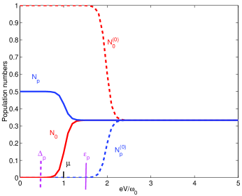
Figure 1: (Color online) Population numbers $N_{0},N_{p}$ for three states: empty state $|0)$ and two degenerate ones $|p_{1}),|p_{2})$, - as a function of the bias voltage. The energies are given in units of confinement energy $\omega_{0}$. The electrochemical potential is chosen at $\mu/\omega_{0}=1.0$ and $T/\omega_{0}=0.033$. The solid (dashed) line displays the behavior of the population number with the renormalized (bare) energy.

IV.1 Shell effects

The response of the QD to applied bias voltage is determined, evidently, by a electronic levels within the conducting window $(\mu_{l},\mu_{r})$. The number of levels in the window depends : i) on the relative position of the bottom of the confinement potential in QD and the equilibrium position of the electrochemical potential ($eV=0$); ii) on the strength of magnetic field. Although the transport properties in the WCI regime are known, we shortly summarize the corresponding effects in order to compare it with the ones in the SCI regime.

The formula for the current for the WCI regime has the same form as Eq.(84), but contains normal width $\Gamma$ instead of effective one $\Gamma P$. Thus, putting formally $P=1$ in Eq.(84), we obtain:

$$J^{WCI}=\frac{4e}{\hbar}\sum_{\gamma}\int d\omega[f_{l}(\omega)-f_{r}(\omega)]\frac{\Gamma_{\gamma}^{l}(\omega)\Gamma_{\gamma}^{r}(\omega)}{[\omega-\varepsilon_{\gamma}]^{2}+[\Gamma_{\gamma}(\omega)]^{2}}.$$ (86)

In the wide-band case, as mentioned above, the width does not depend on energy, $\Gamma_{\gamma}^{l/r}(\omega)\rightarrow\Gamma_{\gamma}^{l/r}$. Then at small dot-lead coupling we find:

$$J_{l}\simeq\frac{4\pi e}{\hbar}\sum_{\gamma}\frac{\Gamma_{\gamma}^{l}\Gamma_{\gamma}^{r}}{\Gamma_{\gamma}}[f_{l}(\varepsilon_{\gamma})-f_{r}(\varepsilon_{\gamma})].$$ (87)

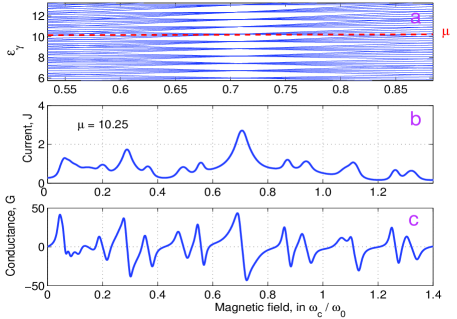
Figure 2: (Color online) Magnetic field dependence ($t=\omega_{c}/\omega_{0}$) of: a) a Fock-Darwin spectrum; the position of the chemical potential $\mu$ is displayed by a dashed line; b)the tunnelling current $J$ through the quantum dot; c)the conductance G. See text for the definition of $J$ and $G$. All energies are given in units of the confinement energy $\omega_{0}$

The shell structure in the spectrum of a QD is evidently observed in the WCI regime (see Fig.2a). We use a fixed value for the confinement energy $\omega_{0}$. The validity of the assumption about the independence of this energy on the number of electrons in the dot, actually, is not obvious at all. We believe, however, that strong enough external confining potential and a small number of electrons (i.e., $\leq 20$) all results would persist, since the magnetic field contributes additionally to the external confining potential.

At given $\mu=(\mu_{L}+\mu_{R})/2$ (that simulates in our case the choice of the gate voltage $V_{gate}$) the number of conducting channels is determined by the number of the Fock-Darwin levels in the conducting window $\mu_{R}<\Delta E<\mu_{L}$ (CW). This number is changing when the magnetic field grows: the levels with higher values of orbital (and spin) momenta $m$ move down faster than those with lower momenta and, therefore, the high-lying levels with large values of $L_{z}=m$ should unavoidably show up in the CW at large enough magnetic field. The levels with the negative orbital momenta $L_{z}=-m^{\prime}$ move up and leave the CW, decreasing, thus, the number of conducting channels. These two processes result in oscillations in the current (see Fig.2b). Thus, each new level entering the CW determined by $\mu-eV/2<\varepsilon_{\gamma}<\mu+eV/2$, produces step in the current with the height $J_{0,\gamma}=4\pi e\Gamma_{\gamma}^{l}\Gamma_{\gamma}^{r}/\left(\hbar\Gamma_{\gamma}\right)$. In a narrow energy interval the widths $\Gamma_{\gamma}$ differ from each other only slightly, $J_{0,\gamma}\approx J_{0}=\pi e\Gamma/\hbar$, then the ”reduced” current $J/J_{0}$ should display integer steps. If some level $\varepsilon_{\gamma}$ is $n_{\gamma}$ times degenerate, the step increases $n_{\gamma}$ times. The effect of degeneracy of the spectrum becomes transparent at the special values of the magnetic field

$$t_{0}\equiv\omega_{c}/\omega_{0}=(k-1)/\sqrt{k},$$ (88)

which are determined by the ratio $\Omega_{+}/\Omega_{-}=k=1,2,3,\ldots$ of the eigen modes of the two-dimensional quantum dot HN (see Fig.3).

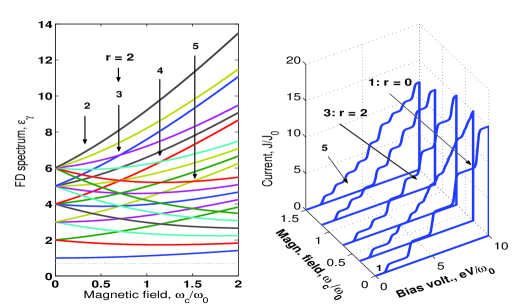
Figure 3: (Color online) Magnetic field ($\omega_{c}/\omega_{0}$) dependence of: the Fock-Darwin spectrum (in units $\omega_{0}$) (left); the tunnelling current $J_{WCI}$ (in units $J_{0}=\bar{\Gamma}/4h$) through the quantum dot (right). Arrows indicate the cuts in the planes that correspond to the fields $\omega_{c}/\omega_{0}=0.0,0.34,0.7$, respectively. The degeneracy at $\omega_{c}/\omega_{0}=0.0,0.7$ is clearly seen in jumps of the current at $T=0$.

At these values the current drastically increases, whereas for the values which are slightly larger than $t_{0}$, the negative differential conductance, $G=dJ/dV$, arises. This is illustrated in fig.2c.

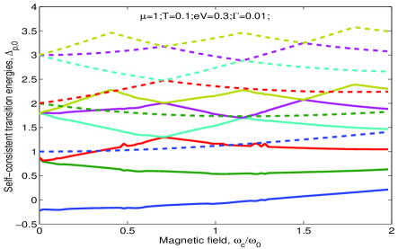
Figure 4: (Color online) The bare (dashed line) and renormalized (solid line) energies as a function of the magnetic field. The parameters of calculations are the same for the WCI and SCI regimes. Five lowest level of the Fock-Darwin spectrum were taken as the bare energies.

Fig.4 displays the renormalized spectrum, obtained from the self-consistent solution of the system of Eqs.(81),(82). As expected from the estimation (83), the renormalization is quite large. Due to a large number of the transitions, contributing into the energy shift (see Eq.(82)), all transition energies are shifted more or less homogeneously. Thus, in spirit, this is, indeed, the MFA: the more transitions contribute into renormalization the closer is the shift of each level to an average value (mean field) (see Fig.4). The most prominent feature caused by these shifts of the transition energies is a decrease of the threshold of the bias voltage to observe the non-zero current. At small $eV$ and chosen fixed $\mu$ (or the gate voltage) the first transition $\Delta_{10}<\mu_{r}$, and the current, Eq.(84), is zero, in spite of $P_{0\gamma}\neq 0$ ($N_{0}=1$) (see Fig.5). At higher voltages the CW contains $n_{W}$ electron states and, according to Eq.(69), $P_{0\gamma}=2/(n_{W}+1)$. As a result, the SCI current is $J_{SCI}=2J_{0}n_{W}/(n_{W}+1)$, where $J_{0}=\pi e\sum_{\gamma}\Gamma_{\gamma}/\left[\hbar n_{W}\right]\equiv\pi e\tilde{\Gamma}/\left(\hbar\right)$. The WCI current, however, is $J_{WCI}=J_{0}n_{W}$. Thus, even for a large bias voltage $eV$, the SCI current is weaker than the WCI one, by factor of $\eta=J_{SCI}/J_{WCI}=2/(n_{W}+1)$ (until the other charge sector is not switched on at $eV\sim U$).

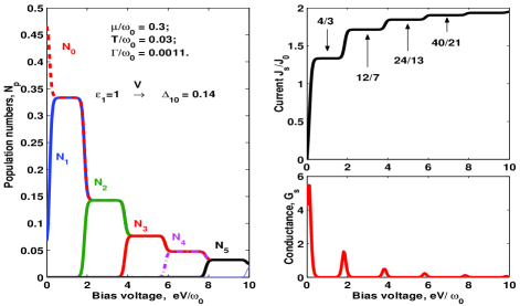
Figure 5: (Color online) Population numbers $N_{p}$ (left panel), the current $J_{S}/J_{0}$ and the conductance $G_{S}=dJ_{S}/d(eV)$ as a function of the bias voltage (right panel) in the SCI regime at zero magnetic field. In each shell $k$ we have $2(k+1)$ degenerate orbitals characterized by the same $N_{p}$ ($p=k+1$). In particular, $N_{0}=<X^{00}>$, $N_{1}=N_{k=0,\gamma_{0}=1}=N_{k=0,\gamma_{0}=2}$ etc, where $\gamma_{k}$ is the orbital index in the shell $k$. Arrows at the bias voltage axis indicate the position of the bare $\varepsilon_{1}$ and the renormalized $\Delta_{10}$ energies from the shell $k=0$. Their exact values and the parameters of the calculations are displayed on the left panel. On the right panel, the rational numbers characterize the height of the $n$-th step in the SCI current, $J_{SCI}/J_{0}=2(n+1)(n+2)/(n^{2}+3n+3)$, for the last filled shell $n$.

Let us compare the manifestation of shell degeneracies defined by the condition, Eq.(88), in nonlinear transport at the WCI and SCI regimes. We consider first $r=1$, i.e., a zero magnetic field (see Fig.3). In this case, each shell $k$ has the degeneracy $g_{k}=k+1$. If in the transport window the last shell $n$ is filled, the total number of states involved into the transport is $n_{W}+1=2\sum_{k=0}^{n}(k+1)+1=n^{2}+3n+3$ (2 is due to the spin degeneracy). Consequently, the height of the $n$-th step in the SCI current is $J_{SCI}/J_{0}=2(n+1)(n+2)/(n^{2}+3n+3)$, which is smaller than the WCI current by factor $\eta=2/(n^{2}+3n+3)$. Since $\Phi_{\gamma}\simeq e^{-\beta\left(\Delta_{\gamma 0}-\mu\right)}\left[1+\alpha\left(eV\right)^{2}\right]$ at small $eV$ (see Eqs.(70)), these effects can not be seen in the linear conductance. Another effect (which is not seen in the master-equation approach) follows from Eq.(81)(see also Fig.1): the coupling pushes the transition energies $\Delta_{\gamma 0}$ down compared to the bare energies $\varepsilon_{\gamma}$, which decreases the bias voltage threshold, as was mentioned above, for the current to be observed. At $r=2$ ($\omega_{c}/\omega_{0}\simeq 0.7$), a new shell structure (see Fig.3) arises as if the confining potential would be a deformed harmonic oscillator without magnetic field. The number of levels are just the number of levels obtained from the 2D oscillator with $\omega_{>}=2\omega_{<}$ ($\omega_{>}$ and $\omega_{<}$ denote the larger and smaller value of the two frequencies). In this case $n_{W}=(n+2)^{2}/2$ if the last filled shell is even, and $n_{W}=(n+1)(n+3)/2$ if it is odd, and these numbers define the heights of steps in both the WCI and SCI regimes.

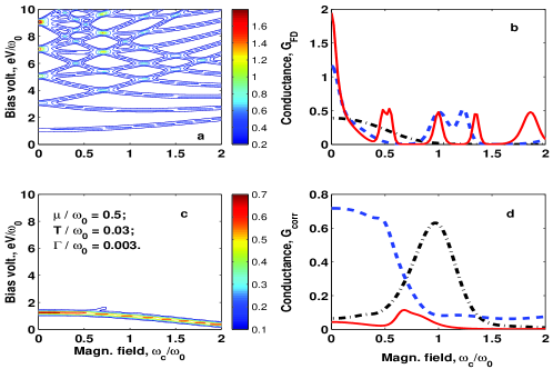
Figure 6: (Color online) The magnetoconductance $G=dJ/(eV)$ at the WCI (left) and the SCI regimes (right). a)The contour plot for the WCI conductance displays the Fock-Darwin spectrum of the parabolic QD in the magnetic field. b)The conductance in the WCI regime, at fixed values of the bias voltage. The results for $eV/\omega_{0}=1,5,9$ are presented by dot-dashed, dashed and solid lines, correspondingly. c)The contour plot for the self-consistent conductance at the SCI regime. d)The self-consistent conductance at the SCI regime, at fixed values of the bias voltage. The dot-dashed, dashed and solid lines present the results for $eV/\omega_{0}=1,1.25,1.45$, correspondingly. The parameters of the calculations are displayed in the panel ”c”.

These features of the spectrum can be traced by means of the conductance measurements (see Fig.6). In particular, the results for the differential conductance $dJ/d(eV)$ at the WCI regime (Fig.6a) resembles very much the experimental conductance discussed in Refs.ota, . The increase of the bias voltage allows to detect the degeneracy of quantum transitions involved in the transport by means of the oscillations in the conductance (see Fig.6b). The large conductance magnitude at zero magnetic field corresponds to the large number of the levels involved in the transport. With the increase of the magnetic field at fixed bias voltage (solid line), the conductance oscillates due to appearance and disappearance of the shells. As was mentioned above, the increase of the magnetic field brings into the CW states with a large magnetic quantum number $m=n_{-}-n_{+}$ and pushes up the ones with $-m$. This gives oscillations in the current (see Fig.2b), which are suppressed, however, together with the current itself in the SCI regime (see Fig.6c).

Let us discuss once more the physical origin of the current and the conductance suppression by the correlations. An increase of the bias-voltage window involves new and new levels (or, more accurately, transition energies) into transportation of electrons through QD. In SCI regime (contrary to the WCI one) all processes are developing under some constraints. First one is that QD cannot contain more than one electron due to a large energy gap between single- and two particle states (our model consideration is performed in the limit $U\rightarrow\infty$). Second constraint comes from the normalization condition: each channel participates in the transport with the spectral weight $P_{\gamma}=N_{0}+N_{\gamma}<1$, whereas the population numbers fulfil the sum rule $=N_{0}+\sum_{\gamma}N_{\gamma}=1$. This automatically leads to the conclusion that the more levels are involved, the less contribution each channel makes into the current and, correspondingly, to the conductance (see Fig.5). Furthermore, since the parabolic QD has a spectrum with the shell structure, the number of involved levels grows very fast. This explains why a strong suppression of the transport by the correlations occurs in very narrow interval of the bias voltage (see Fig.6d). Note that in spite of the strong suppression of the SCI conductance by the intra-dot correlations, it is possible to observe a fine structure produced by the shell structure as well at a certain values of the bias voltage (see Fig.6d).

V Discussion and Summary

In this work we perform an analysis of the non-linear transport through QD, attached to two metallic contacts via insulating/vacuum barriers, in the regime of strong intra-dot Coulomb interaction. The calculation of the current and conductance is based on the formula, derived by Meir and Wingreen MW . It expresses the current in terms of Green functions of fermions in a QD. In the regime of strong Coulomb interaction the fermion variables are not good starting point for a constructing the perturbation theory with respect to the small transparency of the barriers. For this reason we use the approach where an active element (quantum dot) of the device is supposed to be treated as good as possible (ideally, exactly), whereas the coupling to the metallic contacts is treated perturbatively. This leads to description in terms of many-electron operators; particulaly, here we find convenient to use the Hubbard operators. We have re-written the Meir-Wingreen’s formula in terms of Green functions (GFs), defined on Hubbard operators. The Wick’s theorem does not work for such GFs. In our approach this problem is solved by means of the extension of the diagram technique for Hubbard-operator Green functions (developed earlier for a equilibrium in Ref.ig, ) to the non-equilibrium states. In the first step, the exact functional equations for the many-electron GFs are derived and used for the iterations in the spirit of the Schwinger-Kadanoff-Baym approach (see also Ref.ig, ). This gives rise to the diagrammatic expansion. In the second step the analytical continuation of these equations to the real-time axis transforms the system to the non-equilibrium form.

At the limit of infinitely strong intra-dot Coulomb interaction, the lowest approximation with respect to a small transparency of barriers happen to be the mean field theory. In this theory the population numbers of the intra-dot states and the energies of the transition between these states have to be found self-consistently in non-equilibrium (but stationary) states. Thus, the non-equilibrium mean field theory for multiple-level QD has been constructed for non-zero temperature (to the best of our knowledge this is the first attempt in literature). It worth to note that a common practice is to consider the population numbers of many-electron states in the Gibbs’ form (following, e.g., Ref.MW, ). In such an approach the population numbers do depend on the magnetic field, however the dependence on the bias voltage is missing (cf Refs.datta1, ; datta2, ; asano, ).

One of the questions we have addressed in the paper is to what extent the levels (energies of the transitions) of the QD are sensitive to the applied bias voltage $eV$. We have found that this dependence is logarithmically weak (see Eq.83). In contrast, the population numbers manifest much stronger and highly non-trivial dependence on the bias voltage. At zero bias voltage they display the standard Gibbs’ statistics. However, at the voltage higher than a certain critical value (determined by the position of renormalized transition energy) the population numbers start equalizing! This occurs with only those of transitions which have energies within the conducting window $(\mu_{r},\mu_{l})$. This result is obtained analytically in simplified equations and confirmed by the numerical solution of a complete system of non-linear integral equations.

The expression for the current for SCI regime that we have derived (Eq.(84)), demonstrates that the degree of the nonlinearity of the transport is essentially determined by the spectral weights $P_{p}$ of the dot states. Since they are just the sum of the population numbers, $P_{p}=N_{0}+N_{p}$, the non-trivial behavior of the latters (see Eqs.(64),(67),(69)) is reflected in transport properties via a spectral weight of each conducting channel.

Applying further these equations to the problem of the transport through a two-dimensional parabolic quantum dot, we obtain a simple expression which relates the height of the n-th step in the current to the number of states participating in the transport. In the WCI regime, at specific values of the magnetic filed, Eq.(88), we predict a drastic increase of the current through the dot due to the shell effects. Possibly, this effect can be used in applications (i.g., for magnetic-field sensitive switch on-off devices). In the SCI regime the transport is strongly suppressed. The origin of it again is connected with the spectral weights, regulating the contribution of each conducting channel. First, the sum of population numbers is equal to one. Second, the number of levels within the conducting window grows very fast due to existence of the shell structure in the spectrum of parabolic QD. Third, in the limit $U\rightarrow\infty$ the QD cannot contain more than one electron. Therefore, the contribution of each channel unavoidably drops down when expanding by increasing voltage conducting window embraces more and more transition energies. As a result, the current tends to a certain limit, whereas the heights of the peaks in the conductance tend to zero. Thus, we conclude: while in the WCI regime the fine structures in the conductance within one ”diamond” can arise due to re-scattering/co-tunneling processes, in the SCI regime it has the other origin. Namely, the role of single-electron levels is played by the energies of the transition between many-electron states, and the contribution of each transition into transport is regulated by the strength of its coupling to the conduction-electron subsystem and the spectral weights.

Appendix A Relations between Fermi and Hubbard operators

It is convenient to use different notations for Hubbard operators that describe Bose-like transitions (without change of particle numbers) and Fermi-like ones (between the states, differing by one electron). The former and the later ones are denoted as ($Z$) and ($X$), respectively:

$$Z^{00}=\prod_{\gamma_{1}}\left(1-d_{\gamma_{1}}^{\dagger}d_{\gamma_{1}}\right)=\left|0\right\rangle\left\langle 0\right|,\;\;$$ (A.1)

$$Z^{\gamma\gamma}=\prod_{\gamma_{1}\neq\gamma}\left(1-d_{\gamma_{1}}^{\dagger}\gamma_{\gamma_{1}}\right)d_{\gamma}^{\dagger}d_{\gamma}=\left|\gamma\right\rangle\left\langle\gamma\right|,\;\;$$ (A.2)

$$X^{0\gamma}=\prod_{\gamma_{1}\neq\gamma}\left(1-d_{\gamma_{1}}^{\dagger}d_{\gamma_{1}}\right)d_{\gamma}=\left|0\right\rangle\left\langle\gamma\right|,$$ (A.3)

$$Z^{00}\left|0\right\rangle=\left|0\right\rangle,\quad Z^{\gamma\gamma}\left|\gamma\right\rangle=\left|\gamma\right\rangle,$$ (A.4)

where Eq.(A.1) defines the vacuum state and the product is taken over all single-particle states $\gamma_{1}$ of the QD confining potential. In this case the expansion of unity acquires the form:

$$\hat{1}=Z^{00}+\sum_{\gamma}Z^{\gamma\gamma}.$$ (A.5)

The expectation values $N_{0}=\left\langle Z^{00}\right\rangle$ and $N_{\gamma}=\left\langle Z^{\gamma\gamma}\right\rangle$ with respect to state/ensemble of interest are population numbers of corresponding many-electron states. The Hamiltonians of closed QD in these terms become:

$$H_{QD}^{WCI}=\sum_{\gamma}\varepsilon_{\gamma}d_{\gamma}^{\dagger}d_{\gamma},\;\;H_{QD}^{SCI}=\varepsilon_{0}Z^{00}+\sum_{\gamma}\varepsilon_{\gamma}Z^{\gamma\gamma}.$$ (A.6)

The WCI regime corresponds to $U\rightarrow 0$, while the SCI regime takes place at $U\rightarrow\infty$. The energy of empty QD $\varepsilon_{0}$ is determined by the potential depth and can be chosen arbitrarily. While the eigenvalues $\varepsilon_{\gamma}$ are defined by shape of the potential, the transition energies are $\Delta_{\gamma}^{(0)}\equiv$ $\varepsilon_{\gamma}-\varepsilon_{0}$. We recall that the position of the single-electron transitions with respect to the electrochemical potentials is essential for the transport properties of the system.

To write $H_{t}$ in these variables, we have to express the annihilation (creation) operator $d_{\gamma}(d_{\gamma}^{\dagger})$ in terms of Hubbard operators:

$$d_{\gamma}=\hat{1}\cdot d_{\gamma}\cdot\hat{1}=\left\langle 0\right|d_{\gamma}\left|\gamma\right\rangle X^{0\gamma}.$$ (A.7)

Of course, the expansion (A.7) should contain the transitions from one- to two-particle, from two- to three-particle and so on configuration ${\Lambda^{n}}$

$$d_{\gamma}=\sum_{\left\{\Lambda,n\right\}}\left(\Lambda^{(n)},n\left|d_{\gamma}\right|\Lambda^{(n+1)},n+1\right)X^{\Lambda^{(n)}\Lambda^{(n+1)}},$$ (A.8)

that defines the anticommutator relation

$$\hat{1}=\left\{d_{\gamma},d_{\gamma}^{\dagger}\right\}=\sum_{\left\{\Lambda,n\right\}}Z^{\Lambda^{(n)}\Lambda^{(n)}}.$$ (A.9)

However, in the limit $U\rightarrow\infty$ the above equation is reduced to Eq.(A.5). In other words, we consider the transport within the first  conducting ”diamond” only, in coordinates of gate and bias voltages.  The $H_{t}$ remains unchanged in the WCI regime, whereas in the SCI regime it can be written in the form

$$H_{t}^{SCI}=\sum_{k,\sigma\in\lambda,\lambda,\gamma}\left(v_{k\sigma,\gamma}^{\lambda}c_{\lambda k\sigma}^{\dagger}X^{0\gamma}+h.c.\right)$$ (A.10)

where

$$v_{k\sigma;\gamma}^{\lambda}=\tilde{v}_{k\sigma;\gamma}^{\lambda}\langle 0|d_{\gamma}|\gamma\rangle,$$

$$v_{\gamma;k\sigma}^{\lambda}=\tilde{v}_{\gamma;k\sigma}^{\lambda}\langle\gamma|d_{\gamma}^{\dagger}|0\rangle$$ (A.11)

The matrix element $v_{k\sigma;0\gamma}^{\lambda}$ contains information on specific features of attachment between a quantum dot and contacts. Here, $\lambda=l,r$ denotes the left and the right lead, respectively. One may notice that Hubbard operators take into account corresponding kinematic restrictions placed by the strong Coulomb interaction. The prize for this is, however, non-trivial commutation relations:

$$\left\{X^{0\gamma},X^{\gamma^{\prime}0}\right\}=\delta_{\gamma\gamma^{\prime}}Z^{00}+Z^{\gamma^{\prime}\gamma},\;[Z^{00},X^{0\gamma}]=X^{0\gamma},$$

$$[Z^{\gamma^{\prime}\gamma^{\prime\prime}},X^{0\gamma}]=-\delta_{\gamma\gamma^{\prime}}X^{0\gamma^{\prime\prime}}.$$ (A.12)

Thus, our model Hamiltonian takes the form

$$H=\sum_{k\sigma\in\lambda,\lambda}\varepsilon_{\lambda k\sigma}c_{\lambda k\sigma}^{\dagger}c_{\lambda k\sigma}+\varepsilon_{0}Z^{00}+\sum_{\gamma}\varepsilon_{\gamma}Z^{\gamma\gamma}$$

$$+\sum_{k\sigma\in\lambda,\lambda,\gamma}\left(v_{k\sigma,\gamma}^{\lambda}c_{\lambda k\sigma}^{\dagger}X^{0\gamma}+h.c.\right)$$ (A.13)

We assume also that $\{c_{\lambda k\sigma},c_{\lambda^{\prime}k^{\prime}\alpha^{\prime}}^{\dagger}\}=\delta_{k,k^{\prime}}\delta_{\sigma,\sigma^{\prime}}\delta_{\lambda,\lambda^{\prime}},\,\,\{c_{\lambda k\sigma},d_{\gamma}^{\dagger}\}=0$.

As it was discussed in the Introduction, the particular sector of the transitions ($0\Longleftrightarrow 1$) is remarkable due to the fact that the bare energies $\varepsilon_{\gamma}$ and the tunnelling matrix elements coincide in both the WCI and the SCI regimes. This opens a nice opportunity to study the role played by the strong Coulomb interaction in formation of transport properties in a most refined form. Indeed, in the SCI case the electrons in QD can ”see” the conduction electrons in the attached contacts only through the prism of the in-dot kinematic constraints. This results in the renormalization of the transition energies.

Appendix B Current

Here we re-derive the expression for the current obtained by Meir and Wingreen MW in terms of Green functions (GFs) for the Hubbard operators. Thus,

$$J_{l}=\frac{ie}{\hbar}\sum_{k\sigma\in l,\gamma}\left\{\tilde{v}_{k\sigma,0\gamma}^{l}\left\langle c_{lk\sigma}^{\dagger}d_{\gamma}\right\rangle-\tilde{v}_{\gamma 0,k\sigma}^{l}\left\langle d_{\gamma}^{\dagger}c_{lk\sigma}\right\rangle\right\}$$

$$=\frac{ie}{\hbar}\sum_{k\sigma\in l,\gamma}\left\{v_{k\sigma,\gamma}^{l}\left\langle c_{lk\sigma}^{\dagger}X^{0\gamma}\right\rangle-v_{\gamma,k\sigma}^{l}\left\langle X^{\gamma 0}c_{lk\sigma}\right\rangle\right\}$$

$$=\frac{e}{\hbar}\sum_{k\sigma\in l,\gamma}\int d\omega\left\{v_{k\sigma,\gamma}^{l}G_{\gamma,k\sigma}^{<}(\omega)-v_{\gamma,k\sigma}^{l}G_{k\sigma,\gamma}^{<}(\omega)\right\}$$

. (B.1)

where the matrix elements $v_{k\sigma,\gamma}^{l}(v_{\gamma,k\sigma}^{l}$) are defined by Eq.(A.11). Equations for the Green functions $G_{\gamma,k\sigma}$ and $G_{k\sigma,\gamma}$ on the Keldysh contour are

$$G_{\gamma,k\sigma}(\tau,\tau^{\prime}) =\int_{C}d\tau_{1}G_{\gamma,\gamma^{\prime}}(\tau,\tau_{1})v_{\gamma^{\prime},k\sigma}^{l}C_{k\sigma}^{(0)}(\tau_{1},\tau^{\prime})$$ (B.2)

$$G_{k\sigma,\gamma}(\tau,\tau^{\prime}) =\int_{C}d\tau_{1}C_{k\sigma}^{(0)}(\tau,\tau_{1})v_{k\sigma,\gamma^{\prime}}^{l}G_{\gamma^{\prime},\gamma}(\tau,\tau_{1})$$ (B.3)

Here $C_{k\sigma}^{(0)}(\tau_{1},\tau^{\prime})$ is a bare GF of conduction electrons in the left lead. Expressing GFs $G$ via integrals on real-time axes and making a Fourier transformation with respect to a difference of times (the steady state is considered only!), we obtain:

$$G_{\gamma,k\sigma}^{<}(\omega) = G_{\gamma,\gamma^{\prime}}^{<}(\omega)v_{\gamma^{\prime},k\sigma}^{l}C_{k\sigma}^{(0)A}(\omega)+$$

$$+ G_{\gamma,\gamma^{\prime}}^{R}(\omega)v_{\gamma^{\prime},k\sigma}^{l}C_{k\sigma}^{(0)<}(\omega)$$

$$G_{k\sigma,\gamma}^{<}(\omega) = C_{k\sigma}^{(0)<}(\omega)v_{k\sigma,\gamma^{\prime}}^{l}G_{\gamma^{\prime},\gamma}^{A}(\omega)+$$

$$+ C_{k\sigma}^{(0)R}(\omega)v_{k\sigma,\gamma^{\prime}}^{l}G_{\gamma^{\prime},\gamma}^{<}(\omega)$$

Here, the Fourier transformation is defined as:

$$G(t)=\int\frac{d\omega}{2\pi}e^{-i\omega t}G(\omega),G(\omega)=\int dte^{i\omega t}G(t).$$ (B.5)

Inserting Eqs.(LABEL:c5b) into Eq.(B.1), we have:

$$J_{l} =\frac{e}{\hbar}\int d\omega\left[G_{\gamma,\gamma^{\prime}}^{<}(\omega)V_{\gamma^{\prime},\gamma}^{l,A}(\omega)+G_{\gamma,\gamma^{\prime}}^{R}(\omega)V_{\gamma^{\prime}\gamma}^{l,<}(\omega)\right]$$ (B.6)

$$-\frac{e}{\hbar}\int d\omega\left[V_{\gamma\gamma^{\prime}}^{l,<}(\omega)G_{\gamma,\gamma^{\prime}}^{A}(\omega)+V_{\gamma\gamma^{\prime}}^{l,R}(\omega)G_{\gamma,\gamma^{\prime}}^{<}(\omega)\right]$$

Here, we have introduced the effective interaction with conduction electrons in the lead $\lambda=l$:

$$V_{\gamma^{\prime}\gamma}^{\lambda,\eta}(\omega)=\sum_{k\sigma\in\lambda}v_{\gamma^{\prime},k\sigma}^{\lambda}C_{k\sigma}^{(0)\eta}(\omega)v_{k\sigma,\gamma}^{\lambda},$$ (B.7)

where $\eta\equiv\{R,A,>,<\}$. Since in the steady state the current is homogeneous, i.e., $J_{l}=(J_{l}+J_{l})/2=$ $(J_{l}-J_{r})/2$, we can symmetrize Eq.(B.6):

$$J_{l}= \frac{e}{2\hbar}\int d\omega[(V_{\gamma^{\prime},\gamma}^{l,A}(\omega)-V_{\gamma^{\prime},\gamma}^{l,R}(\omega))-$$

$$-(V_{\gamma^{\prime},\gamma}^{r,A}(\omega)-V_{\gamma^{\prime},\gamma}^{r,R}(\omega))]G_{\gamma\gamma^{\prime}}^{<}(\omega)+$$

$$+\frac{e}{2\hbar}\int d\omega(V_{\gamma^{\prime},\gamma}^{l,<}(\omega)-V_{\gamma^{\prime},\gamma}^{r,<}(\omega))\left(G_{\gamma\gamma^{\prime}}^{R}(\omega)-G_{\gamma\gamma^{\prime}}^{A}(\omega)\right)$$

Let us calculate the effective interaction $V_{\gamma^{\prime},\gamma}^{l,\eta}(\omega).$ The conduction-electron ”lesser” and ”greater” GFs for the left lead ($\lambda=l$) or for the right one ($\lambda=r$) are:

$$C_{k\sigma}^{(0)<}(t,t^{\prime}) \equiv i\left\langle c_{\lambda k\sigma}^{\dagger}(t^{\prime})c_{\lambda k\sigma}(t)\right\rangle^{(0)}=ie^{-i\varepsilon_{\lambda k\sigma}(t-t^{\prime})}f_{\lambda}(\varepsilon_{\lambda k\sigma})$$

$$C_{k\sigma}^{(0)>}(t,t^{\prime}) \equiv -i\left\langle c_{\lambda k\sigma}(t)c_{\lambda k\sigma}^{\dagger}(t^{\prime})\right\rangle^{(0)}=$$

$$= -ie^{-i\varepsilon_{\lambda k\sigma}(t-t^{\prime})}f_{\lambda}(-\varepsilon_{\lambda k\sigma})$$

$$C_{k\sigma}^{(0)<}(\omega) = i\int d(t-t^{\prime})e^{i\left(\omega-\varepsilon_{\lambda k\sigma}\right)(t-t^{\prime})}f_{\lambda}(\varepsilon_{\lambda k\sigma})=$$

$$= 2\pi i\delta\left(\omega-\varepsilon_{\lambda k\sigma}\right)f_{\lambda}(\omega)$$

$$C_{k\sigma}^{(0)>}(\omega) = -i\int d(t-t^{\prime})e^{i\left(\omega-\varepsilon_{\lambda k\sigma}\right)(t-t^{\prime})}f_{\lambda}(-\varepsilon_{\lambda k\sigma})=$$

$$= -2\pi i\delta\left(\omega-\varepsilon_{\lambda k\sigma}\right)f_{\lambda}(-\omega)$$

For the retarded and advanced GFs we have

$$C_{k\sigma}^{(0)R}(t,t^{\prime}) \equiv -i\theta(t-t^{\prime})\left\langle\left\{c_{\lambda k\sigma}(t),c_{\lambda k\sigma}^{\dagger}(t^{\prime})\right\}\right\rangle_{\lambda}^{(0)}=$$

$$= -i\theta(t-t^{\prime})e^{-i\varepsilon_{\lambda k\sigma}(t-t^{\prime})}$$

$$C_{k\sigma}^{(0)R}(\omega) = -i\int d(t-t^{\prime})\theta(t-t^{\prime})e^{i\left(\omega-\varepsilon_{\lambda k\sigma}\right)(t-t^{\prime})}=$$

$$= \frac{1}{\omega-\varepsilon_{\lambda k\sigma}+i\delta}$$

$$C_{k\sigma}^{(0)A}(t,t^{\prime}) \equiv i\theta(-t+t^{\prime})\left\langle\left\{c_{\lambda k\sigma}(t),c_{\lambda k\sigma}^{\dagger}(t^{\prime})\right\}\right\rangle_{\lambda}^{(0)}=$$

$$= i\theta(-t+t^{\prime})e^{-i\varepsilon_{\lambda k\sigma}(t-t^{\prime})};$$

$$C_{k\sigma}^{(0)A}(\omega) = i\int d(t-t^{\prime})\theta(-t+t^{\prime})e^{i\left(\omega-\varepsilon_{\lambda k\sigma}\right)(t-t^{\prime})}=$$

$$= \frac{1}{\omega-\varepsilon_{\lambda k\sigma}-i\delta}.$$

As a result, we have

$$\left(V_{\gamma^{\prime}\gamma}^{\lambda,A}(\omega)-V_{\gamma^{\prime}\gamma}^{\lambda,R}(\omega)\right)=$$

$$= \sum_{k\sigma\in\lambda}v_{\gamma^{\prime},k\sigma}^{\lambda}\left[C_{k\sigma}^{(0)A}(\omega)-C_{k\sigma}^{(0)R}(\omega)\right]v_{k\sigma,\gamma}^{\lambda}=$$

$$= 2\pi i\sum_{k\sigma\in\lambda}v_{\gamma^{\prime},k\sigma}^{\lambda}\delta(\omega-\varepsilon_{\lambda k\sigma})v_{k\sigma,\gamma}^{\lambda}=2i\Gamma_{\gamma^{\prime}\gamma}^{\lambda}(\omega)$$

and

$$\left(V_{\gamma^{\prime}\gamma}^{l,<}(\omega)-V_{\gamma^{\prime}\gamma}^{r,<}(\omega)\right)=2i\left(f_{l}(\omega)\Gamma_{\gamma^{\prime}\gamma}^{l}(\omega)-f_{r}(\omega)\Gamma_{\gamma^{\prime}\gamma}^{r}(\omega)\right).$$

With the aid of above equations we can rewrite Eq.(B7) in terms of the width functions:

$$J_{l}=\frac{ie}{\hbar}\sum_{\gamma\gamma^{\prime}}\int d\omega\left\{\left[\Gamma_{\gamma}^{\prime}\gamma^{l}(\omega)-\Gamma_{\gamma^{\prime}\gamma}^{r}(\omega)\right]G_{\gamma\gamma^{\prime}}^{<}(\omega)+\right.$$

$$+\left.\left(f_{l}(\omega)\Gamma_{\gamma^{\prime}\gamma}^{l}(\omega)-f_{r}(\omega)\Gamma_{\gamma^{\prime}\gamma}^{r}(\omega)\right)\left(G_{\gamma\gamma^{\prime}}^{R}(\omega)-G_{\gamma\gamma^{\prime}}^{A}(\omega)\right)\right\}.$$

(B.9)

References

- (1) L. P. Kouwenhoven, C. M. Marcus, P. L. McEuen, S. Tarucha, R. M. Westervelt, and N. S. Wingren, in Mesoscopic Electron Transport, edited by L. P. Kouwenhoven, G. Schön and L. L. Sohn NATO ASI, Ser.E., Vol. 345 (Kluwer, Dordrecht, 1997), pp.105-214.
- (2) S. M. Reimann and M. Manninen, Rev. Mod. Phys. 74, 1283 (2002).
- (3) J. Fransson, O. Eriksson, and I. Sandalov, Phys. Rev. Lett. 88, 226601 (2002).
- (4) L. P. Kouwenhoven, D. G. Austing, and S. Tarucha, Rep. Prog. Phys. 64, 701 (2001).
- (5) D. V. Averin and Yu. V. Nazarov, Phys. Rev. Lett. 65, 2446 (1990).
- (6) S. De Franceschi, S. Sasaki, J. M. Elzerman, W. G. van der Wiel, S. Tarucha, and L. P. Kouwenhoven, Phys. Rev. Lett. 86, 878 (2001).
- (7) D. Goldhaber-Gordon, et.al., Nature, 391, 156 (1998); S. M. Cronenwett, T. H. Oosterkamp, and L. P. Kouwenhoven, Science, 281, 540 (1998).
- (8) M. Pustilnik and L. I. Glazman, J. Phys.: Condens. Matter, 16, R513 (2004); L. I. Glazman and M. Pustilnik, cond-mat/0501007.
- (9) R. Schleser, T. Ihn, E. Ruh, K. Ensslin, M. Tews, D. Pfannkuche, D. C. Driscoll, and A. C. Gossard, Phys. Rev. Lett. 94, 206805 (2005).
- (10) S. Hershfield, J. H. Davies, and J. W. Wilkins, Phys. Rev. Lett. 67, 3720 (1991); B. R. Bulka and S. Lipinski Phys. Rev. B 67, 024404 (2003); R. Lopez and D. Sanchez, Phys. Rev. Lett. 90, 116602 (2003); J. Paaske, A. Rosch, and P. Wolfle Phys. Rev. B 69, 155330 (2004).
- (11) K. Ono, D. G. Austing, Y. Tokura and S. Tarucha, Physica B 314, 450 (2002); T. Ota, K. Ono, M. Stopa, T. Hatano, S. Tarucha, H. Z. Song, Y. Nakata, T. Miyazawa, T. Ohshima, and N. Yokoyama, Phys. Rev. Lett. 93, 066801 (2004).
- (12) S. Tarucha, D. G. Austing, T. Honda, R. J. van der Hage, and L. P. Kouwenhoven, Phys. Rev. Lett. 77, 3613 (1996).
- (13) W. Kohn, Phys. Rev. 123, 1242 (1961).
- (14) Ch. Sikorski and U. Merkt, Phys. Rev. Lett. 62, 2164 (1989).
- (15) Ll. Serra, R. G. Nazmitdinov, and A. Puente, Phys. Rev. B 68, 035341 (2003).
- (16) V. Fock, Z. Phys. 47, 446 (1928); C. G. Darwin, Proc. Cambridge Philos. Soc. 27, 86 (1930).
- (17) M. Dineykhan and R. G. Nazmitdinov, Phys. Rev. B55, 13707 (1997); J. Phys.: Condens. Matter, 11, L83 (1999).
- (18) I. Sandalov, B. Johansson, and O. Eriksson, Int. J. Quantum Chem. 94, 113 (2003) (cond-mat/0011259; see also cond-mat/0011260,0011261).
- (19) A. E. Ruckenstein and S. Schmitt-Rink, Int. Journ. Mod. Phys. B 3, No.12, 83 (1989).
- (20) A. Georges and Y. Meir, Phys. Rev. Lett. 82, 3508 (1999); R. Aguado and D.C. Langreth, Phys. Rev. Lett. 85 , 1946 (2000).
- (21) I. Sandalov and R. G. Nazmitdinov, J. Phys. : Condens. Matter 18, L55 (2006).
- (22) J. Hubbard, Proc. R. Soc. London, Ser. A276, 238 (1963); ibid A277, 237 (1963).
- (23) Y. Meir and N. S. Wingreen, Phys. Rev. Lett. 68, 2512 (1992).
- (24) A. P. Jauho, N. S. Wingreen, and Y. Meir, Phys. Rev. B 50, 5528 (1994).
- (25) P. C. Martin and J. Schwinger, Phys. Rev. 115, 1342 (1959).
- (26) L. P. Kadanoff and G. Baym, Quantum Statistical Mechanics (Addison-Wesley, New York, 1989)
- (27) D.C. Langreth, in Linear and nonlinear electron transport in solids, Vol. 17 of Nato Advanced Study Institute, Series B: Physics, edited by J.T. Devreese and V.E. van Doren (Plenum, New York, 1976), pp.3-32.
- (28) Comparison of perturbation-theory series for the long-range part of Coulomb interaction for fermions and Hubbard operators in terms of functional equations is performed in the unpublished work by I. Sandalov, U. Lundin, O. Eriksson, and B. Johansson, cond-mat/0011260.
- (29) N. S. Simonovic and R. G. Nazmitdinov, Phys. Rev. B 67, 041305(R) (2003)
- (30) W. D. Heiss and R. G. Nazmitdinov, Pis’ma ZETF 68, 870 (1998) [JETP Letters 68, 915 (1998)].
- (31) G. Chen, G. Klimeck, and S. Datta, G. Chen, and W. A Goddard, III, Phys. Rev. B 50, 8035 (1994).
- (32) G. Klimeck, G. Chen, and S. Datta, Phys. Rev. B 50, 2316 (1994).
- (33) Y. Asano, Phys. Rev. B 58, 1414 (1998).