Ginzburg-Landau theory of the liquid-solid interface and nucleation for hard-spheres

Abstract

The Ginzburg-Landau free energy functional for hard-spheres is constructed using the Fundamental Measure Theory approach to Density Functional Theory as a starting point. The functional is used to study the liquid-fcc solid planer interface and the properties of small solid clusters nucleating within a liquid. The surface tension for planer interfaces agrees well with simulation and it is found that the properties of the solid clusters are consistent with classical nucleation theory.

I Introduction

The nature of the liquid-solid interface is of both practical and theoretical significance. From a practical point of view, the interfacial surface tension is, along with the bulk free energies, one of the determining factors controlling nucleation of crystals from solution and plays as well an important role in the closely related phenomena of wetting. However, a complete description of the liquid-solid interface based on fundamental considerations remains a challenging theoretical problem since it requires knowledge of the spatial -dependence of the free energy in highly inhomogeneous systems. Much can be learned from more phenomenological approaches such as phase-field theory and model free energy functionals but a detailed relation of interfacial properties to molecular interaction models requires more fundamental approaches. On the other hand, very detailed approaches such as molecular dynamics and Monte Carlo computer simulation can provide direct microscopic information about interfaces, but theory is required in order to understand the results obtained.

Classical density functional theory (DFT) is based on the fact that the Helmholtz free energy is a unique functional of the average density profileEvans (1979),Hansen and McDonald (1986). It has been used to study liquid-solid interfaces - both coexistence and wetting - almost since its inceptionEvans (1979),Haymet and Oxtoby (1981),Oxtoby and Haymet (1982). The most commonly studied system is that of hard-spheres since many density functional theories work best in this case. Although somewhat artificial, the hard-sphere interaction plays an important role in equilibrium statistical mechanics since more realistic pair interactions can be described based on perturbation theory about the hard-sphere interactionHansen and McDonald (1986) or by developments within DFT inspired by perturbation theoryCurtin and Ashcroft (1986). However, the theories which most accurately described the bulk liquid and solid phases for hard-spheres suffer from a serious technical deficiency in that they allow for configurations in which the spheres overlap - a situation which is excluded on physical grounds and which should manifest itself as a divergence in the free energy for configurations in which the spheres touchOhnesorge et al. (1991). Thus, the liquid-solid interface can only be studied with these theories if either the allowed densities are artificially restricted, as in Curtin (1989); Marr and Gast (1993), or if ad hoc modifications are made to the DFT so as to create the required divergence at overlapOhnesorge et al. (1991, 1994). In recent years, a new class of DFT models, generally known as Fundamental Measure Theory (FMT), have proven successful in a number of applications particularly involving inhomogeneous fluids (e.g., fluids near walls)Rosenfeld (1989),Rosenfeld et al. (1990),Rosenfeld et al. (1997). The FMT approach has the advantage that, by the nature of the models used, the problem of overlapping hard-spheres is automatically solved - overlapping spheres lead to an infinite free energy penalty as one would expect. The goal of this paper is therefore to revisit the problem of the liquid-solid interface for hard-spheres both to further test the generality of the FMT approach and also as a preliminary step towards the study of interfaces for more realistic systems.

Within the DFT-FMT framework, there is still considerable latitude in the level of description of the physical system. A bulk liquid is characterized by a constant average density $\rho\left(\overrightarrow{r}\right)=\overline{\rho}$ while a bulk solid is characterized by a spatially-varying density which must have the symmetry of the underlying crystal lattice. Inhomogeneous systems with either interfaces between different phases or confined geometries necessarily have more complex density profiles involving non-periodic spatial variations. For liquids, this does not not pose too great a challenge but for solids, the superposition of the spatial variations within a unit cell and the larger-scale variations coming from the interface can lead to numerically-intensive calculations  see e.g ref. Ohnesorge et al. (1994). Indeed, a recent application of the DFT-FMT approach to the problem of hard-sphere liquid-solid coexistence has been made and serves to illustrate the difficulty of this approachWarshavsky and Song (2006). In this work, the goal is to use a reduced description whereby a small set of order parameters rather than the fully detailed local densityLutsko (2006). In this sense, the present work follows the spirit of phase field methods. However, the free energy functional is systematically derived from the microscopic description thus eliminating the need for phenomenological assumptions and thus allowing for quantitative predictions.

In the next Section, the elements of DFT and its relation to the Ginzburg-Landau theory are reviewed. The FMT density functionals are also described and the use of these functionals to calculate the elements of the GL free energy functional is presented. In Section III, the properties of the planer liquid-solid interface are determined both by means of parametrized profiles of the density and crystallinity and by numerical solution of the Euler-Lagrange equations. The calculated surface tension is shown to be in reasonable agreement with the results of molecular dynamics and Monte Carlo simulations. The structure and free energy of small solid clusters is also discussed. It is found that the properties of the critical nucleus - its size and the widths of the interfacial region - are well predicted by the results obtained for the planer interface using classical nucleation theory. The last Section summarizes the results and discusses possible refinements of the calculations.

II Theory

II.1 Density functional theory

Density functional theory is based on the fact that the grand potential, the thermodynamic free energy appropriate for a system with constant chemical potential $\mu$, constant temperature $T$ and fixed applied one-body field $\phi\left(\overrightarrow{r}\right)$, can be written as

$$\Omega=F\left[\rho\right]-\int\mu\rho\left(\overrightarrow{r}\right)d\overrightarrow{r}+\int\phi\left(\overrightarrow{r}\right)\rho\left(\overrightarrow{r}\right)d\overrightarrow{r}$$ (1)

where the first term on the right is a unique functional of the local density. Different applied fields will give rise to different density profiles and the fundamental theorem of DFT says that there is a one to one correspondence between applied fields and density profilesEvans (1979),Hansen and McDonald (1986). It follows from this definition that the Helmholtz free energy, $A,$ is

$$A=F\left[\rho\right]+\int\phi\left(\overrightarrow{r}\right)\rho\left(\overrightarrow{r}\right)d\overrightarrow{r}$$ (2)

so that $F\left[\rho\right]$ is the intrinsic contribution to the Helmholtz free energy due to the density profile. For situations in which the applied field is not important - for example, when it only represents the walls of a container, the second term is unimportant in the thermodynamic limit and $F\left[\rho\right]$ is often referred to simply as the Helmholtz free energy.

At fixed field, temperature and chemical potential, the density must minimize the grand potential giving the Euler-Lagrange equation

$$\frac{\delta}{\delta\rho\left(\overrightarrow{r}\right)}F\left[\rho\right]-\mu+\phi\left(\overrightarrow{r}\right)=0.$$ (3)

Given a model for the intrinsic free energy functional, $F\left[\rho\right]$, this gives a closed description of the system which generally takes the form of an integral equation. Most applications of DFT make use of parametrized density profiles so as to reduce the effort needed to determine the density. In general, if the density is given by $\rho\left(\overrightarrow{r}\right)=\rho\left(\overrightarrow{r};\Gamma\right)$, where $\rho\left(\overrightarrow{r};\Gamma\right)$ is some fixed function of the spatial coordinates and the permeates $\Gamma=\left\{\Gamma_{a}\right\}_{a=1}^{n_{\Gamma}}$ , then the Euler-Lagrange equations become

$$\frac{\partial}{\partial\Gamma_{a}}F\left[\rho\right]-\mu\frac{\partial\overline{\rho}}{\partial\Gamma_{a}}+\int\phi\left(\overrightarrow{r}\right)\frac{\delta\rho\left(\overrightarrow{r};\Gamma\right)}{\delta\Gamma_{a}}d\overrightarrow{r}=0.$$ (4)

where the notation indicates that $F\left[\rho\right]=F\left(\Gamma\right)$ is an ordinary function of the parameters. The derivatives are understood to be evaluated holding all parameters constant except $\Gamma_{a}$. Note that if one of the parameters corresponds to the average density, say $\Gamma_{0}=\overline{\rho}$, and if the field is zero (or confined to the boundaries so that it can be neglected in the thermodynamic limit) this gives

$$\frac{\partial}{\partial\overline{\rho}}F\left[\rho\right] = \mu$$ (5)

$$\frac{\partial}{\partial\Gamma_{a}}F\left[\rho\right] = 0,\;\;a>0.$$

The first equation is just the usual relation between the Helmholtz free energy and the chemical potential while the second says that the Helmholtz free energy must be stationary with respect to all of the other parameters.

For a bulk solid corresponding to a Bravais lattice with a single atom per unit cell, the density must have the symmetry of the lattice and so takes the form

$$\rho\left(\overrightarrow{r}\right)=\sum_{n}f\left(\overrightarrow{r}-\overrightarrow{R}_{n}\right)$$ (6)

where $\left\{\overrightarrow{R}_{n}\right\}$ are the lattice vectors. In this case, the average density is

$$\overline{\rho} = \frac{1}{V}\int\rho\left(\overrightarrow{r}\right)d\overrightarrow{r}$$

$$= \overline{\rho}_{latt}\int_{WS}f\left(\overrightarrow{r}\right)d\overrightarrow{r}$$

where the second integral is restricted to the Wigner-Seitz cell and where $\overline{\rho}_{latt}$ is the lattice density, defined as the number of lattice points per unit volume. The integral therefore defines the occupancy, $x_{0}=\overline{\rho}/\overline{\rho}_{latt}$: an occupancy of one means that every lattice site is occupied, a value less than one means that there are some vacancies, a value greater than one means that there are some interstitials. Note that eq.(6) can equivalently be written in terms of Fourier components as

$$\rho\left(\overrightarrow{r}\right)=\sum_{n}\exp\left(i\overrightarrow{K}_{n}\cdot\overrightarrow{r}\right)\widetilde{f}\left(\overrightarrow{K}_{n}\right)$$ (8)

where $\widetilde{f}\left(\overrightarrow{k}\right)$ is the Fourier transform of $f\left(\overrightarrow{r}\right)$ and where $\left\{\overrightarrow{K}_{n}\right\}$ is the set of reciprocal lattice vectors.

A typical parametrization of the density, widely used in practical calculations, is to take $f\left(\overrightarrow{r}\right)$ to be a Gaussian so that

$$f\left(\overrightarrow{r}\right)=x_{0}\left(\frac{\alpha}{\pi}\right)^{3/2}\exp\left(-\alpha r^{2}\right).$$ (9)

There are then three parameters: the average density, $\overline{\rho}$, the width of the Gaussian, $\alpha$, and the lattice density $\overline{\rho}_{latt}$ and the occupancy is just $x_{0}=\overline{\rho}/\rho_{latt}$. In this case, one has $\widetilde{f}\left(\overrightarrow{K}_{n}\right)=\overline{\rho}\exp\left(-K_{n}^{2}/4\alpha\right)$ which, together with the fact that $\overrightarrow{K}_{0}=0$ shows that $\lim_{\alpha\rightarrow 0}\rho\left(\overrightarrow{r};\Gamma\right)=\overline{\rho}$ so that the parametrization of the density encompasses both the Gaussian approximation for the solid and the uniform liquid. For this reason, it is common to take the value of the first non-trivial Fourier component to be a measure of the ”crystallinity”, denoted $m$, giving

$$m=\exp\left(-K_{1}^{2}/4\alpha\right)$$ (10)

so that $m=0$ corresponds to a uniform fluid and $m=1$ to an infinitely localized solid. Real solids have values of $m$ which are close to, but always less than, one.

To study interfacial properties, it is necessary to allow for spatial variation in both the average density and in the crystallinity. Here, we follow Ohensorge, et alOhnesorge et al. (1991) and allow $\overline{\rho}$ and $\alpha$ to vary giving

$$\rho\left(\overrightarrow{r}\right)=\left(\overline{\rho}\left(\overrightarrow{r}\right)/\rho_{latt}\right)\left(\frac{\alpha\left(\overrightarrow{r}\right)}{\pi}\right)^{3/2}\sum_{n}\exp\left(-\alpha\left(\overrightarrow{r}\right)\left(\overrightarrow{r}-\overrightarrow{R}_{n}\right)^{2}\right)$$ (11)

or

$$\rho\left(\overrightarrow{r}\right)=\overline{\rho}\left(\overrightarrow{r}\right)\sum_{n}\exp\left(i\overrightarrow{K}_{n}\cdot\overrightarrow{r}\right)\exp\left(-K_{n}^{2}/4\alpha\left(\overrightarrow{r}\right)\right)$$ (12)

depending on which form of the bulk density is used as a basis for the generalization. These expressions are obviously not equivalent although it will turn out below that within the Ginzburg-Landau framework, the differences are unimportant. An alternative parametrization used by Haymet and OxtobyHaymet and Oxtoby (1981),Oxtoby and Haymet (1982) is

$$\rho\left(\overrightarrow{r}\right)=\delta\rho\left(\overrightarrow{r}\right)+\left(\frac{\alpha\left(\overrightarrow{r}\right)}{\pi}\right)^{3/2}\sum_{n}\exp\left(-\alpha\left(\overrightarrow{r}\right)\left(\overrightarrow{r}-\overrightarrow{R}_{n}\right)^{2}\right)$$ (13)

or

$$\rho\left(\overrightarrow{r}\right)=\delta\rho\left(\overrightarrow{r}\right)+\overline{\rho}_{latt}\sum_{n}\exp\left(i\overrightarrow{K}_{n}\cdot\overrightarrow{r}\right)\exp\left(-K_{n}^{2}/4\alpha\left(\overrightarrow{r}\right)\right)$$ (14)

where it is assumed that $\overline{\rho}_{s}=\overline{\rho}_{latt}$ in the solid. One difficulty with this form is that since $\delta\rho\left(\overrightarrow{r}\right)$ must be allowed to be negative (the liquid is less dense than the solid) there is the unphysical possibility that $\rho\left(\overrightarrow{r}\right)<0$ for some points $\overrightarrow{r}$. The form given in eq.(11) is positive definite thus avoiding this problem.

II.2 Fundamental Measure Theory

The original form of Fundamental Measure Theory as given by RosenfeldRosenfeld (1989),Rosenfeld et al. (1990) is in some sense a development of scaled particle theory. This was further extended by Tarazona, Rosenfeld and others using the important requirement that the known, exact free energy functional be recovered in the one-dimensional limit of the theoryTarazona and Rosenfeld (1997),Rosenfeld et al. (1997),Tarazona (2000). The resulting class of theories has proven successful at describing inhomogeneous hard-sphere fluids including the hard-sphere solid. The theory involves a number of local variables, $n_{\alpha}\left(\overrightarrow{r}_{1}\right)$, which are linear functionals of the local density of the form

$$n_{\alpha}\left(\overrightarrow{r}_{1}\right)=\int d\overrightarrow{r}_{2}\;\rho\left(\overrightarrow{r}_{2}\right)w_{\alpha}\left(\overrightarrow{r}_{12}\right).$$ (15)

The set of weights $w_{\alpha}\left(\overrightarrow{r}_{12}\right)$ include a simple step function $\Theta\left(\frac{\sigma}{2}-r\right)$ which serves to define a local packing fraction

$$\eta\left(\overrightarrow{r}_{1}\right)=\int d\overrightarrow{r}_{2}\;\rho\left(\overrightarrow{r}_{2}\right)\Theta\left(\frac{\sigma}{2}-r_{12}\right)$$ (16)

as evidenced by the fact that in the uniform limit, $\rho\left(\overrightarrow{r}_{2}\right)\rightarrow\overline{\rho}$, one has $\eta\left(\overrightarrow{r}_{1}\right)=\frac{\pi}{6}\overline{\rho}\sigma^{3}$ which is the usual definition of the hard-sphere packing fraction. All of the remaining weighting functions are tensorial dyadics of the form $\widehat{r}\widehat{r}...\widehat{r}\delta\left(r-\frac{\sigma}{2}\right)$ and the resulting variables are written generically as

$$T_{ij...l}\left(\overrightarrow{r}_{1}\right)=\int d\overrightarrow{r}_{2}\;\widehat{r}_{12,i}\widehat{r}_{12,j}...\widehat{r}_{12,l}\delta\left(r_{12}-\frac{\sigma}{2}\right)\rho\left(\overrightarrow{r}_{2}\right).$$ (17)

It will be useful to give simpler names for the first two of these quantities, namely

$$s\left(\overrightarrow{r}_{1}\right) = \int d\overrightarrow{r}_{2}\;\delta\left(r_{12}-\frac{\sigma}{2}\right)\rho\left(\overrightarrow{r}_{2}\right)$$ (18)

$$v_{i}\left(\overrightarrow{r}_{1}\right) = \int d\overrightarrow{r}_{2}\;\widehat{r}_{12,i}\delta\left(r_{12}-\frac{\sigma}{2}\right)\rho\left(\overrightarrow{r}_{2}\right)$$

where the names stand for ”scalar” and ”vector” respectively.

The Helmholtz free energy functional is written as

$$F\left[\rho\right]=F_{id}\left[\rho\right]+F_{ex}\left[\rho\right]$$ (19)

where the ideal part of the free energy is

$$\beta F_{id}\left[\rho\right]=\int d\overrightarrow{r}\;\left(\rho\left(\overrightarrow{r}\right)\ln\rho\left(\overrightarrow{r}\right)-\rho\left(\overrightarrow{r}\right)\right)$$ (20)

with $\beta=1/(k_{B}T)$, and the excess contribution is written in the FMT as the integral of a function of the local variables

$$\beta F_{ex}\left[\rho\right]=\int d\overrightarrow{r}\;\beta\phi\left(\left\{n_{\alpha}\left(\overrightarrow{r}\right)\right\}\right)$$ (21)

which is usually expressed as

$$\phi=\phi_{1}+\phi_{2}+\phi_{3}$$ (22)

with

$$\beta\phi_{1} = -\frac{1}{\pi\sigma^{2}}s\left(\overrightarrow{r}\right)\ln\left(1-\eta\left(\overrightarrow{r}\right)\right)$$ (23)

$$\beta\phi_{2} = \frac{1}{2\pi\sigma}\frac{s^{2}\left(\overrightarrow{r}\right)-v^{2}\left(\overrightarrow{r}\right)}{\left(1-\eta\left(\overrightarrow{r}\right)\right)}$$

The form of $\phi_{3}$ depends on the particular version of FMT. Here, three common theories will be considered. The first theory was proposed by Rosenfeld et alRosenfeld et al. (1997) and is perhaps the simplest form of FMT capable of giving a good description of the hard-sphere solid

$$\beta\phi_{3}^{RLST}=\frac{\frac{1}{3}s^{3}\left(\overrightarrow{r}\right)}{8\pi\left(1-\eta\left(\overrightarrow{r}\right)\right)^{2}}\left(1-\frac{v^{2}\left(\overrightarrow{r}\right)}{s^{2}\left(\overrightarrow{r}\right)}\right)^{3}.$$ (24)

The second is the theory of TarazonaTarazona (2000) which makes use of a tensor variable

$$\beta\phi_{3}^{T}=\frac{3}{16\pi}\frac{1}{\left(1-\eta\left(\overrightarrow{r}\right)\right)^{2}}\left(\overrightarrow{v}\left(\overrightarrow{r}\right)\cdot\overleftrightarrow{T}\left(\overrightarrow{r}\right)\cdot\overrightarrow{v}\left(\overrightarrow{r}\right)-s\left(\overrightarrow{r}\right)v^{2}\left(\overrightarrow{r}\right)-Tr\left(\overleftrightarrow{T}^{3}\left(\overrightarrow{r}\right)\right)+s\left(\overrightarrow{r}\right)Tr\left(\overleftrightarrow{T}^{2}\left(\overrightarrow{r}\right)\right)\right).$$ (25)

Both of these theories have the property that they reduce to the Percus-Yevik approximation for the liquid. The third theory builds in the more accurate Carnahan-Starling equation of state via a heuristic modification of the Tarazona theoryTarazona (2002),Roth et al. (2002). It is commonly known as the ”White Bear” functional and is given by

$$\beta\phi_{3}^{WB}=\frac{2}{3}\frac{\eta\left(\overrightarrow{r}\right)+\left(1-\eta\left(\overrightarrow{r}\right)\right)^{2}\ln\left(1-\eta\left(\overrightarrow{r}\right)\right)}{\eta^{2}\left(\overrightarrow{r}\right)}\phi_{3}^{T}.$$ (26)

All three of these theories have deficiencies. The RLST theory incorporates the Percus-Yevik approximation for the liquid which is not very accurate at the density of liquid-solid coexistence. To the extent that the RLST theory gives a good description of liquid-solid coexistence (see below), it is because it gets the liquid and solid “equally wrong”. The Tarazona theory also reduces to the Percus-Yevik approximation for the homogeneous fluid but it gives a better description of the properties of the homogeneous solid leading to a poor description of coexistenceTarazona (2002). For this reason, this theory has not been used in the present investigation. The White Bear (WB) functional gives an improved description of the dense fluid by incorporating the Carnahan-Starling equation of state in an ad hoc fashion. As a result, the implied pair distribution function for the fluid, obtained via the Ornstein-Zernike equation, will not vanish in the core region as it should. Nevertheless, the free energy does diverge for overlapping hard-spheres as in the other forms of FMT. The conclusion is that the RLST is probably the best theory in terms of the formal properties of the free energy while the WB may be expected to be the better in terms of quantitative results.

II.3 Ginzburg-Landau theory

If it can be assumed that the order parameters vary slowly over atomic length scales, a simplified free energy functional can be rigorously derived from the exact free energy functional by means of a gradient expansion in the order parameters. When carried out to second order, the result takes the form of a phenomenological Ginzburg-Landau free energy functionalEvans (1979),Haymet and Oxtoby (1981),Oxtoby and Haymet (1982),Löwen et al. (1989),Löwen et al. (1990),Lutsko (2006),

$$\beta\Omega_{GL}\left[\Gamma\right]=\int d\overrightarrow{R}\;\left[\frac{1}{V}\beta F\left(\Gamma\left(\overrightarrow{R}\right)\right)-\beta\mu\overline{\rho}\left(\Gamma\left(\overrightarrow{R}\right)\right)+\frac{1}{2}K_{ij}^{ab}\left(\Gamma\left(\overrightarrow{R}\right)\right)\frac{\partial\Gamma_{a}\left(\overrightarrow{R}\right)}{\partial R_{i}}\frac{\partial\Gamma_{b}\left(\overrightarrow{R}\right)}{\partial R_{j}}\right]$$ (27)

where the mean field term $\beta F\left(\Gamma\right)$ is the free energy of a bulk system evaluated with order parameters $\Gamma$ and

$$\overline{\rho}\left(\Gamma\right)=\int\rho\left(\overrightarrow{r}_{1};\Gamma\right)d\overrightarrow{r}_{1}.$$

The coefficient of the gradient term is

$$K_{ij}^{ab}\left(\Gamma\right)=\frac{1}{2V}\int d\overrightarrow{r}_{1}d\overrightarrow{r}_{2}\;r_{12i}r_{12j}c_{2}\left(\overrightarrow{r}_{1},\overrightarrow{r}_{2};\Gamma\right)\frac{\partial\rho\left(\overrightarrow{r}_{1};\Gamma\right)}{\partial\Gamma_{a}}\frac{\partial\rho\left(\overrightarrow{r}_{2};\Gamma\right)}{\partial\Gamma_{b}}.$$ (28)

where the direct correlation function is also evaluated for a bulk system with constant order parameters and is determined from the free energy via the standard relation

$$c_{2}\left(\overrightarrow{r}_{1},\overrightarrow{r}_{2};\Gamma\right)=-\frac{\delta^{2}\beta F_{ex}\left[\rho\right]}{\delta\rho\left(\overrightarrow{r}_{1};\Gamma\right)\delta\rho\left(\overrightarrow{r}_{2};\Gamma\right)}.$$ (29)

As discussed in ref.Lutsko (2006), this expression is derived under the assumption that the lattice structure is held fixed. This precludes the use of any characteristics of the lattice, such as the lattice constants or the primitive lattice vectors, as order parameters. Nevertheless, it is possible to explore the liquid-solid interface since, as discussed above, this can be done for a fixed lattice structure.

When the underlying lattice has cubic symmetry, as will be the case here, and in a coordinate system aligned with the principle axes of the lattice structure, the symmetry under 90 degree rotations around the axes implies that the coefficient of the gradient term can be written as

$$K_{ij}^{ab}=g_{ab}\delta_{ij}+h_{ab}\left(\delta_{ix}\delta_{jy}+\delta_{iy}\delta_{jx}+\delta_{ix}\delta_{jz}+\delta_{iz}\delta_{jx}+\delta_{iy}\delta_{jz}+\delta_{iz}\delta_{jy}\right)$$ (30)

where

$$g_{ab}\left(\Gamma\right) = \frac{1}{6V}\int d\overrightarrow{r}_{1}d\overrightarrow{r}_{2}\;r_{12}^{2}c_{2}\left(\overrightarrow{r}_{1},\overrightarrow{r}_{2};\Gamma\right)\frac{\partial\rho\left(\overrightarrow{r}_{1};\Gamma\right)}{\partial\Gamma_{a}}\frac{\partial\rho\left(\overrightarrow{r}_{2};\Gamma\right)}{\partial\Gamma_{b}}$$ (31)

$$h_{ab}\left(\Gamma\right) = \frac{1}{4V}\int d\overrightarrow{r}_{1}d\overrightarrow{r}_{2}\;r_{12x}r_{12y}c_{2}\left(\overrightarrow{r}_{1},\overrightarrow{r}_{2};\Gamma\right)\frac{\partial\rho\left(\overrightarrow{r}_{1};\Gamma\right)}{\partial\Gamma_{a}}\frac{\partial\rho\left(\overrightarrow{r}_{2};\Gamma\right)}{\partial\Gamma_{b}}.$$

To apply this formalism to the FMT, note that the direct correlation function takes the form

$$c_{2}\left(\overrightarrow{r}_{1},\overrightarrow{r}_{2};\Gamma\right)=-\sum_{\alpha,\beta}\int d\overrightarrow{r}\;\frac{\partial^{2}\phi\left(\left\{n_{\alpha}\left(\overrightarrow{r}\right)\right\}\right)}{\partial n_{\alpha}\partial n_{\beta}}w_{\alpha}\left(\overrightarrow{r}-\overrightarrow{r}_{1}\right)w_{\beta}\left(\overrightarrow{r}-\overrightarrow{r}_{2}\right)$$ (32)

At first, it appears that the evaluation of the matrix $K_{ij}^{ab}$ will involve triple volume integrals making it extremely expensive to calculate. However, it is in fact possible to arrange the calculate so that it takes no more effort to calculate $K_{ij}^{ab}$ than is required to calculate the free energy. To do this, note that the calculation requires evaluation of the integral

$$\int d\overrightarrow{r}_{1}d\overrightarrow{r}_{2}\;r_{12i}r_{12j}w_{\alpha}\left(\overrightarrow{r}-\overrightarrow{r}_{1}\right)w_{\beta}\left(\overrightarrow{r}-\overrightarrow{r}_{2}\right)\frac{\partial\rho\left(\overrightarrow{r}_{1};\Gamma\right)}{\partial\Gamma_{a}}\frac{\partial\rho\left(\overrightarrow{r}_{2};\Gamma\right)}{\partial\Gamma_{b}}$$ (33)

which can be simplified by introducing some additional functionals of the density. Specifically, let

$$n_{\alpha}^{i}\left(\overrightarrow{r}\right) = \int d\overrightarrow{r}_{1}\;r_{1i}w_{\alpha}\left(\overrightarrow{r}-\overrightarrow{r}_{1}\right)\rho\left(\overrightarrow{r}_{1};\Gamma\right)$$ (34)

$$n_{\alpha}^{ij}\left(\overrightarrow{r}\right) = \int d\overrightarrow{r}_{1}\;r_{1i}r_{1j}w_{\alpha}\left(\overrightarrow{r}-\overrightarrow{r}_{1}\right)\rho\left(\overrightarrow{r}_{1};\Gamma\right)$$

so that the full expression for $K_{ij}^{ab}$ becomes

$$K_{ij}^{ab}\left(\Gamma\right)=-\frac{1}{2V}\sum_{\alpha,\beta}\int d\overrightarrow{r}\;\frac{\partial^{2}\phi\left(\left\{n_{\alpha}\left(\overrightarrow{r}\right)\right\}\right)}{\partial n_{\alpha}\partial n_{\beta}}\left(\begin{array}[]{c}\frac{\partial n_{\alpha}^{ij}\left(\overrightarrow{r}\right)}{\partial\Gamma_{a}}\frac{\partial n_{\beta}\left(\overrightarrow{r}\right)}{\partial\Gamma_{b}}+\frac{\partial n_{\alpha}\left(\overrightarrow{r}\right)}{\partial\Gamma_{a}}\frac{\partial n_{\beta}^{ij}\left(\overrightarrow{r}\right)}{\partial\Gamma_{b}}\\ -\frac{\partial n_{\alpha}^{i}\left(\overrightarrow{r}\right)}{\partial\Gamma_{a}}\frac{\partial n_{\beta}^{j}\left(\overrightarrow{r}\right)}{\partial\Gamma_{b}}-\frac{\partial n_{\alpha}^{j}\left(\overrightarrow{r}\right)}{\partial\Gamma_{a}}\frac{\partial n_{\beta}^{i}\left(\overrightarrow{r}\right)}{\partial\Gamma_{b}}\end{array}\right).$$ (35)

This is of the same structural form as the expression for the excess free energy, namely a spatial integral involving functions of the local density functionals, and can therefore be evaluated as easily. Furthermore, note that for the tensorial densities, one has

$$T_{ij...l}^{m}\left(\overrightarrow{r}\right) = \left(\frac{\sigma}{2}\right)T_{ij...lm}\left(\overrightarrow{r}\right)$$ (36)

$$T_{ij...l}^{mn}\left(\overrightarrow{r}\right) = \left(\frac{\sigma}{2}\right)^{2}T_{ij...lmn}\left(\overrightarrow{r}\right)$$

The only other quantities needed to evaluate the GL free energy functional are $\eta^{i}\left(\overrightarrow{r}\right)$ and $\eta^{ij}\left(\overrightarrow{r}\right)$. Thus, for the RLST theory, the tensorial quantities must be evaluated up to third order while the White Bear theory requires the fourth order tensor as well. Explicit expressions for all of these quantities are given in Appendix A. An interesting analytic result, proven in Appendix B is that in the RLST theory $h_{ab}\left(\Gamma\right)=0$. Using the WB theory, it is possible that $h_{ab}\left(\Gamma\right)\neq 0$ but the present calculations for the case of an FCC lattice are that the calculated values are so small that neglect of $h_{ab}\left(\Gamma\right)$ makes no difference to the results reported below. Thus, for all practical purposes, the GL free energy functional is not affected by the anisotropy of the underlying lattice for hard spheres.

II.4 Numerical methods

Many quantities, such as the density, can be evaluated either in real space or in Fourier space. Generally, the former is more efficient in the (large $\alpha$) crystalline state and the latter in the (small $\alpha$) liquid state. For the present study, both methods have been used in the calculation of the density and of all of the reqiured density functionals (see Appendix A for details). The implementation was checked by comparing both methods for values of $\alpha a^{2}\sim 20$, where $a=\left(4/\overline{\rho}_{latt}\right)^{1/3}$ is the FCC lattice paramter. In all subsequent calculations, the Fourier-space method was used for $\alpha a^{2}<20$ and the real space method otherwise.

The spatial integrals were evaluated in a limited volume. Specifically, in a homogeneous system, one has that

$$\frac{1}{V}\int d\overrightarrow{r}\;\beta\phi\left(\left\{n_{\alpha}\left(\overrightarrow{r}\right)\right\}\right)=\int_{cell}d\overrightarrow{r}\;\beta\phi\left(\left\{n_{\alpha}\left(\overrightarrow{r}\right)\right\}\right)/\int_{cell}d\overrightarrow{r}\;$$

where the integrals on the right are restricted to the conventional unit cell. For the FCC lattice, elementary symmetry considerations show that the integral on the right can be restricted to the volume $x,y,z>0$ and $x\geq y$ with a symmetry factor of $16$. Further restrictions are possibleGroh and Mulder (2000) but were not used. The integrals were then evaluated using an evenly spaced grid of $20$ points in each direction ( e.g $x=n\delta x/21$ for $0\leq n\leq 20$) . Increasing the number of points had no significant effect on the calculations.

These calculations are still time consuming, especially at intermediate values of $\alpha$, so both $\beta F\left(\Gamma\right)$ and $K_{ij}^{ab}\left(\Gamma\right)$ were evaluated over a grid of points in parameter space and bi-cubic spline interpolationPress et al. (1993) used in the subsequent calculations. Note that since all of the elementary density functionals are linear in the average density, it is possible to perform the calculations for fixed $\alpha$ but many values of the average density at once, i.e. in parallel, thus saving time. One problem is that these quantities, especially $K_{ij}^{ab}\left(\Gamma\right)$, are divergent at high average densities since, for sufficiently high average density, the local packing fraction $\eta\left(\overrightarrow{r}\right)$can exceed one which is just the signal of overlapping hard-spheres. For a homogeneous crystal, the value of the local density for which this divergence occurs is given by $\overline{\rho}_{latt}/\overline{\eta}\left(0\right)$, where $\overline{\eta(r)}$ is defined in Appendix A and given explicitly in eq.(69). This maximum density is always greater than $\overline{\rho}_{latt}$ and approaches $\overline{\rho}_{latt}$ in the limit $\alpha\rightarrow\infty$. Since most of the variation as a function of $\overline{\rho}$ occurs near the maximum value, the procedure used was to discretize the density as

$$\overline{\rho}_{k}=\left\{\begin{array}[]{c}k\rho_{\max}/k_{\max},\;\;k<k_{\max}/2\\ \rho_{\max}-\frac{1}{2}\rho_{\max}\exp\left(\left(\frac{2k-k_{\max}}{k_{\max}}\right)\right),\;\;k>=k_{\max}/2\end{array}\right.$$

with $\rho_{\max}$ chosen to be slightly below $\overline{\rho}_{latt}/\overline{\eta}\left(0\right)$. In the calculations reported below, 200 points were used for the density and the crystallinity was sampled on an evenly spaced grid of 80 points in the range $0\leq m\leq 0.95$.

Some analytic checks on the numerical calculations are possible. Note that the density can be written as

$$\rho\left(\overrightarrow{r}\right) = \overline{\rho}\sum_{j}\exp\left(-k_{j}^{2}/4\alpha\right)\exp\left(i\overrightarrow{K}_{j}\cdot\overrightarrow{r}\right)$$

$$= \overline{\rho}\sum_{j}m^{\left(k_{j}^{2}/k_{1}^{2}\right)}\exp\left(i\overrightarrow{K}_{j}\cdot\overrightarrow{r}\right)$$

$$= \overline{\rho}+\overline{\rho}m\sum_{j\in S_{1}}\exp\left(i\overrightarrow{K}_{j}\cdot\overrightarrow{r}\right)+\overline{\rho}m^{\left(k_{2}^{2}/k_{1}^{2}\right)}\sum_{j\in S_{s}}\exp\left(i\overrightarrow{K}_{j}\cdot\overrightarrow{r}\right)+....$$

where $S_{n}$ is the set of n-th shell reciprocal lattice vectors. It immediately follows that, in the liquid limit, one has

$$\lim_{m\rightarrow 0}\frac{\partial\rho\left(\overrightarrow{r};\Gamma\right)}{\partial\overline{\rho}} = 1$$ (38)

$$\lim_{m\rightarrow 0}\frac{\partial\rho\left(\overrightarrow{r};\Gamma\right)}{\partial m} = \overline{\rho}\sum_{j\in S_{1}}\exp\left(i\overrightarrow{K}_{j}\cdot\overrightarrow{r}\right).$$

giving

$$\lim_{m\rightarrow 0}g_{\rho\rho}\left(\Gamma\right) = \frac{2}{3}\pi\int_{0}^{\infty}r^{4}c_{2}^{l}\left(r;\overline{\rho}\right)dr$$ (39)

$$\lim_{m\rightarrow 0}g_{\rho m}\left(\Gamma\right) = 0$$

$$\lim_{m\rightarrow 0}g_{mm}\left(\Gamma\right) = \frac{2}{3}\pi\overline{\rho}^{2}N_{1}\int_{0}^{\infty}r^{4}c_{2}^{l}\left(r;\overline{\rho}\right)\frac{\sin k_{1}r}{k_{1}r}dr.$$

where $c_{2}^{l}\left(r_{12};\overline{\rho}\right)$ is the direct correlation function of the liquid, $k_{1}$ is the magnitude of the radius of the first shell of the reciprocal lattice and $N_{1}$ is the number of elements in the first shell. For an FCC lattice in real space, the reciprocal lattice is BCC giving $N_{1}=8$ and $K_{1}=\left(\frac{4\pi}{a}\right)\sqrt{3/4}$. With the RLST theory, the dcf of the liquid is just the Percus-Yevik dcf,

$$c_{2}^{PY}\left(r_{12};\overline{\rho}\right)=\left(a_{0}^{py}+a_{1}^{py}\frac{r}{\sigma}+a_{2}^{py}\left(\frac{r}{\sigma}\right)^{3}\right)\Theta\left(r-\sigma\right),$$ (40)

with coefficients

$$a_{0}^{py} = -\frac{\left(1+2\eta\right)^{2}}{\left(1-\eta\right)^{4}}$$ (41)

$$a_{1}^{py} = 6\eta\frac{\left(1+2\eta\right)^{2}}{\left(1-\eta\right)^{4}}$$

$$a_{2}^{py} = \frac{1}{2}\eta a_{0}$$

whereas the White Bear functional gives the same functional form but with coefficientsRoth et al. (2002)

$$a_{0}^{wb} = -\frac{1+\eta\left(4+\eta\left(3-2\eta\right)\right)}{\left(1-\eta\right)^{4}}$$ (42)

$$a_{1}^{wb} = \left(\frac{2-\eta+14\eta^{2}-6\eta^{3}}{\left(1-\eta\right)^{4}}+\frac{2\ln\left(1-\eta\right)}{\eta}\right)$$

$$a_{2}^{wb} = -\left(\frac{3+5\eta\left(\eta-2\right)\left(1-\eta\right)}{\left(1-\eta\right)^{4}}+\frac{2\ln\left(1-\eta\right)}{\eta}\right).$$ (43)

Equations (39)-(43) give a useful check on the full numerical calculation.

Except for the cases explicitly discussed above, all numerical integrals, minimizations and the solution of ordinary differential equations were performed using routines from the Gnu Scientific LibraryGSL . One-dimensionsal minimizations were perfomed using either Brent’s method or bisection while numerical integrals were performed using adaptive integration (the GSL “QAGS” routineGSL ) with relative and absolute accuracies set to $10^{-4}$. Multidimensional minimizations were performed using the Simplex algorithm of Nelder and Mead, see e.g. ref. Press et al. (1993), as implemented in GSL, which was terminated whent the simplex size was smaller than $10^{-4}$.

III Results

III.1 Bulk coexistence

As a baseline for the interfacial calculations, it is necessary to know the predictions of the various theories for the liquid-solid transition. Using the Gaussian parametrization for the density, eqs.(6)-(9), the expressions given above for the free energy are evaluated and, in accord with eq.(5), minimized with respect to $\alpha$ and the lattice density $\rho_{latt}$while the average density must be adjusted so as to satisfy the relation between the free energy and the chemical potential given in eq.(5). One minimum is always found at $\alpha=0$ corresponding to the uniform liquid having density $\overline{\rho}_{l}\left(\mu\right)$. Another occurs at $\alpha_{s}>0$ corresponding to a bulk solid having some average density $\overline{\rho}_{s}\left(\mu\right)$. The true equilibrium is whichever of these solutions that minimizes the grand potential: bulk coexistence occurs when they give identical values

$$\frac{1}{V}\beta F\left(\overline{\rho}_{l}\left(\mu\right),0\right)-\beta\mu\overline{\rho}_{l}\left(\mu\right)=\frac{1}{V}\beta F\left(\overline{\rho}_{s}\left(\mu\right),\alpha_{s}\right)-\beta\mu\overline{\rho}_{s}\left(\mu\right)$$ (44)

or, using eq.(5) and the definition of the pressure, $\beta P=\frac{\partial}{\partial V}\beta F$

$$\beta P\left(\overline{\rho}_{l}\left(\mu\right),0\right)=\beta P\left(\overline{\rho}_{s}\left(\mu\right),\alpha_{s}\right)$$ (45)

which is the usual condition of coexistence. The results for the RLST and WB theories are shown in Table 1 as well as the values from previous calculations and the values from simulation. These numbers are on the whole constant with those in the literature, particularly when it is noted that the calculations reported in the literature were performed with the occupancy fixed to be one. The one exception to this general agreement is the RLST theory where the present results differ noticeably from those reported by Rosenfeld et al.Rosenfeld et al. (1997). However, as an independent check, the evaluations of Warshavsky and SongWarshavsky and Song (2006) are also shown and are seen to be consistent with the present calculations thus supporting the accuracy of the present evaluations.

Table 1: The solid density $\overline{\rho}_{sol}\sigma^{3}$, liquid density $\overline{\rho}_{liq}\sigma^{3}$, reduced pressure $\beta P\sigma^{3}$ and chemical potential $\mu$ at bulk coexistence as determined from (a) the present work, (b)Rosenfeld et al Rosenfeld et al. (1997), (c) Warshavsky and Song Warshavsky and Song (2006), (d) Roth et al.Roth et al. (2002) and (e) from the simulations of Hoover et alHoover and Ree (1968).

Theory	$\overline{\rho}_{sol}\sigma^{3}$	$\overline{\rho}_{liq}\sigma^{3}$	$\beta P\sigma^{3}$	$\mu$
RLST(a)	$1.017$	$0.935$	$12.18$	$16.88$
RLST(b)	$1.031$	$0.938$	$12.3$	17.05
RLST(c)	$1.020$	$0.937$	$12.26$	16.99
WB(a)	$1.022$	$0.932$	$11.20$	15.67
WB(c)	$1.023$	$0.934$	$11.29$
WB(d)	$1.023$	$0.934$
MD(e)	$1.040$	$0.940$	$11.70$

III.2 The planer interface

The simplest application of the theory is to the planer liquid-solid interface. The order parameters are assumed to vary in only one direction, which is writen as $u=\overrightarrow{r}\cdot\widehat{n}$ where $\widehat{n}$ is the normal to the interface, from a bulk solid in the limit $u\rightarrow-\infty$ to a bulk liquid at $u\rightarrow\infty$. For these calculations, the GL free energy functional takes the form

$$\beta\Omega_{GL}^{(Planer)}\left[\Gamma\right]=A\int_{-\infty}^{\infty}du\;\left[\frac{1}{V}\beta F\left(\Gamma\left(u\right)\right)-\beta\mu\overline{\rho}+\frac{1}{2}\left(g_{ab}\left(\Gamma\left(u\right)\right)+2h_{ab}\left(\Gamma\left(u\right)\right)\left(\widehat{n}_{x}\widehat{n}_{y}+\widehat{n}_{x}\widehat{n}_{z}+\widehat{n}_{y}\widehat{n}_{z}\right)\right)\Gamma_{a}^{\prime}\left(u\right)\Gamma_{b}^{\prime}\left(u\right)\right]$$ (46)

where $A$ is the area in the x-y plane. The calculations were performed for a fixed lattice structure at the lattice density appropriate for bulk phase coexistence as determined above.

It is important to realize that the liquid-solid interface is only stable for a unique value of chemical potential. This is because the interface is expected to be a localized structure that decays towards the bulk phases exponentially as one moves away from the interfaceShiryayev and Gunton (2004). However, since the bulk free energy function, $\beta F\left(\Gamma\right)$, and the matrices $g_{ab}\left(\Gamma\right)$ and $h_{ab}\left(\Gamma\right)$ are being approximated via interpolation of tabulated values, it is unlikely that the coexistence properties will be exactly the same as found above. Therefore, a necessary step is to determine coexistence at this fixed lattice structure using the interpolated $\beta F\left(\Gamma\right)$. The procedure used was as follows. Given an initial guess of $\overline{\rho}_{sol}$, the value of $\alpha_{sol}$ was determined by finding the minimum of $\beta F\left(\overline{\rho}_{sol},\alpha\right)$. From this, the chemical potential is determined from the thermodynamic relation, eq.(5) where it is important that the derivative is taken at constant $\alpha$ and $\overline{\rho}_{latt}$. Then, the liquid density is determined from the requirement that $\beta F\left(\overline{\rho}_{liq},0\right)$ give the same chemical potential. Finally, the bulk pressures, $\frac{1}{V}\beta F\left(\Gamma\right)-\beta\mu\overline{\rho}$, are compared for the liquid and solid and the difference used to adjust the value of $\overline{\rho}_{sol}$. The process is iterated until a value of $\overline{\rho}_{sol}$ is found that results in equal pressures between the bulk phases. The results of the bulk calculations are given in Table 2 where the “exact” calculations and those based on the interpolaton scheme are seen to be in good agreement.

One interesting quantity displayed in this table is the difference between the lattice density and the average density. The values given for the RLST theory are in reasonable agreement with the asymptotic values obtained analytically by GrohGroh (2000). However, the WB theory gives a small but negative difference in densities which would mean that instead of vacancies, the theory predicts interstitials. This surprising and unphysical result could be an artifact of the WB theory (which, as discussed above, is an ad hoc extension of Tarazona’s theory) or it could be a numerical artifact indicating that the true vacancy concentration is too small to be reliably calculated with the numerical methods used. Decreasing the tolerances of the numerical evaluations in these calculations did not result in a change of the sign of the vacancy concentration leaving open the possibility that the result is a real artifact of the theory. Only analytic work along the lines of ref.Groh (2000) will resolve this question. Nevertheless, it is important to note that the chemical potential is very sensitive to the differences between $\overline{\rho}_{sol}$ and $\overline{\rho}_{latt}$, or in other words the value of the occupancy. This is because the chemical potential is given by

$$\beta\mu=\frac{\partial}{\partial\overline{\rho}_{sol}}\frac{1}{V}\beta F\left(\Gamma\right)=\left.\frac{\partial}{\partial\overline{\rho}_{sol}}\frac{1}{V}\beta F\left(\Gamma\right)\right|_{\overline{\rho}_{latt}}+\frac{\partial\overline{\rho}_{latt}}{\overline{\rho}_{sol}}\left.\frac{\partial}{\partial\overline{\rho}_{latt}}\frac{1}{V}\beta F\left(\Gamma\right)\right|_{\overline{\rho}_{sol}}$$ (47)

Working with a fixed value of $\overline{\rho}_{latt}$ means that the second term on the right is neglected. This is not a problem if the free energy is stationary with respect to the lattice density as it should be at thermodynamic equilibrium. However, for typical values of $\alpha$ in the solid, the maximum average density, defined as that at which the free energy and all other quantities diverge, is only on the order of $0.0001\%$ above the lattice density so that the free energy is very sensitive to changes in the average density and the lattice density. Thus, neglecting the difference between these and setting $\overline{\rho}_{sol}=\overline{\rho}_{latt}$, can lead to errors on the order of $10\%$ in the chemical potential when evaluated at fixed lattice density even though the free energy itself is insensitive to this small difference.

Table 2: The solid density $\overline{\rho}_{sol}\sigma^{3}$, liquid density $\overline{\rho}_{liq}\sigma^{3}$, difference between lattice and average densities, reduced pressure $\beta P\sigma^{3}$ and chemical potential $\mu$ at bulk coexistence as determined from the “exact” calculations and from the numerical tables with interpolation.

Theory	$\overline{\rho}_{sol}\sigma^{3}$	$\overline{\rho}_{liq}\sigma^{3}$	$\overline{\rho}_{latt}\sigma^{3}-\overline{\rho}_{sol}\sigma^{3}$	$\mu$	$\beta P\sigma^{3}$
RLST-exact	$1.017$	$0.935$	$4\times 10^{-5}$	$16.88$	$12.18$
RLST-interpolated	$1.017$	$0.937$	$3\times 10^{-5}$	$16.98$	$12.27$
WB-exact	$1.022$	$0.932$	$-7\times 10^{-8}$	$15.67$	$11.20$
WB-interpolated	$1.021$	$0.934$	$-2\times 10^{-8}$	$15.75$	$11.28$

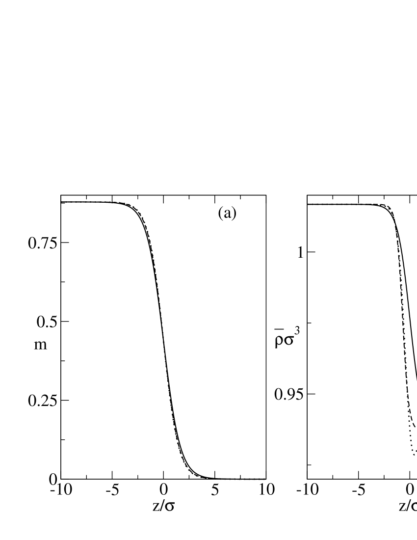
Figure 1: The crystallinity (a), and the average density (b), profiles as functions of position perpendicular to the interface as determined using the RLST DFT and parameterized profiles. Shown are results using hyperbolic tangent profiles with $B_{\rho}=B_{m}$ (solid lines), allowing $B_{\rho}\neq B_{m}$ (dashed lines), and with a Gaussian term in the density profile (dotted lines).

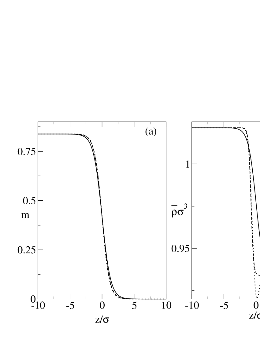
Figure 2: Same as Fig. 1 but using the White Bear DFT.

The structure of the liquid-solid interface is determined by minimizing the free energy functional, eq.(46), with respect to the spatially-dependent order parameters leading to the Euler-Lagrange equations

$$K_{ab}\left(\Gamma\left(u\right)\right)\frac{d^{2}}{du^{2}}\Gamma_{b}\left(u\right)+\left(\frac{\partial K_{ab}\left(\Gamma\left(u\right)\right)}{\partial\Gamma_{c}}-\frac{1}{2}\frac{\partial K_{bc}\left(\Gamma\left(u\right)\right)}{\partial\Gamma_{a}}\right)\frac{d\Gamma_{b}\left(u\right)}{du}\frac{d\Gamma_{c}\left(u\right)}{du}-\frac{\partial}{\partial\Gamma_{a}}\left(\frac{1}{V}\beta F\left(\Gamma\left(u\right)\right)-\beta\mu\overline{\rho}\right)=0$$ (48)

with

$$K_{ab}\left(\Gamma\right)=g_{ab}\left(\Gamma\left(u\right)\right)+2h_{ab}\left(\Gamma\left(u\right)\right)\left(\widehat{n}_{x}\widehat{n}_{y}+\widehat{n}_{x}\widehat{n}_{z}+\widehat{n}_{y}\widehat{n}_{z}\right)$$

and the boundary conditions

$$\lim_{u\rightarrow-\infty}\Gamma_{a} = \Gamma_{a}^{s}$$ (49)

$$\lim_{u\rightarrow-\infty}\Gamma_{a} = \Gamma_{a}^{l}$$

where $\Gamma^{s}=\left(m_{sol},\overline{\rho}_{sol}\right)$, etc. Direct solution of the Euler-Lagrange equations is difficult due to the presence of unstable solutions. So, in addition to this method (discussed below), parameterized forms of the order parameters were explored. Perhaps the most natural choice is to model the order parameters as simple hyperbolic tangents,

$$\Gamma_{a}(u)=\Gamma_{a}^{l}+\left(\Gamma_{a}^{s}-\Gamma_{a}^{l}\right)\frac{1}{2}\left(\tanh\left(A_{a}\left(u-B_{a}\right)\right)+1\right)$$ (50)

so that one minimizes the free energy with respect to the widths and positions of the interface. The surface tension (actually, the surface free-energy) is calculated as

$$\tau=\frac{1}{A}\left(\beta\Omega_{GL}^{(Planer)}\left[\Gamma\right]-\beta\Omega_{GL}^{bulk}\right)$$ (51)

where $\Omega_{GL}^{bulk}$ is the free energy of either bulk phase. The results are shown in Table 3. First, the simple hyperbolic tangent profiles with the interface fixed at $B_{m}=B_{\rho}=0$ gives surface tension of $0.73$ for RLST and $0.75$ for WB. Allowing the interfaces to move gives a relative displacement of nearly one hard-sphere diameter and lowers the surface tensions to $\allowbreak 0.67$ and $0.66$ respectively while giving a considerably narrower density profile. As a further refinement, inspired by the numerical results discussed below, a Gaussian term was added giving

$$\Gamma_{a}=\Gamma_{a}^{l}+\left(\Gamma_{a}^{s}-\Gamma_{a}^{l}\right)\frac{1}{2}\left(\tanh\left(A_{a}\left(u-B_{a}\right)\right)+1\right)+C_{a}\exp\left(-D_{a}\left(u-E_{a}\right)^{2}\right).$$ (52)

The addition of the Gaussian makes not appreciable difference for the profile of the crystallinity, but can affect the profile of the average density. The profiles of the order parameters are shown for the RLST and WB theories in Figs.(1) and (2) respectively. It is clear from the figures that there is little change in the profile of the crystallinity but the density is sensitive to functional forms used. These results were obtained using as initial values $A_{a}=0.5\sigma$, $B_{a}=C_{a}=E_{a}=0$ and $D_{a}=1$. Variation of the initial values by a factor of two has relatively little effect on the final result. However,. starting with much sharper widths, $A_{a}>2.5\sigma$, leads in some cases to a different minimum with a slightly lower surface tension and in other cases no minimum is found. It could be argued, however, that these cases are unphysical as the sharpness of the variation of the density violate the assumptions underlying the derivation of the Ginzburg-Landau form of the free energy (namely, that the order parameters vary slowly over atomic distances). The planer density profile, $\rho\left(u\right)=\frac{1}{A}\int\rho\left(\overrightarrow{r}\right)\delta\left(u-\overrightarrow{r}\cdot\widehat{n}\right)d\overrightarrow{r}$, corresponding to the RLST result using the combination of hyperbolic tangent and Gaussian is shown in Fig.(3)) for a profile in the [100] direction. It can be seen that in agreement with the results reported by Warshavsky and SongWarshavsky and Song (2006), the interface involves perhaps 8 lattice planes. The planer density corresponding to the offset hyperbolic tangents is indistinguishable from the one shown. In fact, from Figs. (1) and (2) it is clear that while all three profile functions give indistinguishable results for the crystallinity, the offset hyperbolic tangents and the hyperbolic tangent plus Gaussian give very similar profiles for the density and differ from the simple hyperbolic tangent profile. Furthermore, while in all cases one finds that going from the bulk liquid to the bulk solid, ordering (i.e. an increase in crystallinity) precedes densification (an increase in average density) due to the signficantly greater width of the crystallinity profile, the more complex parameterizations accentuate this by shifting the densification curve towards the bulk solid region.

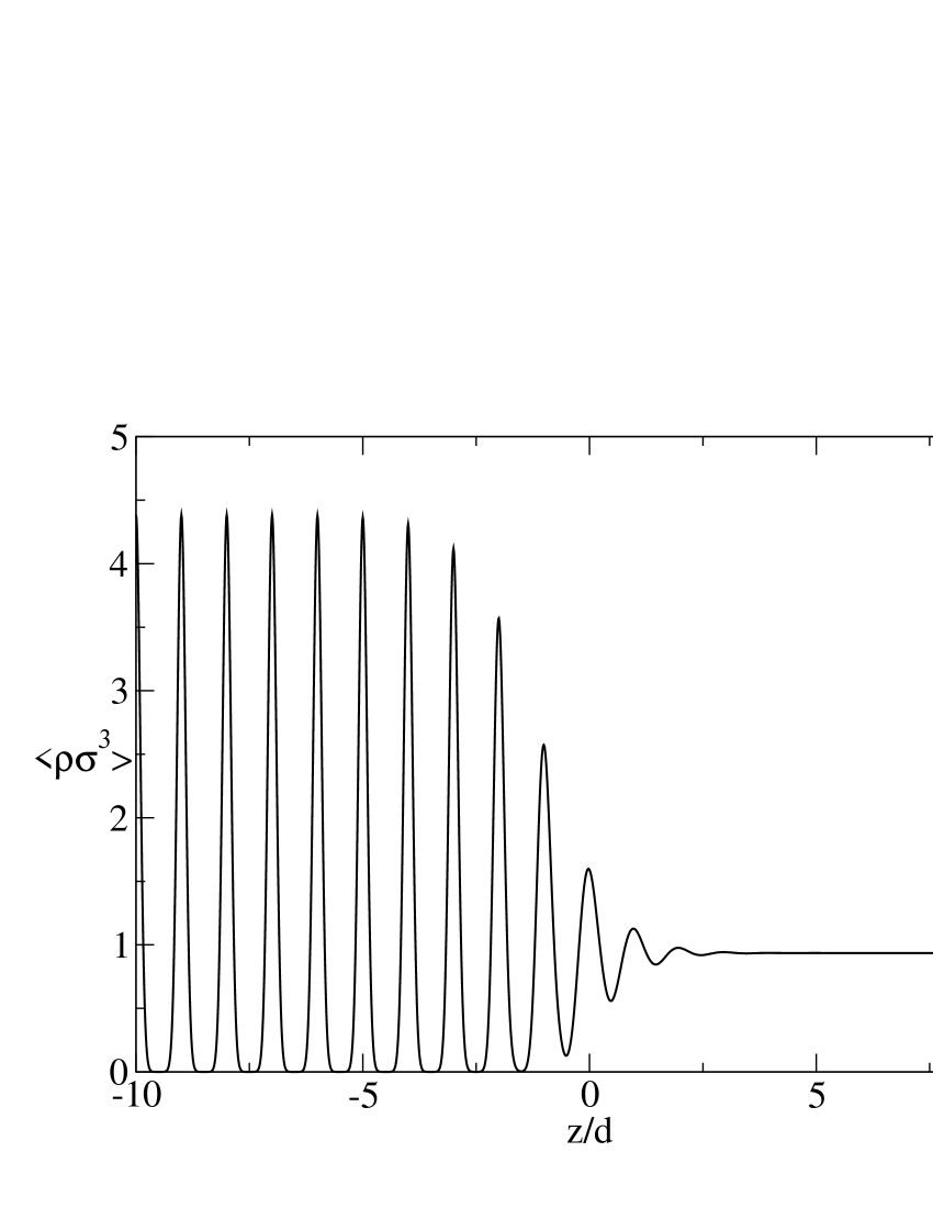
Figure 3: The atomic density averaged over planes perpendicular to the interface as a function of position, calculated using the RLST theory and the offset hyperbolic tangent parameterization. The position is shown in units of the interplaner spaceing for [100] planes, $d=0.5a$ where $a$ is the lattice parameter.

The direct integrations of the Euler-Lagrange equations is numerically challenging as there are both stable,physical solutions and unstable, unphysical solutions and the accumulation of numerical errors means that eventually all numerical integrations of the equations become unstable. To see this, note that far from the interfaces, one expects that the Euler-Lagrange equations can be linearized about the bulk values of the order parameters giving

$$\frac{d^{2}}{du^{2}}\delta\Gamma_{a}-K_{ab}^{-1}\left(\Gamma^{(0)}\right)\left[\frac{\partial^{2}}{\partial\Gamma_{b}\partial\Gamma_{c}}\frac{1}{V}\beta F\left(\Gamma\right)\right]_{\Gamma^{(0)}}\delta\Gamma_{c}=0$$ (53)

where $\Gamma_{a}^{(0)}$ are the bulk values of the order parameters and $\delta\Gamma_{a}=\Gamma_{a}-\Gamma_{a}^{(0)}$. The possible solutions are determined by the eigenvalues and eigenvectors of the matrix occurring in this equation. It turns out that in both the solid and liquid regions, there is one positive eigenvalue, allowing for decaying solutions, and one negative eigenvalue, corresponding to undamped oscillations. It is the mixing of the unphysical oscillatory solution with the decaying solution that causes numerical difficulties as illustrated in Fig. (4) for the RLST theory. The figure shows the result of integrating both from the bulk liquid towards the interface and from the bulk solid towards the interface with initial conditions chosen to allow for matching the solution at some point near the interface (thus constructing a shooting-method solution). Starting from the liquid, it is in fact possible to integrate almost completely through the interface until, in the solid region, pollution from the oscillatory solution causes the density to take on unphysical values. (Of course, unphysical values lie very close to the bulk value of the average density thus requiring relatively little inaccuracy to achieve this.) Note that the curve so obtained shows a slight depletion of the density near the interface as well as some structure on the solid side of the interface. Both of these effects are very small, given the overall small change in density between the liquid and solid, and are probably of little physical consequence. Integrating from the solid side shows similar effects as well as similar oscillations in the bulk liquid region. The surface tension of the shooting solution is $\gamma\sigma^{2}/k_{B}T\simeq 0.67$ which is not much different from that of the curve beginning from the liquid or solid sides which give $0.64$ and $0.65$ respectively. These figures are consistent with the surface tension obtained using the parameterized profiles and support the contention that the parameterizations are reasonably accurate.

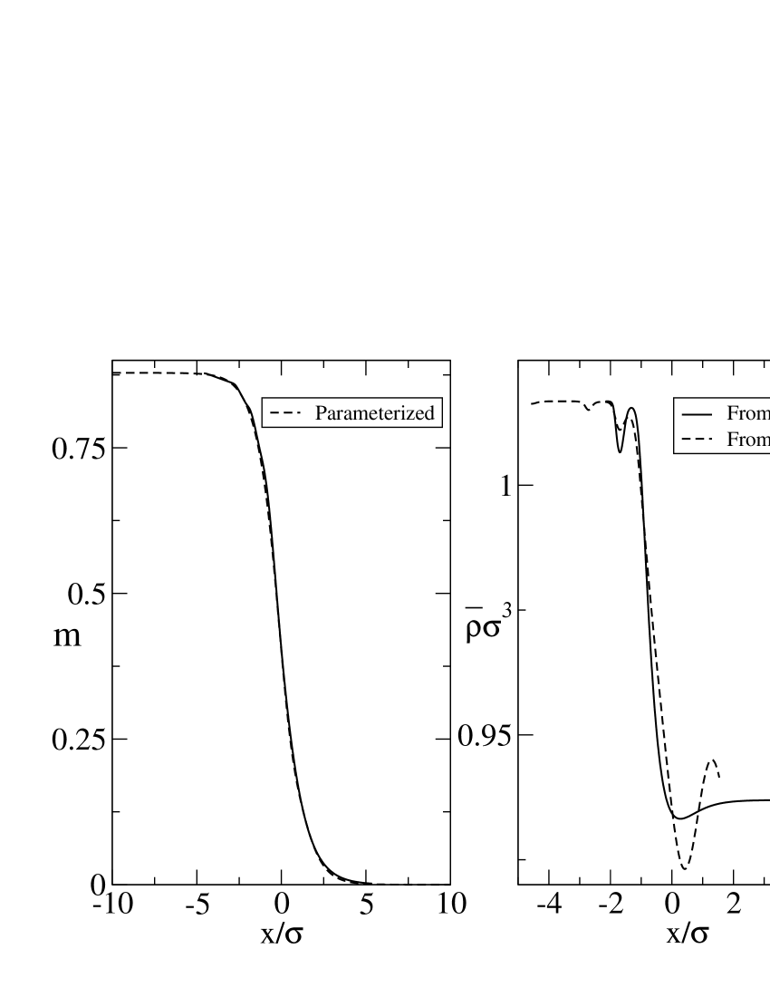
Figure 4: The crystallinity, left, and the average density, right, obtained by numerical integration of the Euler-Lagrange equations based on the RLST DFT. In the case of the crystallinity, the hyperbolic tangent profile discussed above is also shown. For the average density, the curves obtained by integrating from both the bulk solid and the bulk liquid regions is shown.

The surface tension of the planer interface has been determined from both Molecular Dynamics (MD)Davidchack and Laird (2000) and Monte Carlo (MC) simulationsMu et al. (2005). The MD gives values of $\gamma\sigma^{2}/k_{B}T=0.62,0.65$ and $0.58$ for the [100], [110] and [111] directions respectively while the MC gives $\gamma\sigma^{2}/k_{B}T=0.64,0.62$ and $0.61$. These results show a weak dependence on the orientation of the interface and the observed variation is not consistent between the two methods which perhaps indicates that the asymmetry is very small. The agreement between these values and those calculated from the GL model are therefore quite good. As expected, the WB model, which incorporates a better equation of state for the liquid than does the RLST model, seems to be slightly more accurate. The remaining differences between the calculations and the simulations can at least in part be attributed to the imposition of an invariant lattice structure.

Table 3: The order parameter profile parameters obtained by minimizing the free energy. The profiles studied are the hyperbolic tangents with $B_{m}=B_{\rho}$ (H), the “offset” hyperbolic tangents where $B_{m}\neq B_{rho}$ (OH), and the hyperbolic tangents with a Gaussian term (HG).Also included are the results from MD simulations of ref Davidchack and Laird (2000) and the MC simulations of ref.Mu et al. (2005) . In all cases, the last column gives the surface tension.

Theory	Profile	$A_{m}$	$A_{\rho}$	$B_{\rho}$	$C_{\rho}$	$D_{\rho}$	$E_{\rho}$	$\gamma\sigma^{2}/k_{B}T$
RLST	H	0.61	0.83	*	*	*	*	0.730
RLST	OH	0.67	1.64	-0.70	*	*	*	0.669
RLST	HG	0.68	0.99	*	-0.039	1.27	0.04	0.667
WB	H	0.74	0.84	*	*	*	*	0.754
WB	OH	0.85	2.54	-0.78	*	*	*	0.659
WB	HG	0.88	1.70	*	-0.06	1.97	-0.21	0.656
MD								0.617
MC								0.623

III.3 Solid Clusters

The GL theory can also be used to study the structure of solid clusters embedded in the liquid. For a spherically symmetric system, the grand potential becomes

$$\beta\Omega_{GL}^{(Spherical)}\left[\Gamma\right]=4\pi\int_{0}^{\infty}\;\left[\beta F\left(\Gamma\left(R\right)\right)-\beta\mu\overline{\rho}\left(R\right)+\frac{1}{2}g_{ab}\left(\Gamma\left(R\right)\right)\frac{d\Gamma_{a}\left(R\right)}{dR}\frac{d\Gamma_{b}\left(R\right)}{dR}\right]R^{2}dR$$ (54)

giving the Euler-Lagrange equations

$$g_{ab}\left(\Gamma\left(R\right)\right)R^{-2}\frac{d}{dR}R^{2}\frac{d\Gamma_{b}\left(R\right)}{dR}+\left(\frac{\partial g_{ab}\left(\Gamma\left(R\right)\right)}{\partial\Gamma_{c}\left(R\right)}-\frac{1}{2}\frac{\partial g_{bc}\left(\Gamma\left(R\right)\right)}{\partial\Gamma_{a}\left(R\right)}\right)\frac{d\Gamma_{b}\left(R\right)}{dR}\frac{d\Gamma_{c}\left(R\right)}{dR}-\frac{\partial}{\partial\Gamma_{a}\left(R\right)}\left(\beta F\left(\Gamma\left(R\right)\right)-\beta\mu\overline{\rho}\left(R\right)\right)=0.$$ (55)

The boundary conditions are

$$\lim_{R\rightarrow 0}\frac{d\Gamma_{a}\left(R\right)}{dR} = 0$$ (56)

$$\lim_{R\rightarrow\infty}\Gamma_{a}\left(R\right) = \Gamma_{a}^{l}\left(R\right)$$

Note that the first condition ensures that the first derivative along any line passing through the origin is continuous, e.g.

$$\lim_{x\uparrow 0}\frac{d\Gamma_{a}\left(R\right)}{dx}=\lim_{x\downarrow 0}\frac{d\Gamma_{a}\left(R\right)}{dx}.$$ (57)

Classical nucleation theory (CNT) is based on the observation that, to a first approximation, the excess free energy of a solid cluster of radius $R$ embedded in a large volume of fluid will be

$$\Delta\Omega^{cluster}\equiv\Omega^{cluster}\left[\Gamma\right]-\Omega^{liquid}\sim\frac{4\pi}{3}R^{3}\Delta\omega^{bulk}+4\pi R^{2}\gamma$$ (58)

where $\Delta\omega^{bulk}$ is the difference in the bulk solid and liquid free energies per unit volume. The stability of a cluster of a given radius clearly depends on the value of $\frac{\partial}{\partial R}\Delta\Omega^{cluster}$. If the liquid is the favored state, so that $\Omega_{GL}^{solid}>\Omega_{GL}^{liquid}$, then $\frac{\partial}{\partial R}\Delta\Omega^{cluster}>0$ for all $R$ meaning that any cluster will collapse to $R=0$. If the solid is favored, $\beta\Omega_{GL}^{solid}<\beta\Omega_{GL}^{liquid}$, clusters smaller than $R_{c}\simeq 2\gamma\left(\Delta\omega^{bulk}\right)^{-1}$ will collapse while those with $R>R_{c}$ will be unstable towards unlimited expansion. At this point, $\frac{\partial^{2}}{\partial R^{2}}\Delta\Omega^{cluster}=-8\pi\gamma<0$ so the critical cluster is a maximum in the free energy with

$$\Delta\Omega^{cluster}\left(R_{c}\right)\simeq\frac{16}{3}\pi\frac{\gamma^{3}}{\left(\Delta\omega^{bulk}\right)^{2}}.$$ (59)

This has been derived under the assumption that the surface tension is independent of $R$. In fact, as defined above, the surface tension only applies to conditions of coexistence so that for hard spheres it is a unique property. Another way of expressing this is that this classical nucleation model can only apply very close to coexistence. In that case, one can also write

$$\Delta\omega^{bulk} = \left(\frac{1}{V}F_{s}\left(\rho_{s}\right)-\mu\rho_{s}\right)-\left(\frac{1}{V}F_{l}\left(\rho_{l}\right)-\mu\rho_{l}\right)$$

$$\simeq \left(\frac{1}{V}F_{s}\left(\rho_{s}^{coex}\right)+\left(\rho_{s}-\rho_{s}^{coex}\right)\left(\frac{\partial\frac{1}{V}F_{s}\left(\rho\right)}{\partial\rho}\right)_{\rho_{s}^{coex}}-\mu\rho_{s}\right)$$

$$-\left(\frac{1}{V}F_{l}\left(\rho_{s}^{coex}\right)+\left(\rho_{l}-\rho_{s}^{coex}\right)\left(\frac{\partial\frac{1}{V}F_{l}\left(\rho\right)}{\partial\rho}\right)_{\rho_{l}^{coex}}-\mu\rho_{s}\right)$$

$$= \left(\frac{1}{V}F_{s}\left(\rho_{s}^{coex}\right)+\left(\rho_{s}-\rho_{s}^{coex}\right)\mu^{coex}-\mu\rho_{s}\right)-\left(\frac{1}{V}F_{l}\left(\rho_{l}^{coex}\right)+\left(\rho_{l}-\rho_{l}^{coex}\right)\mu^{coex}-\mu\rho_{l}\right)$$

$$= \left(-P^{coex}+\left(\mu^{coex}-\mu\right)\rho_{s}\right)-\left(-P^{coex}+\left(\mu^{coex}-\mu\right)\rho_{l}\right)$$

$$= \left(\rho_{s}-\rho_{l}\right)\left(\mu^{coex}-\mu\right)$$

giving the well-known expression

$$\Delta\Omega^{cluster}\left(R_{c}\right)\simeq\frac{16}{3}\pi\frac{\gamma^{3}}{\left(\rho_{s}-\rho_{l}\right)^{2}\left(\mu-\mu^{coex}\right)^{2}}.$$ (61)

As in the previous Section, a parametrized form for the order parameters is considered. It is again assumed that a hyperbolic tangent is a reasonable guess for the shape of the interface so, taking account of the boundary conditions suggests using

$$\Gamma_{a}\left(R\right) = \Gamma_{a}^{l}+\left(\Gamma_{a}\left(0\right)-\Gamma_{a}^{l}\right)\frac{1+b_{a}R}{1+\left(b_{a}R\right)^{2}}\frac{1-\tanh\left(A_{a}(R-R_{a})\right)}{1-\tanh\left(-A_{a}R_{a}\right)}$$

$$= \Gamma_{a}^{l}+\left(\Gamma_{a}\left(0\right)-\Gamma_{a}^{l}\right)\frac{1+b_{a}R}{1+\left(b_{a}R\right)^{2}}\left(\frac{1+\exp\left(-2A_{a}R_{a}\right)}{1+\exp\left(2A_{a}\left(R-R_{a}\right)\right)}\right)$$

with

$$b_{a}=\frac{2A_{a}}{e^{2A_{a}R_{a}}+1}.$$ (63)

This function has vanishing gradient at $R=0$ and for large $R$ decays as $\exp\left(-A_{a}R\right)/R$ which is the expected asymptotic formShiryayev and Gunton (2004). Note that the radius of the cluster is determined by $R_{\rho}$ and $R_{m}$which are of course not necessarily equal . For a fixed value of the chemical potential, $\mu$, the values of $\Gamma_{a}^{l}$ are computed from the known properties of the bulk liquid. Then, the profile is used in eq.(54) and the free energy minimized with respect to $\Gamma_{a}\left(0\right),A_{m},A_{\rho}$ and $R_{m}$ for a fixed value of $R_{\rho}$, which is taken to define the cluster size. In order to avoid unphysical regions, such as $m>1$, auxiliary variables $u$ and $v$ are defined via $\Gamma_{m}(0)=m_{max}\ast\frac{v^{2}}{1+v^{2}}$ and $\Gamma_{\rho}(0)=\rho_{max}-u^{2}$ where $m_{max}$ and $\rho_{max}$ are the maximum values occurring in the tables.

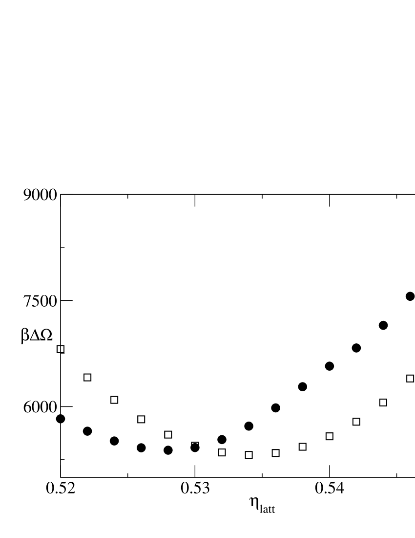
Figure 5: The excess free energy verses the lattice packing fraction, $\eta_{latt}=\pi\rho_{latt}\sigma^{3}/6$ for the RLST theory (filled symbols) and the WB theory (open symbols) for $R_{\rho}=30$ and $\beta\Delta\mu=0.25$

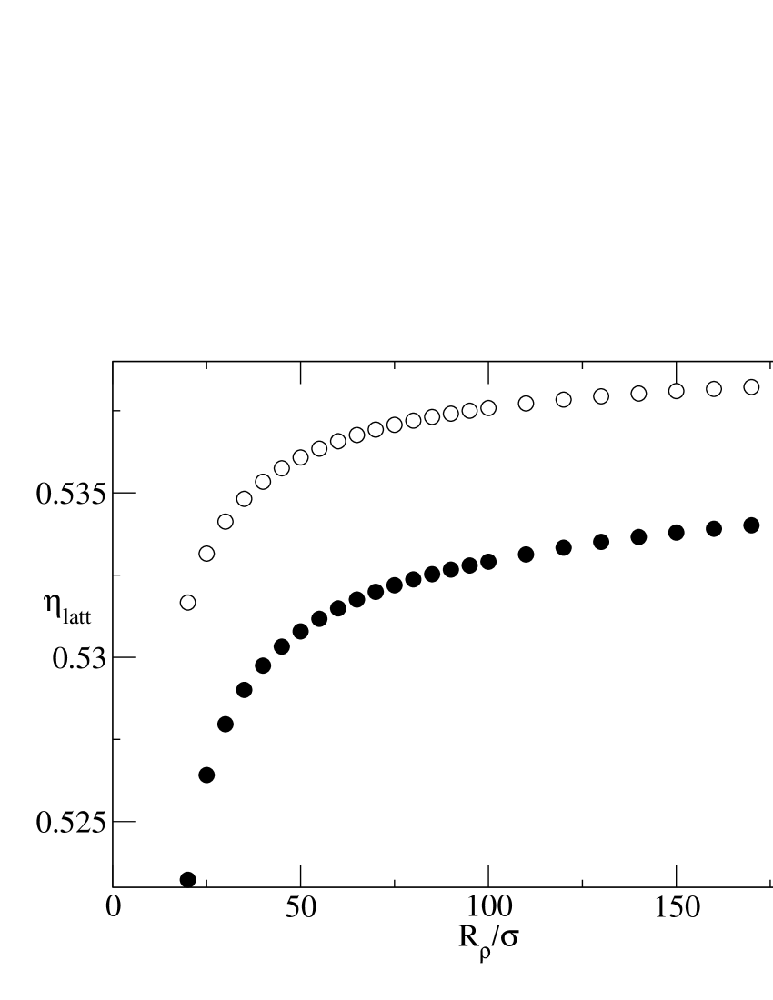
Figure 6: The lattice packing fraction, $\eta_{latt}=\pi\rho_{latt}\sigma^{3}/6$ as a function of the cluster size for the RLST theory (filled symbols) and the WB theory (open symbols)for $\beta\Delta\mu=0.25$

The critical cluster then corresponds to the value of $R_{\rho}$ for which the free energy is stationary. One difference from the planer interface is that the properties of the solid cluster cannot be assumed to be the same as those of a bulk solid with the specified chemical potential. Since the cluster is of finite size, the order parameters at the origin, $\Gamma_{a}\left(0\right)$, will in general differ from those of the bulk solid and, most importantly, the lattice parameter cannot be assumed to be that of the bulk solid. Thus, in addition to minimizing with respect to the parameters of the profile, it is also necessary to minimize with respect to the lattice parameter. These points are illustrated by Fig.5, showing the excess free energy as a function of the lattice density for particular values of the cluster radius and supersaturation. As expected, the excess free energy shows a minimum for a particular lattice density. Figure 6 shows the variation of the resulting lattice densities as a function of the radius of the cluster. For small clusters, the density is significantly lower than that of a bulk solid at the same chemical potential and increases rapidly as a function of cluster size. For larger clusters, the rate of change decreases as the bulk limit is approached although the variation with cluster size is still noticeable even for the largest clusters ($R_{1}=170\sigma$). The WB theory gives slightly higher densities than the RLST theory, as would be expected from the bulk coexistence data (see Table 1). In all cases, the average density at the core, $\bar{\rho}(0)$, is very close to the lattice density.

Figures 7(a) and 7(b) show the excess free energy as a function of the cluster size for different values of the supersaturation determined using the RLST and WB theories respectively. Also shown are the predicted excess free energy based on CNT, eq. (58), using the surface tension at coexistence obtained from the planer calculations of the previous Section. Clearly, CNT gives a reasonable approximation to the structure and energy of the critical cluster. In fact, this is a very sensitive test of the agreement between CNT and the detailed calculations. The largest discrepancy observed in the figures occurs for the lowest supersaturation, $\beta\Delta\mu=0.125$ and at largest cluster sizes. This is surprising since large clusters approach the bulk limit while surface tension becomes less important and one would expect that the CNT calculation would become increasingly accurate. However, since the radius of the critical cluster diverges as $\beta\Delta\mu\rightarrow 0$, the CNT results are very sensitive to the value of the chemical potential for small $\beta\Delta\mu$. This is illustrated in Fig. 7(b) where nearly perfect agreement between GL-DFT at $\beta\Delta\mu=0.125$ is found with the CNT result for $\beta\Delta\mu=0.120$ thus suggesting that the differences seen are at least in part due to numerical inaccuracies in the determination of the chemical potentials at coexistence. Other factors contributing to the disagreement are that the CNT assumes that the cluster has the properties of the bulk solid and that the surface tension is that for bulk coexisting ($\beta\Delta\mu=0$) phases.

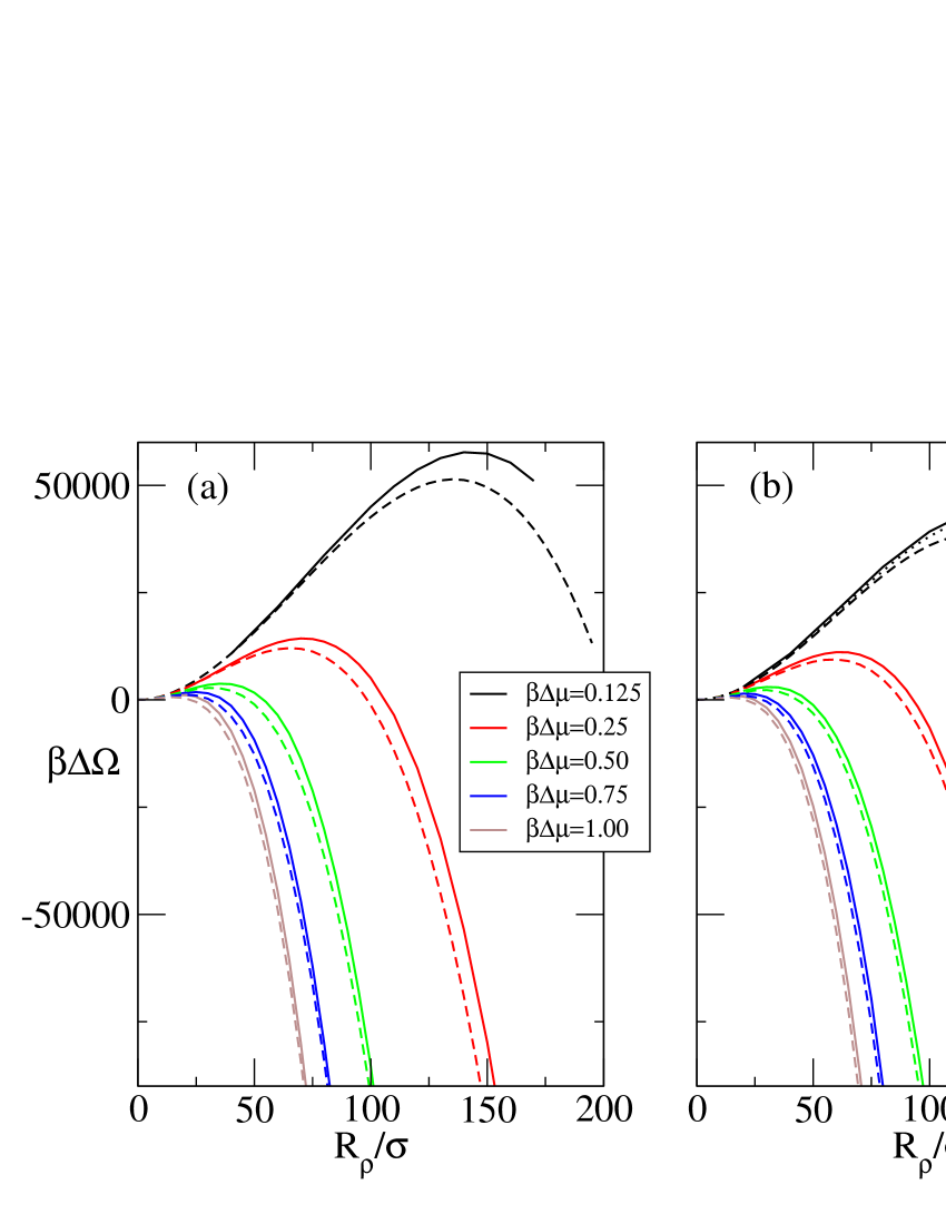
Figure 7: Excess free energy as a function of the cluster size as determined using (a) the RLST theory and (b) the WB theory. Curves are shown for $\beta\Delta\mu=0.125$, upper curves, to $\beta\Delta\mu=1.00$, lowest curves. The predicted excess free energies from CNT are also shown (broken lines).

Figure 8 shows that the lattice densities for small clusters are well below that of the bulk lattice density. A significant difference between the two DFT’s is apparent in that the RLST theory gives a discontinuity in the lattice density as a function of cluster size while the WB theory does not. The discontinuity arises because the free energy as a function of lattice density (for fixed cluster size and supersaturation) calculated using the RLST theory has two minima. For small clusters, the low-density minimum dominates while for larger clusters, the high-density minimum has lowest free energy. Further calculations have verified that for the lowest supersaturations shown in Fig. 8, the high-density minimum does dominate for sufficiently large clusters. Furthermore, the calculations also confirm that the high-density minimum is the one for which the density and crystallinity are closest to that of a bulk solid.

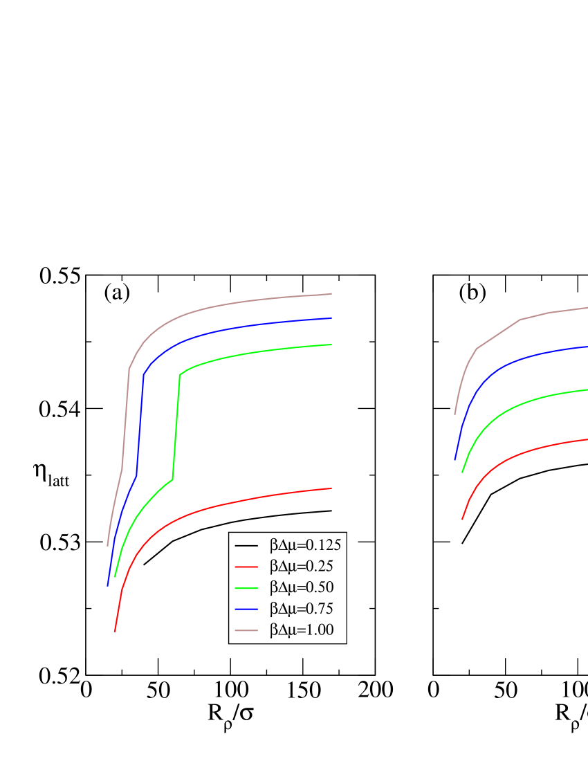
Figure 8: The lattice packing fraction as a function of the cluster size as determined using (a) the RLST theory and (b) the WB theory. Curves are shown for $\beta\Delta\mu=0.125$, upper curves, to $\beta\Delta\mu=1.00$, lowest curves.

Finally, in all cases, the structure of the liquid-solid interface is consistent with the results for the planer interface with similar values for the widths and relative displacements of the crystallinity and average density curves.

IV Conclusions

The primary results of this paper are the formulation of the Ginzburg-Landau free energy functional for hard-spheres based on Fundamental Measure Theory and the use of this functional to study the properties of the liquid-solid interface and of small FCC solid clusters in solution. It was shown that the required elements of the GL free energy functional can be calculated reasonably efficiently using FMT provided that the family of functionals of the density are extended. The resulting functional was used to study liquid-solid coexistence with a planer interface as well as the structure of small solid clusters.

For the planer interface between coexisting liquid and solid phases, the resulting surface tension is in reasonable agreement with simulation. No dependence of the surface tension on the lattice plane was found which is also consistent with simulation. Furthermore, the results using parameterized profiles and obtained via direct integration of the Euler-Lagrange equations were found to be consistent, notwithstanding the numerical difficulties of the latter procedure. This is an important point as, e.g., the early result obtained by Curtin using the WDA DFTCurtin (1989), which preceded determination of the surface tension for hard-spheres by computer simulation and seemed to be in good agreement with the later simulations, was subsequently shown by Ohnesorge et al.Ohnesorge et al. (1994) to be spurious and due, apparantly, to the use of over-constrained profiles. That same parameterization was also used by Marr and GastMarr and Gast (1993) and, with some modification, by Kyrlidis and BrownKyrlidis and Brown (1995). Recently, Warshavsky and Song, hereafter WS, performed similar calculations using FMT without the Ginzburg-Landau approximation. They observed greater differences from simulation than in the present work and non-negligable spatial asymmetry. The agreement between the present results and simulation may be fortuitous or the difference between the present results and those of WS may be due to other details in the later calculation such as the assumption of unit occupancy. In any case, the agreement between both FMT calculations and simulation is an improvement over the results based on older DFT’s which typically give a value of the planer surface tension that is about half of that measured in simulationOhnesorge et al. (1994); Marr and Gast (1993); Kyrlidis and Brown (1995).

The GL functional was also used to study the properties of small solid clusters in superdense solution. For the range of supersaturtions considered here, it was not found to be possible to stabilize clusters of radius less than about 15 hard-sphere radii; the free energy difference from the liquid is found to be very small and no local minimum in the free energy could be found. The results for clusters that could be stabilized are consistent with the predictions of classical nucleation theory. One interesting observation was that the RLST theory predicts a discontinuity in the structure of small clusters: very small clusters have unexpectedly low lattice densities while larger clusters approach the properties of the bulk solid. The crossover point between the two structures increases as the supersaturation increases and, conversely, appears to diverge near coexistence. However, since the RLST is based on a Percus-Yevik description of the fluid, which is not accurate at such high densities, and since the WB theory does not show this effect, it seems likely to be an artifact.

For both the planer interface and the clusters, it was found that moving from the bulk liquid towards the solid, one first observes ordering of the fluid and then densification. This is interesting as it is the opposite of the predictions of recent studies of crystallization directly from a low density gasLutsko and Nicolis (2006). For the latter case, it seems to always be more favorable to densify first, thus forming dense liquid droplets, and then to order. Of course, the main reason that this scenario is not observed here is that for hard-spheres it is only possible to study nucleation of the solid from an already-dense fluid - there is no equivalent of the low-density gas-solid transition. This is also undoubtedly one of the reasons that CNT seems to work so well for hard-spheres (i.e., because there is no critical point).

Although the Ginzburg-Landau model is reasonably successful in the applications described here, there are problems which cannot be discounted. Most important is that the free energy is unstable with respect to very sharp interfaces. Such rapid variations in the order parameters are outside the scope of the GL model, which is based on a gradient expansion, and so have been avoided here by always starting the minimizations from relatively slowly varying profiles. Within reasonable bounds for the starting parameters, the resulting profiles are then relatively insensitive to the starting point.

While of some intrinsic interest in testing the GL model and the density functional theory, these results are only intended as baselines for more interesting studies of realistic interaction models such as the Lennard-Jones potential. Since the only input to the GL model is a reasonable model for the bulk free energy and a reasonable model for the bulk direct correlation function, rather than a full blown density functional theory, it is expected that the extension of this work to other potentials will be relatively straightforward.

Appendix A Details of the calculations

A.1 The density functionals

All of the linear density functionals are of the form

$$n\left(\overrightarrow{r};\left[\rho\right]\right)=\int d\overrightarrow{r}_{1}\;w\left(\overrightarrow{r}-\overrightarrow{r}_{1}\right)\rho\left(\overrightarrow{r}_{1}\right).$$ (64)

As long as the density is written as a sum of basis functions at each lattice site,

$$\rho\left(\overrightarrow{r}\right)=\sum_{n}\overline{\rho}\left(\overrightarrow{r}-\overrightarrow{R}_{n}\right)$$ (65)

then the functionals can also be written as

$$n\left(\overrightarrow{r};\left[\rho\right]\right)=\sum_{n}\overline{n}\left(\overrightarrow{r}-\overrightarrow{R}_{n};\left[\rho\right]\right)$$ (66)

with

$$\overline{n}\left(\overrightarrow{r};\left[\rho\right]\right)=\int d\overrightarrow{r}_{1}\;w\left(\overrightarrow{r}-\overrightarrow{r}_{1}\right)\overline{\rho}\left(\overrightarrow{r}_{1}\right).$$ (67)

Before proceeding, note that in the case of tensorial quantities, $\overline{T}_{ij...k}\left(\overrightarrow{r};\left[\rho\right]\right)$, the only vector available is $\widehat{r}$ and the only tensor, aside from $\widehat{r}\widehat{r}$, is the unit tensor. Thus, it follows that

$$\overline{v}_{i}\left(\overrightarrow{r}\right) = v\left(r\right)\widehat{r}_{i}$$ (68)

$$\overline{T}_{ij}\left(\overrightarrow{r}\right) = A\left(r\right)\delta_{ij}+B\left(r\right)\widehat{r}_{i}\widehat{r}_{j}$$

$$\overline{T}_{ijl}\left(\overrightarrow{r}\right) = C(r)\left(\widehat{r}_{i}\delta_{jl}+\widehat{r}_{j}\delta_{il}+\widehat{r}_{l}\delta_{ij}\right)+D(r)\widehat{r}_{i}\widehat{r}_{j}\widehat{r}_{l}$$

$$\overline{T}_{ijlm}\left(\overrightarrow{r}\right) = E\left(r\right)\left(\delta_{ij}\delta_{lm}+\delta_{il}\delta_{jm}+\delta_{im}\delta_{jl}\right)$$

$$+F\left(r\right)\left(\widehat{r}_{i}\widehat{r}_{j}\delta_{lm}+\widehat{r}_{i}\widehat{r}_{l}\delta_{jm}+\widehat{r}_{i}\widehat{r}_{m}\delta_{jl}+\widehat{r}_{j}\widehat{r}_{l}\delta_{im}+\widehat{r}_{j}\widehat{r}_{m}\delta_{il}+\widehat{r}_{l}\widehat{r}_{m}\delta_{ij}\right)$$

$$+G\left(r\right)\widehat{r}_{i}\widehat{r}_{j}\widehat{r}_{l}\widehat{r}_{m}$$

The basic functionals for FMT are then found to be

$$\overline{s}\left(\overrightarrow{r}\right) = \frac{1}{2r}\sqrt{\frac{\alpha\sigma^{2}}{\pi}}\left(\exp\left(-\alpha\left(r-\frac{\sigma}{2}\right)^{2}\right)-\exp\left(-\alpha\left(r+\frac{\sigma}{2}\right)^{2}\right)\right)$$ (69)

$$\overline{\eta}\left(\overrightarrow{r}\right) = \frac{1}{2}\left(erf\left(\sqrt{\alpha}\left(r+\frac{\sigma}{2}\right)\right)\allowbreak-erf\left(\sqrt{\alpha}\left(r-\frac{\sigma}{2}\right)\right)\right)\allowbreak\allowbreak-\frac{1}{\alpha\sigma}\overline{s}\left(\overrightarrow{r}\right)$$

$$\overline{v}\left(\overrightarrow{r}\right) = \frac{1}{2r}\allowbreak\sqrt{\frac{\alpha\sigma^{2}}{\pi}}\left(\exp\left(-\alpha\left(r-\frac{\sigma}{2}\right)^{2}\right)+\exp\left(-\alpha\left(r+\frac{\sigma}{2}\right)^{2}\right)\right)-\frac{1}{\sigma\alpha r}\overline{s}\left(\overrightarrow{r}\right)$$

and the quantities needed for the tensorial functionals are

$$A\left(r\right) = \frac{1}{\sigma\alpha r}v\left(r\right)$$ (70)

$$B(r) = \overline{s}\left(r\right)-\frac{3}{\sigma\alpha r}v\left(r\right)\allowbreak$$

$$C\left(r\right) = \frac{1}{\alpha r\sigma}\allowbreak\allowbreak B\left(r\right)$$

$$D\left(r\right) = \overline{v}\left(r\right)-5C\allowbreak\left(r\right)$$

$$E\left(r\right) = \frac{1}{\alpha^{2}\sigma^{2}r^{2}}B\left(r\right)$$

$$F\left(r\right) = \frac{1}{\alpha r\sigma}\overline{v}\left(r\right)-5E\left(r\right)$$

$$G\left(r\right) = B\left(r\right)-7F\left(r\right)$$

Finally, one needs the additional quantities

$$\overline{\eta}^{i}\left(\overrightarrow{r}\right) = H\left(r\right)\widehat{r}_{i}$$ (71)

$$\overline{\eta}^{ij}\left(\overrightarrow{r}\right) = I\left(r\right)\widehat{r}_{i}\widehat{r}_{j}+J\left(r\right)\delta_{ij}$$

with

$$H\left(r\right) = \allowbreak r\overline{\eta}\left(r\right)-\frac{1}{2\alpha}\overline{v}\left(r\right)\allowbreak\allowbreak$$ (72)

$$I\left(r\right) = rH\left(r\right)-\frac{\sigma}{4\alpha}B(r)$$

$$J\left(r\right) = \frac{1}{2\alpha r}H\left(r\right).$$

In Fourier space one has that

$$n_{\alpha}\left(\overrightarrow{r};\left[\rho\right]\right) = \sum_{j}\rho_{j}\exp\left(i\overrightarrow{K}_{j}\cdot\overrightarrow{r}_{1}\right)\overline{n}_{\alpha}\left(\overrightarrow{K}_{j}\right)$$ (73)

$$\overline{n}_{\alpha}\left(\overrightarrow{K}\right) = \int d\overrightarrow{r}_{2}\;\exp\left(-i\overrightarrow{K}\cdot\overrightarrow{r}_{2}\right)w_{\alpha}\left(\overrightarrow{r}_{2}\right).$$

The tensorial quantities can be expressed as in real space but with the vector $\widehat{r}$ replaced by $\widehat{k}$ so

$$\overline{v}_{i}\left(\overrightarrow{K}\right) = v\left(r\right)\widehat{k}_{i}$$ (74)

$$\overline{T}_{ij}\left(\overrightarrow{K}\right) = A\left(k\right)\delta_{ij}+B\left(k\right)\widehat{k}_{i}\widehat{k}_{j}$$

$$\overline{T}_{ijl}\left(\overrightarrow{K}\right) = C(k)\left(\widehat{k}_{i}\delta_{jl}+\widehat{k}_{j}\delta_{il}+\widehat{k}_{l}\delta_{ij}\right)+D(k)\widehat{k}_{i}\widehat{k}_{j}\widehat{k}_{l}$$

$$\overline{T}_{ijlm}\left(\overrightarrow{K}\right) = E\left(k\right)\left(\delta_{ij}\delta_{lm}+\delta_{il}\delta_{jm}+\delta_{im}\delta_{jl}\right)$$

$$+F\left(k\right)\left(\widehat{k}_{i}\widehat{k}_{j}\delta_{lm}+\widehat{k}_{i}\widehat{k}_{l}\delta_{jm}+\widehat{k}_{i}\widehat{k}_{m}\delta_{jl}+\widehat{k}_{j}\widehat{k}_{l}\delta_{im}+\widehat{k}_{j}\widehat{k}_{m}\delta_{il}+\widehat{k}_{l}\widehat{k}_{m}\delta_{ij}\right)$$

$$+G\left(k\right)\widehat{k}_{i}\widehat{k}_{j}\widehat{k}_{l}\widehat{k}_{m}$$

The scalar and vector functionals are

$$\overline{s}\left(k\right) = \pi\sigma^{2}j_{0}\left(\frac{k\sigma}{2}\right)$$ (75)

$$\overline{\eta}\left(k\right) = \frac{1}{6}\pi\sigma^{3}\left(j_{0}\left(\frac{1}{2}k\sigma\right)+j_{2}\left(\frac{1}{2}k\sigma\right)\right)$$

$$\overline{v}_{a}\left(k\right) = -i\pi\sigma^{2}\frac{k_{a}}{k}j_{1}\left(\frac{k\sigma}{2}\right)$$

and the coefficients for the tensorial functionals are

$$A\left(k\right) = \frac{\pi\sigma^{2}}{3}\left(j_{0}\left(\frac{k\sigma}{2}\right)+j_{2}\left(\frac{k\sigma}{2}\right)\right)$$ (76)

$$B\left(k\right) = -\pi\sigma^{2}j_{2}\left(\frac{k\sigma}{2}\right)$$

$$C(k) = -i\frac{1}{5}\sigma^{2}\pi\left(j_{1}\left(\frac{k\sigma}{2}\right)+j_{3}\left(\frac{k\sigma}{2}\right)\right)$$

$$D(k) = i\sigma^{2}\pi j_{3}\left(\frac{k\sigma}{2}\right)$$

$$E\left(k\right) = \frac{1}{105}\sigma^{2}\pi\left(7j_{0}\left(\frac{k\sigma}{2}\right)+10j_{2}\left(\frac{k\sigma}{2}\right)+3j_{4}\left(\frac{k\sigma}{2}\right)\right)$$

$$F\left(k\right) = -\frac{1}{7}\sigma^{2}\pi\left(j_{2}\left(\frac{k\sigma}{2}\right)+j_{4}\left(\frac{k\sigma}{2}\right)\right)$$

$$G\left(k\right) = \sigma^{2}\pi j_{4}\left(\frac{k\sigma}{2}\right)$$

Finally,

$$\overline{\eta}^{i}\left(\overrightarrow{K}\right) = H\left(k\right)\widehat{k}_{i}$$ (77)

$$\overline{\eta}^{ij}\left(\overrightarrow{K}\right) = I\left(k\right)\widehat{k}_{i}\widehat{k}_{j}+J\left(k\right)\delta_{ij}$$

with

$$H\left(k\right) = i\frac{\sigma^{4}\pi}{20}\left(j_{1}\left(\frac{1}{2}k\sigma\right)+j_{3}\left(\frac{1}{2}k\sigma\right)\right)\allowbreak\allowbreak$$ (78)

$$I\left(k\right) = -\frac{\pi\sigma^{5}}{56}\left(j_{2}\left(\frac{1}{2}k\sigma\right)+j_{4}\left(\frac{1}{2}k\sigma\right)\right)$$

$$J\left(k\right) = \frac{\pi\sigma^{5}}{840}\left(7j_{0}\left(\frac{1}{2}k\sigma\right)+10j_{2}\left(\frac{1}{2}k\sigma\right)+3j_{4}\left(\frac{1}{2}k\sigma\right)\right).$$

A.2 The derivatives of the free energy

The free energy is written in terms of the integral of

$$\phi\left(\left\{n_{\alpha}\left(\overrightarrow{r}\right)\right\}\right)=\phi_{1}\left(\left\{n_{\alpha}\left(\overrightarrow{r}\right)\right\}\right)+\phi_{2}\left(\left\{n_{\alpha}\left(\overrightarrow{r}\right)\right\}\right)+\phi_{3}\left(\left\{n_{\alpha}\left(\overrightarrow{r}\right)\right\}\right)$$

and for the gradient term in the GL functional one needs the second derivatives of this function. Consider the first two terms which are the same for all of the DFTs,

$$\phi_{1}+\phi_{2}=-\frac{1}{\pi\sigma^{2}}s\ln\left(1-\eta\right)+\frac{1}{2\pi\sigma}\frac{s^{2}-v^{2}}{\left(1-\eta\right)}.$$ (79)

The second derivatives of these are

$$\frac{\partial^{2}}{\partial\eta^{2}}\left(\phi_{1}+\phi_{2}\right) = \frac{1}{\pi\sigma^{2}}\frac{s}{\left(1-\eta\right)^{2}}+\frac{1}{\pi\sigma}\frac{s^{2}-v^{2}}{\left(1-\eta\right)^{3}}$$ (80)

$$\frac{\partial^{2}}{\partial s^{2}}\left(\phi_{1}+\phi_{2}\right) = \frac{1}{\pi\sigma}\frac{1}{\left(1-\eta\right)}$$

$$\frac{\partial^{2}}{\partial v_{i}\partial v_{j}}\left(\phi_{1}+\phi_{2}\right) = \frac{1}{\pi\sigma}\frac{-1}{\left(1-\eta\right)}\delta_{ij}$$

and the cross-derivatives are

$$\frac{\partial^{2}}{\partial\eta\partial s}\left(\phi_{1}+\phi_{2}\right) = \frac{1}{\pi\sigma^{2}}\frac{1}{1-\eta}+\frac{1}{\pi\sigma}\frac{s}{\left(1-\eta\right)^{2}}$$ (81)

$$\frac{\partial^{2}}{\partial v_{i}\partial\eta}\left(\phi_{1}+\phi_{2}\right) = \frac{1}{\pi\sigma}\frac{-v_{i}}{\left(1-\eta\right)^{2}}$$

$$\frac{\partial^{2}}{\partial v_{i}\partial s}\left(\phi_{1}+\phi_{2}\right) = 0.$$

The third term takes different forms depending on the theory. For the RLST theory

$$\phi_{3}^{RLST}=\frac{1}{24\pi}\frac{s^{3}}{\left(1-\eta\right)^{2}}\left(1-\frac{v^{2}}{s^{2}}\right)^{3}$$ (82)

and the second derivatives are

$$\frac{\partial^{2}}{\partial\eta^{2}}\phi_{3}^{RLST} = \frac{1}{4\pi}\frac{s^{3}}{\left(1-\eta\right)^{4}}\left(1-\frac{v^{2}}{s^{2}}\right)^{3}$$ (83)

$$\frac{\partial^{2}}{\partial s^{2}}\phi_{3}^{RLST} = \frac{1}{4\pi}\frac{s}{\left(1-\eta\right)^{2}}\left(1-\frac{v^{2}}{s^{2}}\right)\left(1+\frac{v^{2}}{s^{2}}+2\left(\frac{v^{2}}{s^{2}}\right)^{2}\right)$$

$$\frac{\partial^{2}}{\partial v_{i}\partial v_{j}}\phi_{3}^{RLST} = \frac{1}{4\pi}\frac{s^{3}}{\left(1-\eta\right)^{2}}\left(1-\frac{v^{2}}{s^{2}}\right)\left(\frac{4v_{i}v_{j}+\delta_{ij}\left(v^{2}-s^{2}\right)}{s^{4}}\right)$$

and the cross derivatives are

$$\frac{\partial^{2}}{\partial\eta\partial s}\phi_{3}^{RLST} = \frac{1}{4\pi}\frac{s^{2}}{\left(1-\eta\right)^{3}}\left(1-\frac{v^{2}}{s^{2}}\right)^{2}\left(1+\frac{v^{2}}{s^{2}}\right)$$ (84)

$$\frac{\partial^{2}}{\partial\eta\partial v_{i}}\phi_{3}^{RLST} = -\frac{1}{2\pi}\frac{sv_{i}}{\left(1-\eta\right)^{3}}\left(1-\frac{v^{2}}{s^{2}}\right)^{2}$$

$$\frac{\partial^{2}}{\partial s\partial v_{i}}\phi_{3}^{RLST} = -\frac{1}{4\pi}\frac{v_{i}}{\left(1-\eta\right)^{2}}\left(1-\frac{v^{2}}{s^{2}}\right)\left(1+3\frac{v^{2}}{s^{2}}\right)$$

For the WB theory, first consider the simpler Tarazona theory which has

$$\phi_{3}^{T}=\frac{3}{16\pi}\frac{\overrightarrow{v}\cdot\overleftrightarrow{T}\cdot\overrightarrow{v}-sv^{2}-Tr\left(\overleftrightarrow{T}^{3}\right)+sTr\left(\overleftrightarrow{T}^{2}\right)}{\left(1-\eta\right)^{2}}$$ (85)

so

$$\frac{\partial^{2}}{\partial\eta^{2}}\phi_{3}^{T} = \frac{6}{\left(1-\eta\right)^{2}}\phi_{3}^{T}$$ (86)

$$\frac{\partial^{2}}{\partial s^{2}}\phi_{3}^{T} = 0$$

$$\frac{\partial^{2}}{\partial v_{i}\partial v_{j}}\phi_{3}^{T} = \frac{3}{16\pi}\frac{T_{ij}+T_{ji}-2s\delta_{ij}}{\left(1-\eta\right)^{2}}=\frac{3}{8\pi}\frac{T_{ij}-s\delta_{ij}}{\left(1-\eta\right)^{2}}$$

$$\frac{\partial^{2}}{\partial T_{ij}\partial T_{lm}}\phi_{3}^{T} = \frac{3}{16\pi}\frac{-3\delta_{jl}T_{mi}-3T_{jl}\delta_{il}+2s\delta_{lj}\delta_{mi}}{\left(1-\eta\right)^{2}}$$

and the cross-derivatives are

$$\frac{\partial^{2}}{\partial\eta\partial s}\phi_{3}^{T} = \frac{3}{8\pi}\frac{-v^{2}+Tr\left(\overleftrightarrow{T}^{2}\right)}{\left(1-\eta\right)^{3}}$$ (87)

$$\frac{\partial^{2}}{\partial\eta\partial v_{i}}\phi_{3}^{T} = \frac{3}{4\pi}\frac{T_{ia}v_{a}-sv_{i}}{\left(1-\eta\right)^{3}}=\frac{3}{4\pi}\frac{\left(T_{ia}-s\delta_{ia}\right)v_{a}}{\left(1-\eta\right)^{3}}$$

$$\frac{\partial^{2}}{\partial\eta\partial T_{ij}}\phi_{3}^{T} = \frac{v_{i}v_{j}-3T_{jc}T_{ci}+2sT_{ji}}{\left(1-\eta\right)^{3}}$$

$$\frac{\partial^{2}}{\partial s\partial v_{i}}\phi_{3}^{T} = -\frac{3}{8\pi}\frac{v_{i}}{\left(1-\eta\right)^{2}}$$

$$\frac{\partial^{2}}{\partial s\partial T_{ij}}\phi_{3}^{T} = \frac{3}{8\pi}\frac{T_{ji}}{\left(1-\eta\right)^{2}}$$

$$\frac{\partial^{2}}{\partial T_{ij}\partial v_{l}}\phi_{3}^{T} = \frac{3}{16\pi}\frac{\delta_{il}v_{j}+\delta_{jl}v_{i}}{\left(1-\eta\right)^{2}}$$

Now, in the WB theory one has

$$\phi_{3}^{WB} = F\left(\eta\right)\phi_{3}^{T}$$ (88)

$$F\left(\eta\right) = \frac{2}{3}\frac{\eta+\left(1-\eta\right)^{2}\ln\left(1-\eta\right)}{\eta^{2}}$$

$$F^{\prime}\left(\eta\right) = \frac{2}{3}\frac{\eta^{2}-2\eta-2\left(1-\eta\right)\ln\left(1-\eta\right)}{\eta^{3}}$$

$$F^{\prime\prime}\left(\eta\right) = \frac{2}{3}\frac{6\eta-\eta^{2}+\left(6-4\eta\right)\ln\left(1-\eta\right)}{\eta^{4}}$$

Then,

$$\frac{\partial^{2}}{\partial\Gamma_{a}\partial\Gamma_{b}}\phi_{3}^{WB} = F\left(\eta\right)\frac{\partial^{2}}{\partial\Gamma_{a}\partial\Gamma_{b}}\phi^{T}$$

$$+\delta_{b\eta}F^{\prime}\left(\eta\right)\frac{\partial}{\partial\Gamma_{a}}\phi^{T}+\delta_{a\eta}F^{\prime}\left(\eta\right)\frac{\partial}{\partial\Gamma_{b}}\phi^{T}$$

$$+\delta_{a\eta}\delta_{b\eta}F^{\prime\prime}\left(\eta\right)\phi^{T}$$

or

$$\frac{\partial^{2}}{\partial\Gamma_{a}\partial\Gamma_{b}}\phi_{3}^{WB}=\left(F\left(\eta\right)+\frac{1}{2}\left(1-\eta\right)\left(\delta_{a\eta}+\delta_{b\eta}\right)F^{\prime}\left(\eta\right)\right)\frac{\partial^{2}}{\partial\Gamma_{a}\partial\Gamma_{b}}\phi^{T}+\delta_{a\eta}\delta_{b\eta}F^{\prime\prime}\left(\eta\right)\phi^{T}$$ (90)

Appendix B Vanishing of $h_{ab}$ for the RLST theory

Combining eqs.(31) and (32) gives

$$h_{ab}\left(\Gamma\right)=-\frac{1}{4V}\sum_{\alpha,\beta}\int d\overrightarrow{r}_{1}d\overrightarrow{r}_{2}d\overrightarrow{r}\;\;r_{12x}r_{12y}\frac{\partial^{2}\phi\left(\left\{n_{\alpha}\left(\overrightarrow{r}\right)\right\}\right)}{\partial n_{\alpha}\partial n_{\beta}}w_{\alpha}\left(\overrightarrow{r}-\overrightarrow{r}_{1}\right)w_{\beta}\left(\overrightarrow{r}-\overrightarrow{r}_{2}\right)\frac{\partial\rho\left(\overrightarrow{r}_{1};\Gamma\right)}{\partial\Gamma_{a}}\frac{\partial\rho\left(\overrightarrow{r}_{2};\Gamma\right)}{\partial\Gamma_{b}}.$$ (91)

The goal here is to prove that this quantity vanishes in the RLST theory. The idea behind the proof is to make a change of variables in the integral whereby $\overrightarrow{r}_{i}=\left(x_{i},y_{i},z_{i}\right)\rightarrow\overrightarrow{r}_{i}^{\prime}=\left(-x_{i},y_{i},z_{i}\right)$ for $i=1,2$. This clearly gives an overall sign change as well as affecting the arguments of the various functions occurring under the integral. Using the fundamental fact that for a uniform solid (i.e. spatially constant $\Gamma$) with a cubic lattice structure, the density has reflection symmetry so that $\rho\left(\overrightarrow{r}_{i};\Gamma\right)=\rho\left(\overrightarrow{r}_{i}^{\prime};\Gamma\right)$ , it follows that the low order density functionals occurring in the RLST theory have simple parity and it is therefore possible to show that, aside from the overall change of sign, the integrand is invariant. This proves that $h_{ab}\left(\Gamma\right)=0$.

To begin,

$$h_{ab}\left(\Gamma\right) = -\frac{1}{4V}\sum_{\alpha,\beta}\int d\overrightarrow{r}_{1}d\overrightarrow{r}_{2}d\overrightarrow{r}\;\;x_{12}y_{12}\frac{\partial^{2}\phi\left(\left\{n_{\alpha}\left(\overrightarrow{r}\right)\right\}\right)}{\partial n_{\alpha}\partial n_{\beta}}w_{\alpha}\left(\overrightarrow{r}-\overrightarrow{r}_{1}\right)w_{\beta}\left(\overrightarrow{r}-\overrightarrow{r}_{2}\right)\frac{\partial\rho\left(\overrightarrow{r}_{1};\Gamma\right)}{\partial\Gamma_{a}}\frac{\partial\rho\left(\overrightarrow{r}_{2};\Gamma\right)}{\partial\Gamma_{b}}$$

$$= \frac{1}{4V}\sum_{\alpha,\beta}\int d\overrightarrow{r}_{1}^{\prime}d\overrightarrow{r}_{2}^{\prime}d\overrightarrow{r}\;\;x_{12}y_{12}\frac{\partial^{2}\phi\left(\left\{n_{\alpha}\left(\overrightarrow{r}\right)\right\}\right)}{\partial n_{\alpha}\partial n_{\beta}}w_{\alpha}\left(\overrightarrow{r}-\overrightarrow{r}_{1}^{\prime}\right)w_{\beta}\left(\overrightarrow{r}-\overrightarrow{r}_{2}^{\prime}\right)\frac{\partial\rho\left(\overrightarrow{r}_{1}^{\prime};\Gamma\right)}{\partial\Gamma_{a}}\frac{\partial\rho\left(\overrightarrow{r}_{2}^{\prime};\Gamma\right)}{\partial\Gamma_{b}}$$

$$= \frac{1}{4V}\sum_{\alpha,\beta}\int d\overrightarrow{r}_{1}^{\prime}d\overrightarrow{r}_{2}^{\prime}d\overrightarrow{r}^{\prime}\;\;x_{12}y_{12}\frac{\partial^{2}\phi\left(\left\{n_{\alpha}\left(\overrightarrow{r}^{\prime}\right)\right\}\right)}{\partial n_{\alpha}\partial n_{\beta}}w_{\alpha}\left(\overrightarrow{r}^{\prime}-\overrightarrow{r}_{1}^{\prime}\right)w_{\beta}\left(\overrightarrow{r}^{\prime}-\overrightarrow{r}_{2}^{\prime}\right)\frac{\partial\rho\left(\overrightarrow{r}_{1}^{\prime};\Gamma\right)}{\partial\Gamma_{a}}\frac{\partial\rho\left(\overrightarrow{r}_{2}^{\prime};\Gamma\right)}{\partial\Gamma_{b}}.$$

where we have also made the change of variable $\overrightarrow{r}=\left(x,y,z\right)\rightarrow\overrightarrow{r}^{\prime}=\left(-x,y,z\right)$. The claim is that $\Delta=0,$ where

$$\Delta = \sum_{\alpha,\beta}\Delta_{\alpha\beta}$$

$$\Delta_{\alpha\beta} = \frac{\partial^{2}\phi^{RLST}\left(\left\{n_{\alpha}\left(\overrightarrow{r}^{\prime}\right)\right\}\right)}{\partial n_{\alpha}\partial n_{\beta}}w_{\alpha}\left(\overrightarrow{r}^{\prime}-\overrightarrow{r}_{1}^{\prime}\right)w_{\beta}\left(\overrightarrow{r}^{\prime}-\overrightarrow{r}_{2}^{\prime}\right)$$

$$-\frac{\partial^{2}\phi^{RLST}\left(\left\{n_{\alpha}\left(\overrightarrow{r}\right)\right\}\right)}{\partial n_{\alpha}\partial n_{\beta}}w_{\alpha}\left(\overrightarrow{r}-\overrightarrow{r}_{1}\right)w_{\beta}\left(\overrightarrow{r}-\overrightarrow{r}_{2}\right)$$

Now, the scalar weight functions depend only on the magnitude of the separation, e.g. $w_{\eta}\left(\delta\overrightarrow{r}^{\prime}\right)=w_{\eta}\left(\left|\delta\overrightarrow{r}^{\prime}\right|\right)=w_{\eta}\left(\left|\delta\overrightarrow{r}\right|\right)$, so that they are invariant under the change of variables. The vector density $w_{\overrightarrow{v}}\left(\left|\delta\overrightarrow{r}^{\prime}\right|\right)=$ $\left(\delta\overrightarrow{r}^{\prime}/\left|\delta\overrightarrow{r}^{\prime}\right|\right)\Theta\left(\left|\delta\overrightarrow{r}^{\prime}\right|-\frac{\sigma}{2}\right)=$ $\left(\delta\overrightarrow{r}^{\prime}/\left|\delta\overrightarrow{r}\right|\right)\Theta\left(\left|\delta\overrightarrow{r}\right|-\frac{\sigma}{2}\right)$ so that $w_{v_{x}}\left(\left|\delta\overrightarrow{r}^{\prime}\right|\right)$ has odd parity and the other components have even parity. From this and the reflection symmetry of $\rho\left(\overrightarrow{r};\Gamma\right)$, it follows that the density functionals $\eta\left(\overrightarrow{r}\right)$ , $s\left(\overrightarrow{r}\right)$ and $\overrightarrow{v}\left(\overrightarrow{r}\right)$ have the corresponding parities (that is , all are even except $v_{x}\left(\overrightarrow{r}^{\prime}\right)=-v_{x}\left(\overrightarrow{r}\right)$). From the explicit expressions for $\frac{\partial^{2}\phi^{RLST}}{\partial n_{\alpha}\partial n_{\beta}}$ given in the previous appendix, it is seen that all of these have even parity except for those in which one and only one of the derivatives is with respect to $v_{x}\left(\overrightarrow{r}\right)$. It immediately follows that

$$\Delta_{ss}=\Delta_{\eta\eta}=\Delta_{s\eta}=\Delta_{\eta s}=\Delta_{v_{x}v_{x}}=\Delta_{v_{y}v_{y}}=\Delta_{v_{z}v_{z}}=\Delta_{v_{y}v_{z}}=0.$$

Finally, $\frac{\partial^{2}\phi^{RLST}}{\partial s\partial v_{x}},$ $\frac{\partial^{2}\phi^{RLST}}{\partial\eta\partial v_{x}},\frac{\partial^{2}\phi^{RLST}}{\partial v_{x}\partial v_{y}}$ and $\frac{\partial^{2}\phi^{RLST}}{\partial v_{x}\partial v_{z}}$ are all of odd parity (because they are proportional to $v_{x}$) as are $w_{s}w_{v_{x}},w_{\eta}w_{v_{x}},w_{v_{x}}w_{v_{y}}$ and $w_{v_{x}}w_{v_{z}}$ so that $\Delta_{sv_{x}}=\Delta_{\eta v_{x}}=\Delta_{v_{z}v_{y}}=\Delta_{v_{z}v_{z}}=0$ thus proving that $\Delta=0$ and hence that $h_{ab}\left(\Gamma\right)=0$ in the RLST theory. The same is not true of the WB theory as terms such as $T_{jc}T_{ci}$, and therefore

$$\frac{\partial^{2}}{\partial\eta\partial T_{ij}}\phi_{3}^{T}=\frac{v_{i}v_{j}-3T_{jc}T_{ci}+2sT_{ji}}{\left(1-\eta\right)^{3}},$$

do not have a definite parity under reflection.

References

- Evans (1979) R. Evans, Adv. Phys. 28, 143 (1979).
- Hansen and McDonald (1986) J.-P. Hansen and I. McDonald, Theory of Simple Liquids (Academic Press, San Diego, Ca, 1986).
- Haymet and Oxtoby (1981) A. D. J. Haymet and D. W. Oxtoby, J. Chem. Phys. 74, 2559 (1981).
- Oxtoby and Haymet (1982) D. W. Oxtoby and A. D. J. Haymet, J. Chem. Phys. 76, 6262 (1982).
- Curtin and Ashcroft (1986) W. A. Curtin and N. W. Ashcroft, Phys. Rev. Lett. 56, 2775 (1986).
- Ohnesorge et al. (1991) R. Ohnesorge, H. Lowen, and H. Wagner, Phys. Rev. A 43, 2870 (1991).
- Curtin (1989) W. A. Curtin, Phys. Rev. B 39, 6775 (1989).
- Marr and Gast (1993) D. W. Marr and A. P. Gast, Phys. Rev. E 47, 1212 (1993).
- Ohnesorge et al. (1994) R. Ohnesorge, H. Löwen, and H. Wagner, Phys. Rev. E 50, 4801 (1994).
- Rosenfeld (1989) Y. Rosenfeld, Phys. Rev. Lett. 63, 980 (1989).
- Rosenfeld et al. (1990) Y. Rosenfeld, D. Levesque, and J.-J. Weis, J. Chem. Phys. 92, 6818 (1990).
- Rosenfeld et al. (1997) Y. Rosenfeld, M. Schmidt, H. Löwen, , and P. Tarazona, Phys. Rev. E 55, 4345 (1997).
- Warshavsky and Song (2006) V. B. Warshavsky and X. Song, Phys. Rev. E 73, 031110 (2006).
- Lutsko (2006) J. F. Lutsko (2006), to appear in Physica A, URL http://arxiv.org/abs/cond-mat/0508363.
- Tarazona and Rosenfeld (1997) P. Tarazona and Y. Rosenfeld, Phys. Rev. E 55, 0R4873 (1997).
- Tarazona (2000) P. Tarazona, Phys. Rev. Lett. 84, 694 (2000).
- Tarazona (2002) P. Tarazona, Physica A 306, 243 (2002).
- Roth et al. (2002) R. Roth, R. Evans, A. Lang, and G. Kahl, J. Phys.: Cond. Matt. 14, 12063 (2002).
- Löwen et al. (1989) H. Löwen, T. Beier, and H. Wagner, Europhys. Lett. 9, 791 (1989).
- Löwen et al. (1990) H. Löwen, T. Beier, and H. Wagner, Z. Phys. B 79, 109 (1990).
- Groh and Mulder (2000) B. Groh and B. Mulder, Phys. Rev. E 61, 3811 (2000).
- Press et al. (1993) W. H. Press, S. A. Teukolsky, W. T. Vetterling, and B. P. Flannery, Numerical Recipes in C (Claredon Press, Oxford, 1993).
- (23) The gnu scientific library, eprint http://sources.redhat.com/gsl.
- Hoover and Ree (1968) W. G. Hoover and F. H. Ree, J. Chem. Phys. 49, 3609 (1968).
- Shiryayev and Gunton (2004) A. Shiryayev and J. D. Gunton, J. Chem. Phys. 120, 8318 (2004).
- Groh (2000) B. Groh, Phys. Rev. E 61, 5218 (2000).
- Davidchack and Laird (2000) R. L. Davidchack and B. B. Laird, Phys. Rev. Lett. 85, 4751 (2000).
- Mu et al. (2005) Y. Mu, A. Houk, and X. Song, J. Phys. Chem. B 109, 6500 (2005).
- Kyrlidis and Brown (1995) A. Kyrlidis and R. A. Brown, Phys. Rev. E 51, 5832 (1995).
- Lutsko and Nicolis (2006) J. F. Lutsko and G. Nicolis, Phys. Rev. Lett. 96, 046102 (2006), also appeared in February 15, 2006 issue of Virtual Journal of Biological Physics Research., eprint cond-mat/0510021, URL http://link.aps.org/abstract/PRL/v96/e046102.