Selective transmission of Dirac electrons and ballistic magnetoresistance of n-p junctions in graphene.

Abstract

We show that an electrostatically created n-p junction separating the electron and hole gas regions in a graphene monolayer transmits only those quasiparticles that approach it almost perpendicularly to the n-p interface. Such a selective transmission of carriers by a single n-p junction would manifest itself in non-local magnetoresistance effect in arrays of such junctions and determines the unusual Fano factor in the current noise universal for the n-p junctions in graphene.

The chiral nature of quasiparticles in graphene monolayers and bilayers Haldane ; DiVincenzo ; Semenoff ; DresselhausBook ; AndoNoBS ; McCann has been revealed in several recent experiments novo04 ; novo05 ; novo05pnas ; zhang05 ; NovoselovMcCann . The Fermi level in a neutral graphene sheet (a monolayer of carbon atoms with hexagonal lattice structure) is pinned near the corners of the hexagonal Brillouin zone kpoints which determine two non-equivalent valleys in the quasiparticle spectrum.  The quasiparticles in each of the two valleys are described by the Hamiltonian DresselhausBook ; Semenoff ,

$$\hat{H}_{1}=v\,\mathbf{\sigma}\cdot\mathbf{p},$$

where the ’isospin’ Pauli matrices $\sigma_{i}$ operate in the space of the electron amplitude on two sites (A and B) in the unit cell of a hexagonal crystal kpoints , $\mathbf{p}=(p_{x},p_{y})=-i\mathbf{\nabla}$ is the momentum operator hbar1 defined with respect to the centre of the corresponding valley, and $v$ is a constant formed by the A-B hopping DresselhausBook . The Dirac-type Hamiltonian $\hat{H}_{1}$ determines the linear dispersion $vp$ for the electron, and $-vp$ for the hole branch of quasiparticles. In each valley kpoints , the electron and hole states also differ by the isospin projection onto the direction of their momentum: electrons have chirality $\mathbf{\sigma}\cdot\mathbf{p}/p=1$, holes $\mathbf{\sigma}\cdot\mathbf{p}/p=-1$. Therefore, in structures where the quasiparticle isospin is conserved (, a monolayer with electrostatic potential scattering) their backscattering is strictly forbidden AndoNoBS , which gives rise to the peculiar properties of the n-p junction in graphene reported in this Letter.

Since an atomically-thin graphitic film is a gapless semiconductor, carrier density in it can be varied using external gates novo04 from electrons to holes novo04 ; novo05 ; novo05pnas ; zhang05 ; NovoselovMcCann . A planar n-p junction in graphene can be made, e.g., using split-gates, and in view of a rapidly improving mobility of the new material novo05 ; novo05pnas ; zhang05 it may soon be possible to fabricate ballistic circuits of electrically controlled graphene-based n-p junctions. Below, we model the n-p junction in graphene using the electrostatic potential $u(x)=vk_{F}\eta(x/d)$ characterized by a single length scale $d$ and the Fermi momentum $k_{F}$ determined by the equal densities of the electron and hole gases on the opposite sides of it. Here $\eta(\pm\infty)=\pm 1$, $\eta^{\prime}(0)=1$, and the line $x=0$ separates the p- and n-regions. Since in a junction produced by electrostatic gates the length $d$  is about the inter-gate distance and exceeds the electron wavelength in a monolayer, we focus this study on smooth n-p junctions with $k_{F}d>1$, and show that their transmission properties are determined by the central region where $u(x)\approx Fx$ [$F=vk_{F}/d$].

The transport properties of the n-p junction are determined by the angular dependence of the probability $w(\theta)$ of an electron incident from the left with an energy equal to the chemical potential $\mu=0$ to emerge as a hole on the right hand side of the junction. The electron approaching the center of the junction has the kinetic energy $v\sqrt{p_{x}^{2}+p_{y}^{2}}$, where $p_{y}=k_{F}\sin\theta$ is conserved. Due to the energy conservation, the $x$-component of the electron momentum is $p_{x}(x)=\sqrt{u^{2}(x)/v^{2}-p_{y}^{2}}$, the classically allowed region for the electron motion is determined by the condition $|u|>p_{y}v$ and its trajectory cannot extend beyond the turning point at the distance $l=vp_{y}/F$ from the center of the junction footnote-momentum . For a particle incident perpendicular to the junction ($p_{y}=0$) the classically forbidden region disappears. Moreover, due to the isospin conservation which prohibits backscattering of chiral quasiparticles AndoNoBS , the wave incident at $\theta=0$ is perfectly transmitted, though, for any small $\theta$, the transmission probability is determined by tunnelling through the classically forbidden region, $w\sim e^{-2S}$, where $S=i\int_{-l}^{l}p_{x}(x)dx=\frac{1}{2}\pi vp_{y}^{2}/F$. For a smooth n-p junction shown in Fig. 1 with $F=vk_{F}/d$ and $k_{F}d\gg 1$, this yields (for $\theta\ll\pi/2$)

$$w(\theta)=e^{-\pi(k_{F}d)\sin^{2}\theta}.$$ (1)

The angular dependence of the transmission probability given in Eq. (1) is, in fact, exact in the range $\theta\ll\pi/2$ for any smooth junction and represents the central result of this Letter. Below, we rigorously derive the result in Eq. (1) using the method of transfer matrix and also show that $w(\theta)=\cos^{2}\theta$ for a step-like potential. Similarly to the formulae Glazman describing adiabatic ballistic constrictions in semiconductors, the applicability of Eq. (1) is not restricted by the constraint $w\ll 1$. This can be used to describe how a smooth n-p junction selectively transmits only carriers approaching it within a small angle $\theta\lesssim\theta_{0}=1/\sqrt{\pi k_{F}d}$ around the perpendicular direction and to determine the conductance per unit length of a broad junction,

$$g_{np}=\frac{4e^{2}}{h}\int\frac{k_{F}d\theta}{2\pi}w(\theta)\approx\frac{2e^{2}}{\pi h}\sqrt{\frac{k_{F}}{d}},$$ (2)

and the universal Fano factor footnoteBeen in the shot noise,

$$\langle\langle I\cdot I\rangle\rangle=(1-\sqrt{\tfrac{1}{2}})\,eI.$$ (3)

At the end of this paper we shall discuss several ballistic magnetoresistance effects which exploit the selectivity of transmission implicit in Eq. (1).

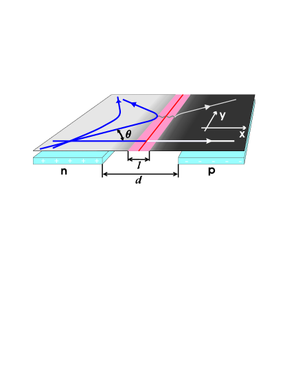
Figure 1: Angular dependence of quasiparticle transmission through the electrostatically generated n-p junction in graphene.

To formulate the scattering problem, we shall exploit the separation of $x$ and $y$ variables for the electron motion across the junction (in $x$ direction) and the fact that momentum along $y$-axis (parallel to the junction) is conserved. This makes the scattering problem one-dimensional (1D). The scattering states at the energy equal to the chemical potential, $\mu=0$ are spinors satisfying the Dirac-type equation

$$-i\partial_{x}\sigma_{x}\psi+v^{-1}u(x)\psi+p_{y}\sigma_{y}\psi=0,$$ (4)

which conserves the 1D current $J_{x}=\psi^{\dagger}\sigma_{x}\psi$.

To find the transmission probability $w(\theta)$ for such states, we calculate the transfer matrix $T(x,y)$ which satisfies the equation

$$\partial_{x}T(x,y)=L(x)\,T(x,y),\;L=-i\frac{u(x)}{v}\sigma_{x}+p_{y}\sigma_{z}$$ (5)

and the conditions $T(y,y)=I,$ $T(x,y)=T(x,z)T(z,y),$ $\det T(x,y)=1,$ and $T^{\dagger}(x,y)\sigma_{x}T(x,y)=\sigma_{x}$. To relate the transmission coefficient $w$ to the transfer matrix $T(x,y)$ one has to factor out the asymptotic evolution of the reflected and transmitted waves. This can be done by using matrices $A_{\pm}$ satisfying the wave equation in the asymptotic regions,

$$\partial_{x}A_{\pm}(x)=(\mp ik_{F}\sigma_{x}+p_{y}\sigma_{z})A_{\pm}(x),$$ (6)

such that their columns are made of right- and left-propagating states normalized to carry unit current. The explicit expression for these matrices is

$$A_{\pm}(x)=\sqrt{\frac{k_{F}}{2p_{x}}}\left(\begin{array}[]{ll}\frac{p_{x}\pm ip_{y}}{k_{F}}e^{\mp ip_{x}x}&\frac{-p_{x}\pm ip_{y}}{k_{F}}e^{\pm ip_{x}x}\\ e^{\mp ip_{x}x}&e^{\pm ip_{x}x}\end{array}\right),$$

where $p_{x}(x)=\sqrt{u^{2}(x)/v^{2}-p_{y}^{2}}=\sqrt{k_{F}^{2}-p_{y}^{2}}.$ Then, the transmission probability can be found using the matrix

$$\left(\begin{array}[]{cc}\alpha&\beta^{\ast}\\ \beta&\alpha^{\ast}\end{array}\right)\equiv\lim_{x\rightarrow\infty}A_{+}^{-1}(x)T(x,-x)A_{-}(-x),\;\;w=\frac{1}{|\alpha|^{2}}.$$ (7)

To illustrate the transfer matrix formalism, we calculate the probability of a Dirac fermion transmission through a sharp potential step $u(x)=vk_{F}\mathrm{sign}(x).$ In this case, we factor the transfer matrix as $T(x,y)=T_{+}(x,0)T_{-}(0,y)$, where $T_{+(-)}(x,y)$ is a transfer matrix on the right(left) side of the junction, each given by $T_{\pm}(x,y)=A_{\pm}(x)A_{\pm}^{-1}(y)$. Using this solution and Eq. (7) we find

$$\left(\begin{array}[]{cc}\alpha&\beta^{\ast}\\ \beta&\alpha^{\ast}\end{array}\right)=A_{+}^{-1}(0)A_{-}(0),\;\alpha=1-\frac{ip_{y}}{\sqrt{k_{F}^{2}-p_{y}^{2}}}.$$

For the transmission probability this yields

$$w=1-(p_{y}/k_{F})^{2}=\cos^{2}\theta,$$ (8)

which manifests the chiral nature of quasiparticles in graphene. Indeed, the free electron states of the Dirac Hamiltonian $\hat{H}_{1}$ have their isospin polarized along the momentum (for the transmitted holes, with $\mathbf{p}=(-k_{F}\cos\theta,k_{F}\sin\theta)$, it is antiparallel), and the reflection amplitude of an electron is determined by the scalar product $\psi_{\nearrow}^{\dagger}\cdot\psi_{\nwarrow}\sim\sin\theta$ of its initial and final state spinors.

To calculate the transmission probability for a smooth potential with $k_{F}d\gg 1$, we separate the $x$-axis across the junction into the inner (i) and outer (o) parts. In the outer part, $\left|x\right|>cd$ (where $c\ll 1$), we find the T-matrix, $T_{o}$ using the method of adiabatic expansion. Then, we match it with the exact solution, $T_{i}$ obtained in the central part of the junction, $\left|x\right|<d$, where the potential $u(x)$ can be linearised, $u(x)\approx{k_{F}x}/{d}$, and obtain the complete tranfer matrix as $T(y,x)=T_{o}(x,a)T_{i}(a,-a)T_{o}(-a,y)$.

For the adiabatic expansion of the transfer matrix $T_{o}$ we use a transformation

$$Y(x)=\frac{1}{u}\left(\begin{array}[]{ll}i\varkappa&i\varkappa^{\ast}\\ u&u\end{array}\right),\;\left\{\begin{array}[]{c}p_{x}(x)=\sqrt{\dfrac{u^{2}}{v^{2}}-p_{y}^{2}},\\ \varkappa=p_{y}+ip_{x}(x).\end{array}\right.$$ (9)

which locally diagonalises the $L$ operator in Eq. (5):

$$Y^{-1}LY=ip_{x}(x)\sigma_{z}.$$ (10)

The transfer matrix $\tilde{T}_{o}$ defined in a new basis,

$$T_{o}(x,y)=Y(x)\tilde{T}_{o}(x,y)Y^{-1}(y),$$ (11)

satisfies the equation

$$\partial_{x}\tilde{T}_{o}(x,y)=ip_{x}(x)\sigma_{z}\tilde{T}_{o}(x,y)+\Omega(x)\tilde{T}_{o}(x,y),$$ (12)

$$Q=-Y^{-1}\partial_{x}Y=\frac{p_{y}u^{\prime}(x)}{2p_{x}^{2}(x)u(x)}\left(\begin{array}[]{ll}-\varkappa&\varkappa^{\ast}\\ \varkappa&-\varkappa^{\ast}\end{array}\right).$$ (15)

In the adiabatic approximation the matrix $\Omega(x)$ is assumed to be small as compared to the diagonal term $p_{x}(x)\sigma_{z}$, and to the leading order Eq. (12) is solved by

$$\tilde{T}_{o}(x,y)=\exp\left[i\sigma_{z}\int_{y}^{x}p_{x}(x^{\prime})dx^{\prime}\right].$$ (16)

Formally, the adiabatic approximation is justified if $\left|p_{y}u^{\prime}/(up_{x}^{2})\right|\ll 1$, which breaks down near the turning points $p_{x}(x)=0$ and when $u(x)=0$. However, for the junctions with $k_{F}d\gg 1$, the interval between turning points lies within the region of space where the the potential profile can be approximated using the linear function $u(x)={k_{F}x}/{d}$. The transfer matrix in this region, $T_{i}$ can be found from Eq. (5) exactly, using the transformation

$$T_{i}(x,y)=e^{-i\frac{\pi}{4}\sigma_{y}}e^{-i\frac{\phi(x)}{2}\sigma_{z}}\tilde{T}_{i}(x,y)e^{i\frac{\phi(y)}{2}\sigma_{z}}e^{i\frac{\pi}{4}\sigma_{y}},$$ (17)

$$\mathrm{where}\;\;\phi(x)=k_{F}d^{-1}x^{2}.$$

This is because the matrix $\tilde{T}_{i}$ satisfies the equation

$$\partial_{x}\tilde{T}_{i}(x,y)=-p_{y}\left(\begin{array}[]{ll}0&e^{i\phi(x)}\\ e^{-i\phi(x)}&0\end{array}\right)\tilde{T}_{i}(x,y),$$ (18)

where the upper row of $\tilde{T}_{i}$ can be expressed in terms of two linearly independent solutions of the equation

$$e^{i\phi}\partial_{x}e^{-i\phi}\partial_{x}\Psi=p_{y}^{2}\Psi,$$

while the lower row can be expressed in terms of their complex conjugate. Equation (18) is symmetric with respect to the parity transformation $x\rightarrow-x$, and its even/odd solutions are

$$\Psi_{\text{even}}(x) =\Phi\left({\textstyle-i\frac{p_{y}^{2}d}{4k_{F}}},\textstyle{\ \frac{1}{2}};\,i\phi\right),$$

$$\Psi_{\text{odd}}(x) =-p_{y}x\Phi\left({\textstyle\frac{1}{2}-i\frac{p_{y}^{2}d}{4k_{F}}},\textstyle{\ \frac{3}{2}};\,i\phi\right).$$

where $\Phi$ is the confluent hypergeometric (Kummer) function AbrSteg with the following asymptotic properties:

$$\Phi(a,b;z\rightarrow i\infty)\approx\frac{\Gamma(b)}{\Gamma(b-a)}\frac{e^{i\pi a}}{z^{a}}+\frac{1}{\Gamma(a)}e^{z}z^{a-b}.$$

Therefore, inside the interval $|x|,|y|<cd$ the transfer matrix $\tilde{T}_{i}$ can be written as

$$\tilde{T}_{i}(x,y)=B(x)B^{-1}(y),\;\;B=\left(\begin{array}[]{cc}\Psi_{\text{even}}&\Psi_{\text{odd}}\\ \Psi_{\text{odd}}^{\ast}&\Psi_{\text{even}}^{\ast}\end{array}\right),$$ (19)

where the matrix $B$ satisfies Eq. (18) and has unit Wronskian, $\text{det}\,B=1$.

Finally, after a chain of substitutions, the obtained solutions for the matching transfer matrices $T_{o}$ and $T_{i}$ can be combined together into

$$T(y,x)=T_{o}(x,a)T_{i}(a,-a)T_{o}(-a,y),$$

and used to calculate the parameters $\alpha$ and $\beta$ in Eq. (7),

$$\alpha =e^{\frac{\pi p_{y}^{2}d}{2k_{F}}},$$

$$\beta^{\ast} =-e^{\frac{\pi p_{y}^{2}d}{4k_{F}}}\frac{\sqrt{2\pi}e^{i\frac{\pi}{4}}\left(\frac{p_{y}^{2}d}{2k_{F}}\right)^{\frac{1}{2}+\frac{ip_{y}^{2}d}{2k_{F}}}}{\Gamma(1+\frac{ip_{y}^{2}d}{2k_{F}})}e^{i\chi},$$

$$\chi =p_{x}(\infty)l-\int_{l}^{\infty}[p_{x}(x^{\prime})-p_{x}(\infty)]dx^{\prime},$$

needed for determining the transmission probability,

$$w=|\alpha|^{-2}=e^{-\pi p_{y}^{2}d/k_{F}}.$$ (20)

A selective transmission of carriers by a smooth n-p junction described by Eqs. (20,1), with $k_{F}d\gg 1$, only allows for the passage of quasiparticles approaching the junction in an almost perpendicular direction, with $p_{y}<\sqrt{k_{F}/d}\ll k_{F}$ and $\theta\ll 1$. This makes the transport characteristics of ballistic graphene-based devices sensitive to the geometrical orientation of n-p junctions in them, and it is capable of generating a sizeable magnetoresistance (MR) effect.

A nominal resistance, $R_{\mathrm{np}}=1/ag_{np}$ of a single, separately taken n-p junction with the peripheral length $a$ separating the electron and hole gases with densities $n_{e/h}=k_{F}^{2}/\pi$ is determined by Eq. (2). Whether or not the nominal junction resistance contributes to the total resistance of a ballistic device depends on how free carriers propagate in it. For example, when an n-p junction, with the perimetre $a=2\pi r$, separates two metallic Corbino contacts to the ballistic 2D electron/hole gases shown in Fig. 2(a), electrons emitted from the inner contact with the radius $b<r/\sqrt{\pi k_{F}d}$ reach the junction at the incidence angle $\theta<\theta_{0}=1/\sqrt{\pi k_{F}d}$ and pass it without scattering. As a result, the presence of the n-p junction does not affect the Corbino resistance, unless an external magnetic field changes the incidence angle to $\theta^{\prime}=r/r_{c}\gtrsim\theta_{0}$, where $r_{c}=k_{F}\hbar c/eB$ is the cyclotron radius in the ballistic region. This generates the MR,

$$R(B)=R_{\text{ext}}+\frac{f(B/B_{\ast})}{ag_{np}},\;\mathrm{where}\;f(0)=0,\;f(1)\sim 1,$$

$$\mathrm{and}\;\;\;B_{\ast}=\left(\hbar c/e\right)\sqrt{k_{F}/\pi r^{2}d}.$$ (21)

A strong MR effect can also be expected an a Hall-bar sample with several parallel n-p-n junctions, Fig. 2(b). The energy-averaged footnoteEnAv transmission through the series of two junctions, $w_{2}(\theta)=\left[w^{-1}(\theta)+w^{-1}(\theta+r/r_{c})-1\right]^{-1}$ is determined by the individual junction transmissions $w(\theta)$ and $w(\theta+\frac{r}{r_{c}})$. Here, we take into account that, due to the external magnetic field, an electron transmitted by the first junction at the incidence angle $\theta$ would approach the second at the angle $\theta^{\prime}=\theta+\frac{r}{r_{c}}$, where $r/r_{c}=B/B_{\ast}$ with $B_{\ast}$ defined in Eq. (21). In the absence of a field $\theta^{\prime}=\theta$, and the transmitted particle would also pass the second junction, as shown on the left of Fig. 2(b). If, due to a high field, the angle $\theta^{\prime}$ is sufficient for the particle to be reflected, $\theta^{\prime}>\theta_{0}$ the latter would return to the first junction along the path illustrated on the right in Fig. 2(b) and escape to the contact where it came from. This would suppress the conductance of the n-p-n junction down to the value determined scattering by the side edges of the sample.  Having substituted $w_{2}(\theta)$ [instead of $w(\theta)$] into the conductance per unit length of a broad junction defined in Eq. (2), we find the magnetoconductance of the n-p-n junction,

$$g_{npn}(B)\approx\frac{g_{np}}{\sqrt{\pi}}\int_{-\infty}^{\infty}\frac{dx}{e^{x^{2}}+e^{(x+\frac{B}{B_{\ast}})^{2}}-1}.$$ (22)

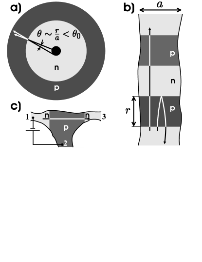
Figure 2: Ballistic MR devices with n-p junctions in graphene: (a) Corbino geometry; (b) series of n-p-n junctions, with the illustration of trajectories of electrons transmitted by the first junction for $B=0$ (left) and $B>B\ast$ (right); (c) three-terminal cavity.

A strongly selective quasiparticle transmission in Eqs. (1,20) can also be used for creating ballistic cavity-type structures in graphene, with non-local transport properties. In a three-terminal ’cavity’ shown in Fig. 2(c), a p-charging gate would produce two parallel n-p junctions, so that ballistic electrons emitted from the contact 1 and transmitted by the first junction would easily pass through the second and reach contact 3. As a result, a bias voltage applied between contacts 1 and 2 would generate current between contacts 1 and 3, thus giving rise to the trans-conductance $G_{12}^{13}$ with a strong magnetic field dependence,

$$G_{12}^{13}(B)\sim\frac{2e^{2}}{\pi h}\sqrt{\frac{a^{2}k_{F}}{d}}\;f(\tfrac{B}{B_{\ast}}).$$ (23)

The authors thank T. Ando, A. Geim, J. Jefferson, and E. McCann for useful discussions.  This project has been supported by the Lancaster-EPSRC Portfolio Partnership EP/C511743.

References

- (1) J.W. McClure, Phys. Rev. 104, 666 (1956); F.D.M. Haldane, Phys. Rev. Lett. 61, 2015 (1988); Y. Zheng and T. Ando, Phys. Rev. B 65, 245420 (2002); V.P. Gusynin and S.G. Sharapov, Phys. Rev. Lett. 95, 146801 (2005); A. Castro Neto, F. Guinea, and N. Peres, cond-mat/0509709; N. Peres, A. Castro Neto and F. Guinea, cond-mat/0512476
- (2) D. DiVincenzo, E. Mele, Phys. Rev. B 29, 1685 (1984)
- (3) G.W. Semenoff, Phys. Rev. Lett. 53, 2449 (1984)
- (4) R. Saito, G. Dresselhaus, M.S. Dresselhaus, Physical Properties of Carbon Nanotubes, Imperial College Press, London 1998
- (5) T. Ando, T. Nakanishi, and R. Saito, J. Phys. Soc. Japan 67, 2857 (1998); H. Suzuura and T. Ando, Phys. Rev. Lett. 89, 266603 (2002)
- (6) E. McCann and V.I. Fal’ko, Phys. Rev. Lett. 96, 086805 (2006)
- (7) K.S. Novoselov et al., Science 306, 666 (2004)
- (8) K.S. Novoselov et al., PNAS 102, 10451 (2005); J.S. Bunch et al., Nano. Lett. 5, 287 (2005); Y. Zhang et al., Phys. Rev. Lett. 94, 176803 (2005); C. Berger et al., J. Phys. Chem. B 108, 19912 (2004)
- (9) K.S. Novoselov et al., Nature 438, 197 (2005)
- (10) Y. Zhang et al., Nature 438, 201 (2005)
- (11) K. Novoselov et al, Nature Physics 2, 177 (2006)
- (12) Corners of the hexagonal Brilloin zone are , where and is the lattice constant. To use the same Dirac-type Hamiltonian in both valleys, we determine the two-component iso-spinor as in the valley () and in the valley (). In such notations, time reversal is described by , and spatial inversion (parity) by , where swaps valleys.
- (13) Everywhere below we shall use units .
- (14) Note that the transmitted quasiparticle on the other side of the junction have momentum .
- (15) L.I. Glazman et al, JETP Letters 48, 238 (1988)
- (16) This is close to the Fano factor for a graphene wire predicted in: J. Tworzydlo, B. Trauzettel, M. Titov, and C.W.J. Beenakker, cond-mat/0603315
- (17) P.A. Mello and N. Kumar, Quantum Transport in Mesoscopic Systems, Oxford University Press, 2004
- (18) M. Abramowitz and I. Stegun, Handbook of Mathematical Functions, Dover Publ. NY 1972, p.504
- (19) Energy averaging (thermal smearing) of the Fermi distribution and is equivalent to the averaging over a large ballistic phase accumulated bertween two np interfaces.