Distorted vortex lattice in a tetrahedral superconductor Distorted vortex lattice in a tetrahedral superconductor V. H. Dao, M. E. Zhitomirsky V. H. Dao, M. E. Zhitomirsky 13 January 2006*

Distorted vortex lattice in a tetrahedral superconductor

Abstract

Equilibrium shape and orientation of vortex lattice are studied for an $s$-wave tetrahedral superconductor in the vicinity of the upper critical field. The phase diagram, which includes transitions between rhombic and rectangular lattices, is constructed in the parameter space of the Ginzburg-Landau functional. The developed theory is applied to the heavy-fermion superconductor PrOs₄Sb₁₂. In a wide range of parameters the shape of the vortex lattice is only weakly dependent on temperature. The neutron scattering measurements of the vortex lattice in PrOs₄Sb₁₂ can be explained by a peculiarities of the tetrahedral symmetry group and are further supported by analysis of the appropriate band structure calculations.

74.20.De, 74.25.Qt

Hexagonal vortex lattice predicted for ideal isotropic superconductors [1, 2] is perturbed in real materials by crystalline anisotropy. Anisotropic nonlocal corrections within the Ginzburg-Landau theory or in the London approximation are determined by the Fermi surface geometry [3]. Their effect may result in a hexagonal-to-square vortex lattice transition observed in the past in the superconducting borocarbides [4, 5, 6, 7]. Anisotropy of the Cooper pairs wave function also gives rise to vortex lattice distortions. The line nodes of the $d_{x^{2}-y^{2}}$ superconducting gap in the high-$T_{c}$ cuprates favor, for example, a square vortex lattice [8, 9]. The flux line lattice (FLL) geometry provides, thus, a combined insight into the Fermi surface and the order parameter anisotropy.

Filled skutterudite compound PrOs₄Sb₁₂ has attracted significant attention in the past few years as a first example of Pr-based heavy fermion superconductor with $T_{c}=1.85$ K [10, 11, 12, 13, 14]. At present, controversy remains about the symmetry and the structure of the superconducting gap in PrOs₄Sb₁₂. The low-temperature scanning tunneling spectroscopy experiments by Suderow et al. [15] clearly demonstrate a finite superconducting gap over a large part of the Fermi surface. This finding is independently confirmed by an exponential low-temperature dependence of the nuclear relaxation rate $1/T_{1}$ [16], though absence of the coherence peak may point to anisotropic pairing. Recently, small angle neutron scattering measurements have found a distorted vortex lattice in PrOs₄Sb₁₂ at low fields and temperatures [17]. The observed distortion was attributed by Huxley et al. to an anisotropic multicomponent superconducting order parameter with point nodes. PrOs₄Sb₁₂ has, however, a rather unusual tetrahedral $T_{h}$ point group. This group contains three-fold rotations about cube diagonals but no four-fold rotations in contrast to the other cubic groups $O$ and $O_{h}$. Investigation of the shape of FLL has not been done to our knowledge for such superconductors. In the present work we investigate the geometry of FLL in tetrahedral superconductors within the nonlocal Ginzburg-Landau theory for a conventional $s$-wave order parameter.

The Ginzburg-Landau (GL) energy density functional for an $s$-wave superconducting order parameter $\Psi$ derived from the BCS theory has the standard form:

$$F_{GL}=\Psi^{*}({\bf x})\left(\alpha+{\cal F}_{\Pi}\right)\Psi({\bf x})+\frac{\beta}{2}|\Psi({\bf x})|^{4}+\frac{h^{2}}{8\pi}\ .$$ (1)

Here $\alpha=(1-T/T_{c})$, $T_{c}$ is the transition temperature, and $\beta=7\zeta(3)/(4\pi T_{c})^{2}$. The gradient terms

$${\cal F}_{\Pi}=\sum_{n=1}^{\infty}\sum_{i_{1}\ldots i_{2n}}K_{i_{1}\dots i_{2n}}\;\;\Pi_{i_{1}}\ldots\Pi_{i_{2n}}$$ (2)

are expanded into even powers of the operator $\Pi_{i}=-i\partial_{i}+(2\pi/\Phi_{0})A_{i}$, $\Phi_{0}$ being the flux quantum. Expansion coefficients are expressed via the Fermi surface averages of the components of the Fermi velocity ${\bf v}_{F}$ as

$$K_{i\ldots j}=\frac{(-1)^{n+1}}{(2\pi T_{c})^{2n}}(2-\frac{1}{2^{2n}})\zeta(2n+1)\langle v_{Fi}\dots v_{Fj}\rangle_{\rm FS}.$$ (3)

The tetrahedral point symmetry $T_{h}$ imposes certain relations between the gradient term coefficients:

$$K_{x^{2}}=K_{y^{2}}=K_{z^{2}},\ \ \ \ \ \ \ \ \ \ \ K_{x^{4}}=K_{y^{4}}=K_{z^{4}},$$

$$K_{x^{2}y^{2}}=K_{x^{2}y^{2}}=K_{y^{2}z^{2}},\ \ \ K_{x^{6}}=K_{y^{6}}=K_{z^{6}},$$ (4)

$$K_{x^{4}y^{2}}=K_{y^{4}z^{2}}=K_{z^{4}x^{2}},\ \ \ K_{x^{2}y^{4}}=K_{y^{2}z^{4}}=K_{z^{2}x^{4}}.$$

Note, that for the tetrahedral group $K_{x^{4}y^{2}}\neq K_{x^{2}y^{4}}$.

Let us now assume that an external magnetic field is applied along the $\hat{z}$-axis. Considering only solutions, which are uniform along the field direction ($\Pi_{z}\Psi\equiv 0$), the gradient terms are simplified to

$${\cal F}_{2} = K_{x^{2}}\left(\Pi_{x}^{2}+\Pi_{y}^{2}\right)\ ,$$

$${\cal F}_{4} = K_{x^{4}}\left(\Pi_{x}^{4}+\Pi_{y}^{4}\right)+K_{x^{2}y^{2}}\{\Pi_{x}^{2}\Pi_{y}^{2}\}\ ,$$ (5)

$${\cal F}_{6} = K_{x^{6}}\left(\Pi_{x}^{6}+\Pi_{y}^{6}\right)+K_{x^{4}y^{2}}\{\Pi_{x}^{4}\Pi_{y}^{2}\}+K_{x^{2}y^{4}}\{\Pi_{x}^{2}\Pi_{y}^{4}\}.$$

In the above expressions $\{\cdots\}$ denotes a sum over all possible permutations of the gradient operators $\Pi_{i}$ and $\Pi_{j}$.

The upper critical field $H_{c2}$ is determined by the linearized GL equation, which can be conveniently written in terms of the Landau level operators $\hat{a}$ and $\hat{a}^{\dagger}$: $\hat{a}=\sqrt{\Phi_{0}/4\pi H}(\Pi_{x}-i\Pi_{y})$. Rotation by angle $\varphi$ about $\hat{z}$-axis transforms the Landau level operators into $e^{-i\varphi}\hat{a}$ and $e^{i\varphi}\hat{a}^{\dagger}$. After some algebra, the gradient terms (5) are expressed as

$${\cal F}_{2} = h(2\hat{n}+1)\ ,$$

$${\cal F}_{4} = h^{2}\left[k_{40}(2\hat{n}^{2}+2\hat{n}+1)+k_{44}(\hat{a}^{4}+\hat{a}^{\dagger 4})\right],$$

$${\cal F}_{6} = h^{3}\left[k_{60}\hat{n}_{60}+k_{62}(\hat{n}_{62}\hat{a}^{2}+\hat{a}^{\dagger 2}\hat{n}_{62})\right.$$ (6)

$$\left.+k_{64}(\hat{n}_{64}\hat{a}^{4}+\hat{a}^{\dagger 4}\hat{n}_{64})+k_{66}(\hat{a}^{6}+\hat{a}^{\dagger 6})\right],$$

where $h=2\pi HK_{x^{2}}/\Phi_{0}$ is a dimensionless magnetic field and

$$k_{40} = 3(K_{x^{4}}+K_{x^{2}y^{2}})/2K_{x^{2}}^{2}\ ,$$

$$k_{44} = (K_{x^{4}}-3K_{x^{2}y^{2}})/2K_{x^{2}}^{2}\ ,$$

$$k_{60} = (2K_{x^{6}}+3K_{x^{4}y^{2}}+3K_{x^{2}y^{4}})/8K_{x^{2}}^{3}\ ,$$ (7)

$$k_{62} = (K_{x^{4}y^{2}}-K_{x^{2}y^{4}})/8K_{x^{2}}^{3}\ ,\ \ k_{66}=-15k_{62}\ ,$$

$$k_{64} = (2K_{x^{6}}-5K_{x^{4}y^{2}}-5K_{x^{2}y^{4}})/8K_{x^{2}}^{3}\ .$$

The level-number operator $\hat{n}=\hat{a}^{\dagger}\hat{a}$ and its polynomials $\hat{n}_{60}=(20\hat{n}^{3}+30\hat{n}^{2}+40\hat{n}+15)$, $\hat{n}_{62}=(15\hat{n}^{2}+63\hat{n}+45)$, $\hat{n}_{64}=(6\hat{n}+15)$ are invariant with respect to an arbitrary rotation about the $\hat{z}$-axis. The discrete rotations of the point crystal group are responsible for the appearance of $\hat{a}^{n}$ terms. In particular, the operators $\hat{a}^{2}$ and $\hat{a}^{6}$ break the four-fold rotational symmetry about $\hat{z}$ and discriminate between the $\hat{x}$- and the $\hat{y}$-axes.

We use the standard procedure to determine the FLL geometry in the vicinity of the upper critical field [1, 2]. Previously, such an approach has been applied for superconductors with tetragonal [6, 7, 18, 19], orthorhombic [20], and hexagonal [21] crystal structures. Solution of the linearized GL equations obtained from Eqs. (1) and (6) is expanded in the Landau levels up to the sixth order:

$$\Psi=\lambda\psi\ ,\ \psi=f_{0}+c_{2}e^{2i\varphi}f_{2}+c_{4}e^{4i\varphi}f_{4}+c_{6}e^{6i\varphi}f_{6}\ ,$$ (8)

where $f_{n}=(\hat{a}^{\dagger})^{n}f_{0}/\sqrt{n!}$ and $\hat{a}f_{0}=0$. In order to construct a periodic vortex structure at the zeroth Landau level $f_{0}$ it is convenient to go from a laboratory frame determined by the crystal axes to a rotated frame such that a new $\hat{x}$-axis points between a pair of nearest-neighbor vortices and is rotated by angle $\varphi$ with respect to the crystal axis. The vector potential is chosen in the Landau gauge ${\bf A}=(-Hy,0,0)$ and the periodic solution with one flux quantum per unit cell is written as

$$f_{0}({\bf r})=\sum_{m}\exp\Bigl{[}-\pi i\rho m^{2}+\frac{2\pi}{a}imx-\frac{\pi H}{\Phi_{0}}(y-ma\sigma)^{2}\Bigr{]}.$$ (9)

The basis vectors of the FLL are $(a,0,0)$ and $(a\rho,a\sigma,0)$ in the rotated frame, which satisfy the one-flux-quantum condition $Ha^{2}\sigma=\Phi_{0}$.

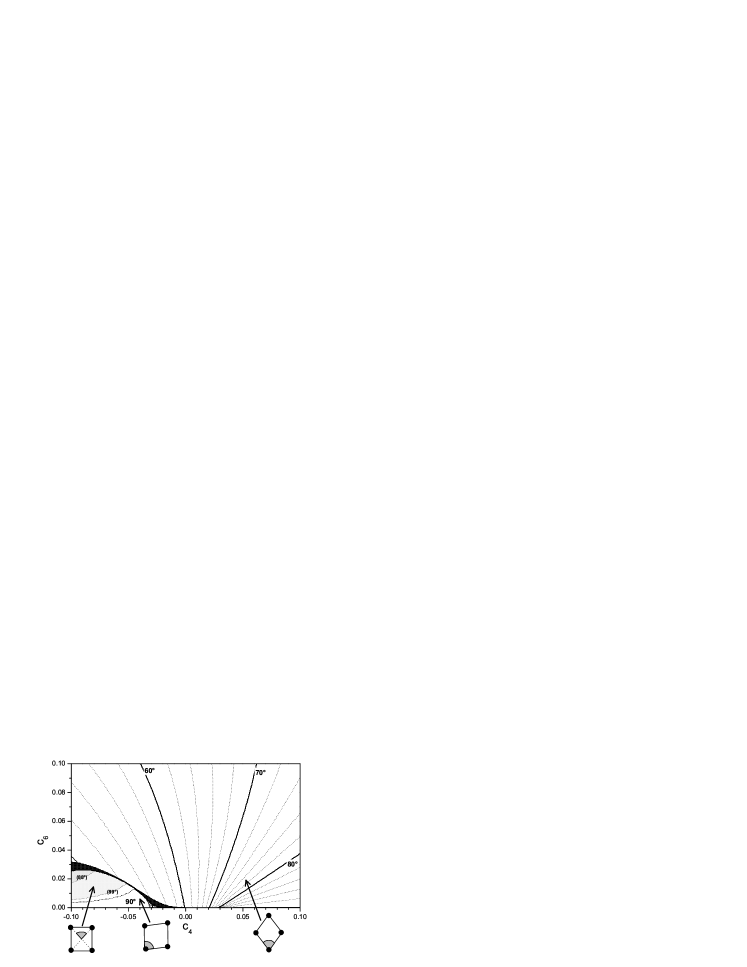
Figure 1: Fig.1: Geometry of the FLL unit cell as a function of $c_{4}$ and $c_{6}$. Lines indicate corresponding values of angles, which parameterize a rhombic or a rectangular unit cells

The expansion coefficients in Eq. (8) are found for the eigensolution of the linearized GL equation as a perturbation expansion in a small parameter $\alpha$:

$$c_{4}=\frac{\sqrt{6}}{4}k_{44}\alpha\ ,\ c_{2}=-\frac{45}{2\sqrt{2}}k_{62}\alpha^{2}\ ,\ c_{6}=-\sqrt{5}k_{66}\alpha^{2}\ ,$$ (10)

whereas the upper critical field is given by

$$h_{c2}=-\alpha-k_{40}\alpha^{2}+(15k_{60}-2k_{40}^{2}-3k_{44}^{2})\alpha^{3}\ .$$ (11)

Neglecting the magnetic field contribution to the free energy $h^{2}/8\pi$ in the large-$\kappa$ limit we obtain for the energy density

$$\langle F_{GL}\rangle=\lambda^{2}\langle\psi^{*}(\alpha+{\cal F}_{\Pi})\psi\rangle+\lambda^{4}\frac{\beta}{2}\langle|\psi|^{4}\rangle\ ,$$ (12)

where $\langle f\rangle=(1/V)\int dr^{3}f({\bf r})$. The quadratic term in the above equation is calculated as $\langle|f_{0}|^{2}\rangle(h-h_{c2})(1-2k_{40}\alpha)$. Then, straightforward minimization of the energy density (12) with respect to $\lambda$ yields

$$\langle F_{GL}\rangle=-\frac{(h-h_{c2})^{2}(1-2k_{40}\alpha)^{2}}{2\beta\langle|\psi|^{4}\rangle/\langle|f_{0}|^{2}\rangle^{2}}\ .$$ (13)

The equilibrium distribution of the order parameter $\Psi({\bf r})$ is found by minimizing the geometrical factor

$$\beta_{A}=\langle|\psi|^{4}\rangle/\langle|f_{0}|^{2}\rangle^{2}\ .$$ (14)

This generalized Abrikosov’s parameter is a function of only three variables $\rho$, $\sigma$, and $\varphi$. An explicit calculation yields

$$\beta_{A}=\sqrt{\sigma}\sum_{m,n}\exp{\left[2\pi i\rho(m^{2}\!-n^{2})-2\pi\sigma(m^{2}\!+n^{2})\right]}\,I_{m,n},$$ (15)

where summation goes over all integer and half-integer pairs $(m,n)$. Function $I_{m,n}$ is defined by an integral

$$I_{m,n} = \sqrt{\frac{2}{\pi}}\int dye^{-2y^{2}}P\bigl{(}y+\sqrt{2\pi\sigma}m\bigr{)}\,P\bigl{(}y-\sqrt{2\pi\sigma}m\bigr{)}$$ (16)

$$\mbox{}\times P^{*}(y+\sqrt{2\pi\sigma}n)P^{*}(y-\sqrt{2\pi\sigma}n)\ ,$$

where

$$P(y)=1+c_{2}e^{2i\varphi}H_{2}(y)+c_{4}e^{4i\varphi}H_{4}(y)+c_{6}e^{6i\varphi}H_{6}(y)$$ (17)

and $H_{n}(y)$ are the Hermite’s polynomials. If we keep, for simplicity, only the terms, which are linear in $c_{n}$, then the Abrikosov parameter is reduced to

$$\beta_{A}\approx\beta_{0}+4{\Real}(c_{2}e^{2i\varphi}\beta_{2}+c_{4}e^{4i\varphi}\beta_{4}+c_{6}e^{6i\varphi}\beta_{6})\ ,$$ (18)

where

$$\beta_{k}=\langle f_{0}^{*2}f_{0}f_{k}\rangle/\langle|f_{0}|^{2}\rangle^{2}\ .$$ (19)

Function $\beta_{0}(\rho,\sigma)$ is the standard energy parameter for an isotropic superconductor [1], which is given by Eq. (15) with $I^{(0)}_{m,n}=1$ [2]. The other functions $\beta_{k}$ are obtained from Eq. (15) by substituting the corresponding $I^{(k)}_{m,n}$:

$$I^{(2)}_{m,n} = \frac{1}{\sqrt{2}}\Bigl{(}4\pi\sigma n^{2}-\frac{1}{2}\Bigr{)}\ ,$$

$$I^{(4)}_{m,n} = \frac{1}{\sqrt{6}}\Bigl{(}8\pi^{2}\sigma^{2}n^{4}-6\pi\sigma n^{2}+\frac{3}{8}\Bigr{)}\ ,$$ (20)

$$I^{(6)}_{m,n} = \frac{1}{3\sqrt{5}}\Bigl{(}16\pi^{3}\sigma^{3}n^{6}-30\pi^{2}\sigma^{2}n^{4}+\frac{45}{4}\pi\sigma n^{2}-\frac{15}{32}\Bigr{)}.$$

Hexagonal vortex lattice with $\rho=1/2$ and $\sigma=\sqrt{3}/2$ corresponds to the absolute minima of functions $\beta_{0}(\rho,\sigma)$ and $\beta_{6}(\rho,\sigma)$. The other two functions $\beta_{4}$ and $\beta_{2}$ tend to stabilize a square and a distorted triangular lattices, respectively. Their competition yields a rich phase diagram of a tetrahedral superconductor. In finding the lowest energy vortex lattice we have kept also additional terms in $\beta_{A}$, which are proportional to high-orders of $c_{n}$.

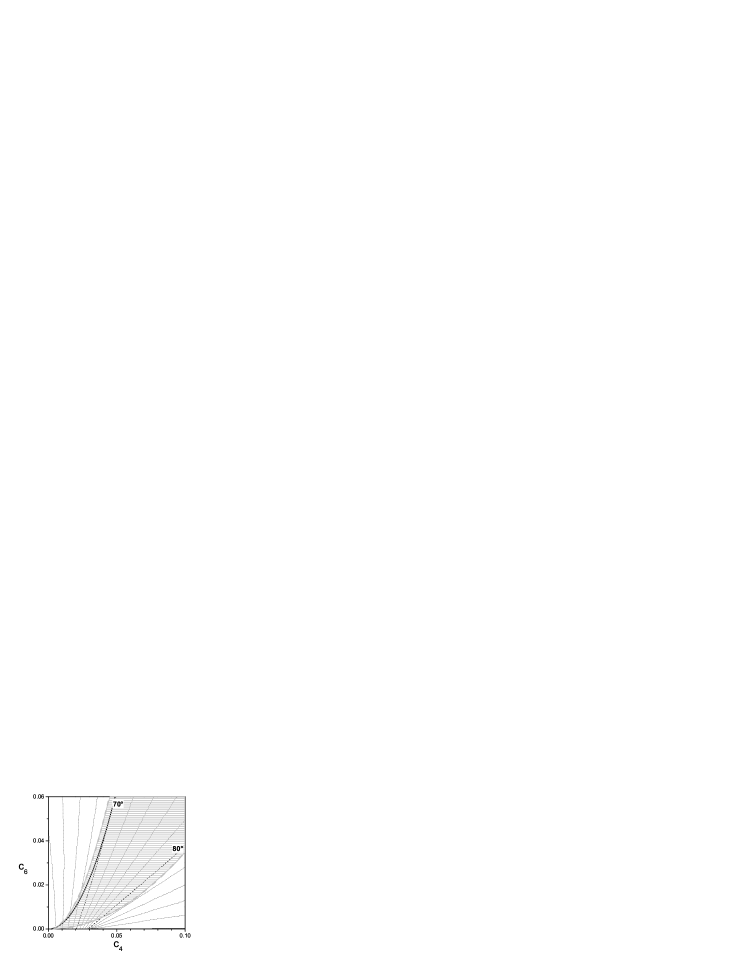
Figure 2: Fig.2: Expansion of the right part of fig.1. The shaded region is composed by parabolas $c_{6}(T)\propto c_{4}(T)^{2}$; the black line is defined by $c_{6}=25c_{4}^{2}$

Equilibrium form and orientation of the vortex lattice in a tetrahedral superconductor should be obtained by minimizing $\beta_{A}(\rho,\sigma,\varphi)$ for different sets of the parameters $\alpha$ and $k_{ij}$ in the GL functional. The task is considerably simplified if the expansion of $\psi$ in Eq. (8) is rapidly converging, e.g., near $T_{c}$ or for a superconductor with a weak anisotropy. In such a case, a set of the effective parameters can be reduced to $c_{4}$, which is determined by the lowest order anisotropy in quartic terms, and $c_{6}$, which quantifies the $x$–$y$ discrimination introduced by the tetrahedral symmetry. Since $c_{2}\propto c_{6}$ in the leading order in $\alpha$, we fix $c_{2}=-3/(2\sqrt{10})c_{6}\approx-0.47c_{6}$. The energy parameter $\beta_{A}$ is, then, numerically minimized with the conjugate gradient method. The parameter space is further restricted to $c_{6}\geq 0$ since a change of the sign of $c_{6}$ corresponds to a rotation of the coordinate frame by $\varphi=90^{\circ}$.

Our main results are presented in fig.1, where the geometry adopted by the FLL is plotted for different values of $c_{4}$ and $c_{6}$. The considered region in the parameter space is divided into two parts corresponding to highly symmetric vortex lattices separated by a transition region colored in black. In the main area, the whole $(c_{4},c_{6})$ plane apart from the lower left corner, the unit cell has a rhombic shape with the longest diagonal parallel to the $\hat{y}$-axis. The apex angle of a rhombus $\theta$ varies from 50^∘ to 90^∘ as indicated by thin dotted lines.

Since $c_{4}={\cal O}(\alpha)$ and $c_{6}={\cal O}(\alpha^{2})$, an evolution along the $H_{c2}(T)$-curve follows approximately a parabolic path in the $(c_{4},c_{6})$-phase diagram, which starts at the origin $c_{4}=0$ and $c_{6}=0$. For a certain range of parameters, the apex angle $\theta$ along such an $H_{c2}(T)$-path does not change significantly with temperature. For example, $\theta$ remains between $70^{\circ}$ and $80^{\circ}$ in the shaded area of fig.2 composed by a set of parabolas given by $c_{6}/c_{4}^{2}=-16\sqrt{5}k_{66}/6k_{44}^{2}$ with

$$-5\leq k_{66}/k_{44}^{2}\leq-0.6\ .$$ (21)

The reason for such a weak dependence is a cancellation of two opposite tendencies determined by $\beta_{2}(\rho,\sigma)$ and $\beta_{4}(\rho,\sigma)$, see Eq. (19). If the crystal would have the cubic or the tetragonal symmetry, $c_{6}$ is zero and the apex angle increases almost linearly between $60^{\circ}$ and $90^{\circ}$, with a phase transition into a square lattice afterwards. The present investigation shows that the tetrahedral symmetry introduces a fundamental difference via a sixth-order gradient terms.

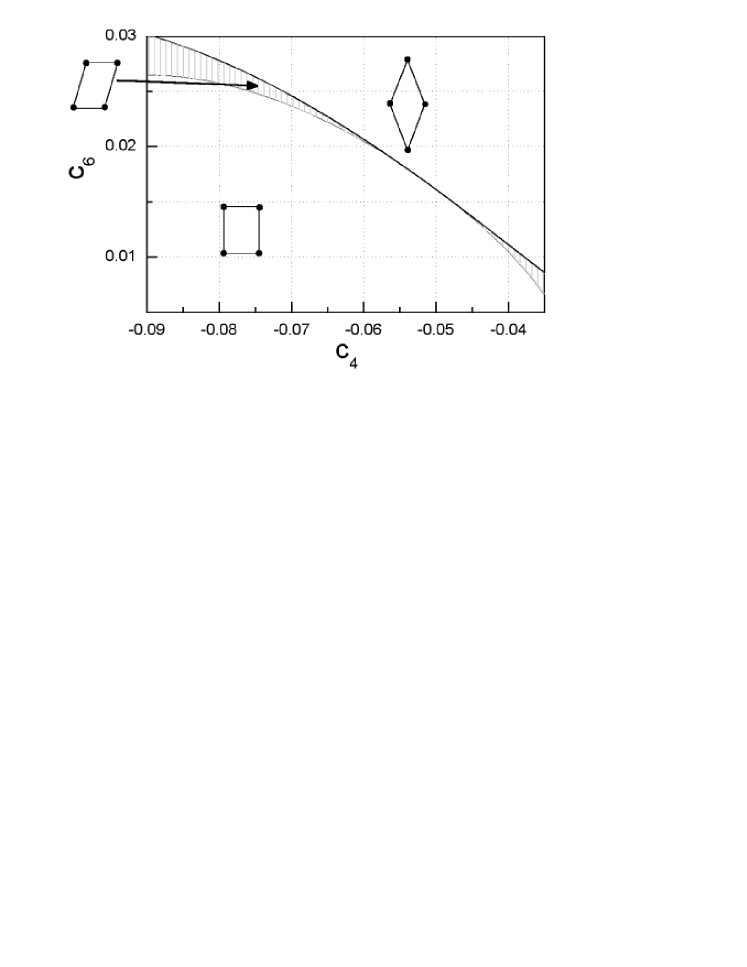
Figure 3: Fig.3: Expansion of the left side of fig.1: transition region between the vortex unit cells of rhombic and rectangular shapes

In the lower left corner of the phase diagram, for $c_{4}<0$ and small $c_{6}$, the shape of the vortex unit cell changes via a second-order transition from a rhombus with the longest diagonal oriented by $45^{\circ}$ from the $\hat{x}$-axis to a rectangle with the longest side along the $\hat{y}$-axis. When $c_{4}$ decreases, the small apex angle of the rhombus goes from 60^∘ to 90^∘. The two regions on the phase diagram are separated by a transition region (shown in black), where the unit cell of FLL has no mirror symmetry. Fig.3 illustrates that a transformation of the unit cell corresponds to a shear instability of the vortex lattice: vortex chains in the rectangular lattice slide along one of the directions such that the lattice turns into a centered rectangular (rhombic) lattice with the same volume of the unit cell and the same side ratio. This transformation goes via two second-order transitions for $c_{4}<-0.06$, whereas for $-0.055<c_{4}<-0.048$ the transition is of the first order. As a last remark, we would like to point at a peculiar possibility for a tetrahedral superconductor with negative $c_{4}$. While moving along the $H_{c2}(T)$ line towards low temperatures, the vortex lattice first changes from a triangular one into a rectangular lattice and then transforms back into a distorted triangular lattice.

Finally, we shall apply the above results to PrOs₄Sb₁₂. Topology of the Fermi surface of this material has been studied by the de Haas-van Alphen measurements and compared to the results of the LDA+$U$ band structure calculations by Sugawara et al. [22, 23]. The Fermi surface is composed of three sheets: one of the 48th band and two of the 49th band. The contribution to the density of states from the 48th band is relatively small: $N_{48}(0)\sim 0.04N_{49}(0)$. Besides, only a small Fermi velocity in the 49th band is capable to account for a large value of the upper critical field at zero temperature $H_{c2}(0)=2.2$ T [10]. Accordingly, we assume that the active band, which is responsible for superconductivity in PrOs₄Sb₁₂, is the 49th band, whereas the 48th band plays a passive role and may have a smaller gap amplitude as suggested by Seyfarth et al. [14].

Table 1: Table I: Fermi surface averages of different combinations of the components of the Fermi velocity $\langle v_{Fx}^{k}v_{Fy}^{l}v_{Fz}^{m}\rangle_{\rm FS}$ for the 49th band in units of ($10^{5}$ m/s)^k+l+m.

$klm$			$\alpha$-sheet		$\gamma$-sheet		combined
200			$2.19$		$1.46$		$1.61$
400			$14.7$		$6.36$		$8.11$
220			$1.51$		$1.63$		$1.60$
600			$127.$		$45.0$		$62.2$
420			$5.69$		$3.74$		$4.15$
240			$4.49$		$8.75$		$7.85$
222			$1.03$		$0.63$		$0.714$

The band structure data for 195 $\bf k$-points in the irreducible part of the Brillouin zone of PrOs₄Sb₁₂ have been previously used in the comparison between LDA results and de Haas-van Alphen data [22]. We interpolated between these data points using appropriate lattice harmonics and, then, calculated numerically the Fermi surface averages for the 49th band using a much smaller mesh in the momentum space. The combined averages have been obtained by a sum of the two contributions weighted according to partial densities of states $N^{\alpha}_{49}/N^{\gamma}_{49}\approx 0.27$. The results are summarized in Table I. Using Eqs. (3) and (7) we find for the dimensionless gradient constants $k_{44}=-0.29$, $k_{66}=-0.35$ such that $k_{66}/k_{44}^{2}=-4.3$ and

$$c_{6}(T)/c_{4}(T)^{2}\approx 25.0\ .$$ (22)

The above relation is illustrated in fig.2 by a solid line. For $c_{4}(T)\geq 0.02$, which corresponds to $|\alpha|\geq 0.12$ and $T<0.9T_{c}$, the vortex lattice has a rhombic unit cell with a nearly $T$-independent apex angle $\theta=70^{\circ}$. For a rhombic lattice this angle coincides exactly with the angle between two reciprocal lattice vectors. The latter angle has been measured in the neutron scattering experiment [17] and is equal to $\theta\approx 75\pm 5^{\circ}$. Thus, there is a good agreement between our calculation and the experimental data on PrOs₄Sb₁₂. We emphasize again, that in a tetrahedral superconductor such a stable distortion of a hexagonal vortex lattice arises due to a competition between several anisotropic gradient terms. When comparing the above results with experimental data one should, of course, bear in mind that applicability regions are somewhat different. Formally, our calculation has been restricted to the vicinity of $H_{c2}$, but is valid in a wider range of applied fields $H>0.2H_{c2}$ in high-$\kappa$ materials such as PrOs₄Sb₁₂ ($\kappa\approx 29$). The temperature range is in the GL regime $0.6T_{c}<T<0.9T_{c}$, whereas the neutron measurements have been performed for $T<0.45T_{c}$. Further investigations of the shape of the vortex lattice in tetrahedral superconductors in the London limit at low temperatures would be, therefore, useful.

A different confirmation of our analysis can be provided by angle dependence of the upper critical field since the amplitude of the modulations are related to the anisotropy of the Fermi surface [3, 24, 25]. For example, a perturbation calculation yields the main contribution to the [001]-plane four-fold modulation:

$$\frac{H_{c2}(\phi)}{H_{c2}(0)}=1+\frac{3}{8}\,\alpha k_{44}\bigl{(}\cos{4\phi}-1\bigr{)}\ ,$$ (23)

where $\phi$ is angle between an applied magnetic field and the $\hat{x}$-axis.

We are indebted to V. P. Mineev for stimulating discussion and to H. Harima for providing us the band structure data for PrOs₄Sb₁₂.

References

- [1] A. A. Abrikosov, Zh. Éksp. Teor. Fiz. 32, 1442 (1957) [Sov. Phys. JETP 5, 1174 (1957)].
- [2] D. Saint-James, E. J. Thomas, and G. Sarma, Type II Superconductivity (Pergamon Press, Oxford, 1969).
- [3] K. Takanaka, Prog. Theor. Phys. 46, 1301 (1971); K. Takanaka, in Anisotropy Effects in Superconductors, edited by H. Weber (Plenum, New York, 1977).
- [4] U. Yaron, P. L. Gammel, A. P. Ramirez, D. A. Huse, D. J. Bishop, A. I. Goldman, C. Stassis, P. C. Canfield, K. Mortensen, and M. R. Eskildsen, Nature (London) 382, 236 (1996).
- [5] Y. De Wilde, M. Iavarone, U. Welp, V. Metlushko, A. E. Koshelev, I. Aranson, and G. W. Crabtree, Phys. Rev. Lett. 78, 4273 (1997).
- [6] K. Park and D. A. Huse, Phys. Rev. B 58, 9527 (1998).
- [7] A. D. Klironomos and A. T. Dorsey, Phys. Rev. Lett. 91, 097002 (2003).
- [8] H. Won and K. Maki, Europhys. Lett. 30, 421 (1995).
- [9] I. Affleck, M. Franz, and M. Amin, Phys. Rev. B 55, R705 (1997).
- [10] E. D. Bauer, N. A. Frederick, P. C. Ho, V. S. Zapf, and M. B. Maple, Phys. Rev. B 65, 100506 (2002).
- [11] M. B. Maple, P.-C. Ho, V. S. Zapf, N. A. Frederick, E. D. Bauer, W. M. Yuhasz, F. M. Woodward and J. W. Lynn, J. Phys. Soc. Jpn. 71, 23 (2002).
- [12] R. Vollmer, A. Faißt, C. Pfleiderer, H. v. L hneysen, E. D. Bauer, P.-C. Ho, V. Zapf, and M. B. Maple, Phys. Rev. Lett. 90, 057001 (2003).
- [13] M.-A. Méasson, D. Braithwaite, J. Flouquet, G. Seyfarth, J. P. Brison, E. Lhotel, C. Paulsen, H. Sugawara, and H. Sato, Phys. Rev. B 70, 064516 (2004).
- [14] G. Seyfarth, J. P. Brison, M.-A. Méasson, J. Flouquet, K. Izawa, Y. Matsuda, H. Sugawara, and H. Sato, Phys. Rev. Lett. 95, 107004 (2005).
- [15] H. Suderow, S. Viera, J. D. Strand, S. Bud’ko, and P. C. Canfield, Phys. Rev. B 69, 060504 (2004).
- [16] H. Kotegawa, M. Yogi, Y. Imamura, Y. Kawasaki, G.-q. Zheng, Y. Kitaoka, S. Ohsaki, H. Sugawara, Y. Aoki, and H. Sato, Phys. Rev. Lett. 90, 027001 (2003).
- [17] A. D. Huxley, M.-A. Measson, K. Izawa, C. D. Dewhurst, R. Cubitt, B. Grenier, H. Sugawara, J. Flouquet, Y. Matsuda, and H. Sato, Phys. Rev. Lett. 93, 187005 (2004).
- [18] D. Chang, C.-Y. Mou, B. Rosenstein, and C. L. Wu, Phys. Rev. B 57, 7955 (1998).
- [19] D. F. Agterberg, Phys. Rev. B 58, 14484 (1998).
- [20] Q. Han and L. Zhang, Phys. Rev. B 59, 11579 (1999).
- [21] M. E. Zhitomirsky and V. H. Dao, Phys. Rev. B 69, 054508 (2004).
- [22] H. Sugawara, S. Osaki, S. R. Saha, Y. Aoki, H. Sato, Y. Inada, H. Shishido, R. Settai, Y. Onuki, H. Harima, and K. Oikawa, Phys. Rev. B 66, 220504 (2002).
- [23] H. Harima and K. Takegahara, Physica B 359-361, 920 (2005).
- [24] H. Teichler, Phys. Stat. Sol. (b) 69, 501 (1975).
- [25] V. H. Dao and M. E. Zhitomirsky, Eur. Phys. J. B 44, 183 (2005).