Random and Correlated Roughening in Slow Fracture by Damage Nucleation

Abstract

We address the role of the nature of material disorder in determining the roughness of cracks which grow by damage nucleation and coalescence ahead of the crack tip. We highlight the role of quenched and annealed disorders in relation to the length scales $d$ and $\xi_{c}$ associated with the disorder and the damage nucleation respectively. In two related models, one with quenched disorder in which $d\simeq\xi_{c}$, the other with annealed disorder in which $d\ll\xi_{c}$, we find qualitatively different roughening properties for the resulting cracks in 2-dimensions. The first model results in random cracks with an asymptotic roughening exponent $\zeta\approx 0.5$. The second model shows correlated roughening with $\zeta\approx 0.66$. The reasons for the qualitative difference are rationalized and explained.

I Introduction

When cracks develop slowly via the nucleation of damage ahead of the tip, the crack surfaces left behind appear to be rough. A question of great interest is what is the scaling exponent that characterizes the roughening of such surfaces and how to relate the value of the exponent to the physical phenomena that govern the crack propagation. For cracks surfaces in 2+1 dimensions the anisotropy of the fracture experiment results in a number of scaling exponents, making the attainment of a satisfactory theory quite difficult 05BPS . On the other hand, for cracks in quasi 2-dimensional samples, where the resulting surfaces are 1+1 dimensional graphs (rupture lines), the issues are clear at least in the sense that there exists one well-defined scaling exponent. This is conveniently defined by measuring $y(x)$ where $y$ is the height of the graph above the Euclidean coordinate $x$ that defines the crack direction and then defining some measure of the height fluctuations, for example

$$h(r)\equiv\left<Max\left\{y(\tilde{x})\right\}_{x<\tilde{x}<x+r}-Min\left\{y(\tilde{x})\right\}_{x<\tilde{x}<x+r}\right>_{x}\ .$$ (1)

For self-affine graphs the scaling exponent $\zeta$ is defined via the scaling relation

$$h(r)\sim r^{\zeta}\ .$$ (2)

It is well known that random graphs are consistent with $\zeta=0.5$, whereas positively (negatively) correlated graphs are characterized by $\zeta>0.5$ ($\zeta<0.5)$. Experiments on 2-dimensional samples tend to report scaling exponents in the range $\zeta\approx 0.65\pm 0.04$ 93KHW ; 94EMHR ; 03SAN , indicating the existence of positive correlations between successive crack segments.

In recent work a model was proposed in 1+1 dimensions for such slow crack propagation via damage nucleation and coalescence ahead of the crack tip 04BMPa ; 05ABKMP . A crucial aspect of this model is the existence of a typical length scale $\xi_{c}$ ahead of the crack tip where damage nucleation can take place 99BP . A physical picture that might support such a scenario (though definitely not a unique one) is that a small plastic zone of linear dimension $\xi_{c}$ forms around the crack tip and the relevant damage units involved in the process are plastic voids. The idea is that since plastic deformation is typically associated with a limiting stress level (denoted the “yield stress”) $\sigma_{{}_{\rm Y}}$, the purely linear elastic divergent stresses are cut off such that they cannot reach a critical level required for the nucleation of voids at the crack tip. It is claimed that such critical levels of stress can be attained approximately near the outer boundary of the plastic zone, i.e. the elastic-plastic boundary. Whenever a void is nucleated in this region, it evolves and eventually coalesces with the current crack tip to form a new crack configuration. The crack then evolves by successive applications of such nucleation and coalescence events. Refs. 04BMPa ; 05ABKMP demonstrated that the rupture lines generated by this model are self-affine rough graphs with a correlated scaling exponent $\zeta\approx 0.66$. Not only the value of the roughness exponent is found to be significantly above the random walk exponent $\zeta=0.5$, it also appears close to the measured one 93KHW ; 94EMHR ; 03SAN . The aim of this paper is to gain a deeper understanding of the origin of this result.

An essential question asked in the context of any such fracture growth model is how to represent and incorporate the effect of material disorder. This issue is important since it asks how small scale features affect large scale properties, for example the power-law scaling of Eq. (2) that indicates a lack of characteristic length scale. To our knowledge there had been no systematic study of the role of the nature of material disorder in determining the roughness of cracks in 1+1 dimensions. Our aim here is to shed some light on this issue by demonstrating that different views of material disorder and the associated length scales have a qualitative effect on the scaling properties of rupture lines. To this aim we elaborate on the type of material disorder adopted in the model described briefly above - referred to below as model A - and present a new model - referred to below as model B - that incorporates a different picture of material disorder. In model B the disorder is quenched, and the stochasticity associated with the material heterogeneities is fixed a-priori in space and time. In model A the disorder is “annealed” in the sense that the stochasticity depends on the actual state of the system. Whenever the disorder has some spatial characteristic scale we denote it by $d$ and call it the “disorder length” that should be compared to the previously introduced length $\xi_{c}$. Thus model A is characterized by annealed disorder and $d\ll\xi_{c}$, while model B is characterized by quenched disorder and $d\simeq\xi_{c}$. One of the points of this paper is that this change in material disorder in model B is sufficient to destroy the positive correlations between successive crack segments observed in model A, changing the universality class of the model and ending up with a random graph with an asymptotic scaling exponent $\zeta\approx 0.5$.

In Sect. II we present in more detail model A and recall its results, elaborating on the way in which material disorder is incorporated into the model. We then explain the modifications leading to model B. In Sect. III we present the new results for model B, compare them with model A and clarify the origin of the qualitative differences between them. Sect. IV offers a summary and some concluding remarks.

II Crack propagation by damage nucleation and coalescence

II.1 A non-perturbative calculation of the linear-elastic stress fields

The mathematical difficulty in developing a theory for the morphology of fracture surfaces is the necessity of calculating the linear-elastic stress fields for highly non-regular crack paths. Typically, the stress conditions near the crack tip depend non-linearly on the crack path $y(x)$. Formally, one has to solve the bi-Laplace equation for the Airy stress potential $\chi(x,y)$ 86LL

$$\Delta\Delta\chi(x,y)=0\ ,$$ (3)

in the infinite plane with traction-free boundary conditions on the crack surfaces

$$\sigma_{xn}(s)=\sigma_{yn}(s)=0\ .$$ (4)

Here $s$ is the arc-length parametrization of the crack shape and the $\sigma_{in}(s)$ denotes the stress acting in the $i$-th direction on a segment whose out-ward normal is the normal to the crack face at $s$. The stress tensor field $\sigma_{ij}$ is derivable form the Airy stress potential $\chi(x,y)$ according to

$$\sigma_{xx}=\frac{\partial^{2}\chi}{\partial y^{2}}\!\ ;\quad\sigma_{xy}=-\frac{\partial^{2}\chi}{\partial x\partial y}\!\ ;\quad\sigma_{yy}=\frac{\partial^{2}\chi}{\partial x^{2}}\ .$$ (5)

The relevant experimental configuration for our purpose is that of global mode I fracture in which a system containing initially a straight crack in the $x$ direction, subjected to a stress applied in the direction $y$, perpendicular to the crack. At infinity we write the boundary conditions

$$\sigma_{xx}(\infty)=0\!\ ;\quad\sigma_{yy}(\infty)=\sigma^{\infty}\!\ ;\quad\sigma_{xy}(\infty)=0\ ,$$ (6)

where $\sigma^{\infty}$ is assumed to be constant.

Note that even though the initial configuration is that of a straight crack, with material disorder the crack might deviate from the straight path, attaining an arbitrary rough shape. Solving the bi-Laplace equation with boundary conditions on such an arbitrary boundary is quite a formidable task. Recently, we have developed a general method of solution based on iterated conformal maps 04BMPb . In this method, one starts with a crack for which the conformal map from the exterior of the unit circle to the exterior of the crack is known. For example, in our case we start with a long straight crack in the form of a mathematical branch-cut, representing the common experimental practice of introducing the sample with a notch in order to localize the fracture process in a controlled way. We can then grow the crack by little steps in the desired directions, computing at all times the conformal map from the exterior of the unit circle to the exterior of the resulting crack. Having the conformal map makes the exact calculation of the stress field straightforward in principle 53Mus and highly affordable in practice. The details of the method and its machine implementations are described in full detail in 04BMPb .

II.2 Model A

II.2.1 Damage nucleation

We consider a crack evolving under quasi-static conditions by the nucleation and coalescence of damage ahead of the crack tip. These damage elements can be voids or micro-cracks. We focus on situations where only one damage element nucleates before the process of coalescence. This process is associated with a length scale $\xi_{c}$ characteristic of the distance of the damage element from the tip. A plausible physical picture for such a process was proposed in 04BMPa ; 05ABKMP . The idea is to identify $\xi_{c}$ with the size of the plastic zone that develops near the crack tip due to the large stresses concentrated there. More specifically, it was assumed that the material flows plastically such as to reduce the stress field near the crack tip to a level determined by the yield stress $\sigma_{{}_{\rm Y}}$. Mathematically, the statement is that the distortional energy $J_{2}\equiv\frac{1}{2}s_{ij}s_{ij}$, with $s_{ij}\equiv\sigma_{ij}-\frac{1}{2}{\rm Tr}{\bm{\sigma}}\delta_{ij}$, satisfies the relation 90Lub

$$J_{2}=\sigma^{2}_{{}_{\rm Y}}\ ,$$ (7)

inside the plastic zone. Outside this region, the stress field behaves linear-elastically. To find the outer boundary of the plastic zone, which has a characteristic length $\xi_{c}$, we use the iterated conformal mapping solution of the linear-elastic problem. We calculate the spatial curve for which Eq. (7) is satisfied when approaching the crack tip. This curve defines the elastic-plastic boundary. It was further shown 04BMPa ; 05ABKMP that the hydrostatic tension $P$, defined as

$$P\equiv\frac{1}{2}{\rm Tr}{\bm{\sigma}}\ ,$$ (8)

attains a larger value near the elastic-plastic boundary than inside the plastic zone. Under the physically plausible assumption that damage will nucleate in regions where $P$ exceeds some threshold value $P_{c}$, we expect damage to nucleate near this boundary. As was explained before, after damage nucleates it evolves such that it coalesces with the tip, generating a new plastic zone under the influence of the liner-elastic fields and so on. Note that in this physical interpretation the damage elements are plastic voids and the coalescence process is assumed plastic as well (for example, necking of the ligament between the crack tip and the void). In fact, as we are not resolving the processes by which the crack tip coalesces with the void ahead of it, using the nucleation site only as a pointer for the advance of the crack. Therefore, we are only interested in the roughness of the crack on scales larger than $\xi_{c}$.

II.2.2 Growth rule and Disorder

Naturally, the precise location of the nucleating damage may be stochastic due to material disorder. To quantify this, assume that nucleation occurs only at locations $r$ in which the hydrostatic tension $P$ exceeds some threshold value $P_{c}$. Given the distribution $P(r)$ we consider a probability density function $f(P(r)-P_{c})$. One has in mind an activation process for the nucleation of damage, and this activation is more efficient when $P(r)-P_{c}$ is large. The probability for activation vanishes for $P-P_{c}<0$. This activation may be due to stress corrosion in one case, or due to other mechanism in another case, but the important thing to note is that $P(r)$ is a long-ranged functional of the history of crack evolution, potentially leading to the long range correlations implied by $\zeta>0.5$. The fact that damage nucleates depending on the stress field $\sigma_{ij}$ through $P$ without reference to any pre-determined distribution of disorder implies that the model is characterized by annealed disorder. Note that the same formulation describes equally well a situation in which damage nucleates at points where the material is weak, if the random weak points are dense enough such that the typical scale $d$ separating them is much smaller than $\xi_{c}$ and that the distribution of nucleation thresholds is immaterial, characterized only by $P_{c}$. The relation $d\ll\xi_{c}$ allows us to take the continuum limit to define a probability distribution function. Model A was studied in Refs. 04BMPa ; 05ABKMP . In the absence of precise knowledge of the activation process we adopted reasonable probability distribution functions $f(P(r)-P_{c})$ and demonstrated that the cracks generated by the model were self-affine with $\zeta=0.66\pm 0.03$ irrespective of the specific form of $f(P(r)-P_{c})$.

This model should be contrasted with the more common mathematical representation of stochastic growth models via a Langevin type equation. In this case a deterministic equation is supplemented with an additive noise term whose statistics are independent of the deterministic part. In model A the randomness cannot be represented by an additive independent noise. We now turn to model B to test the influence of the type of randomness employed on the roughness of cracks.

II.3 Model B

In model B the crack is still assumed to propagate by the nucleation and coalescence of damage ahead of its tip. The linear-elastic stress fields are still calculated using the powerful method of iterated conformal mapping described in Sec. II.1. The main difference between the two models stems from a different way of incorporating material disorder into the crack evolution process. In model B the disorder is assumed to be quenched, represented by an a-priori random distribution of identical weak points. The random weak points have a prescribed density such that the average distance between them is $d$. Physically, the weak points can be realized by density fluctuations in an otherwise homogeneous material or by small particles that have a lower breaking threshold than the matrix in which they are embedded, but do not change significantly the elastic properties of the system. As in model A, the damage nucleation process near the crack tip is characterized by a length scale $\xi_{c}$. A second point of departure from model A is that in this model we assume $d\simeq\xi_{c}$. This relation can be realized in different physical situations. For example, $\xi_{c}$ can be still identified (as in model A) with the linear dimension of the plastic zone, where the independent scale $d$ just happens to be of the order of magnitude; in that case the damage elements can still be plastic voids. Alternatively, if plastic process are not dominant, one could imagine the crack pinned to a weak point until a micro-crack nucleates at another weak point to propagate the crack by coalescence. In this interpretation $\xi_{c}$ is by definition of the order of $d$.

To complete the model we need a growth rule. As was mentioned before, the weak points are assumed identical in the sense that they have the same breaking threshold that is significantly smaller than the ordinary material points RFM . Since the disorder in this model is quenched, we can define a deterministic growth rule stating that the crack advances to the weak point where the hydrostatic tension $P$ is maximal. Note that even though the weak points are spread randomly and independently of $P$, the selection of a weak point to be a pointer for the next crack growth depends crucially on its spatial proximity to the maximal hydrostatic tension $P$; the closest weak point to the maximal hydrostatic tension $P$ is most likely to be chosen at each growth step. It is worthwhile mentioning that if one could fix $\xi_{c}$ and decrease $d$ such that $d/\xi_{c}\rightarrow 0$ (a limit that is not realized in our model where $d\simeq\xi_{c}$), one would obtain the deterministic limit of the model since the maximal hydrostatic tension $P$ would almost inevitably coincide with a weak point and the crack would advance almost always to the point of maximal hydrostatic tension. Thus, the ratio $d/\xi_{c}$ is a measure of the width of the statistical distribution in this model. In the next section we analyze the new model and compare its results to the results of mode A.

III Results and Discussion

We have simulated model B and obtained several crack realizations each of about $500$ growth steps. An example of a resulting crack is shown in Fig. 1.

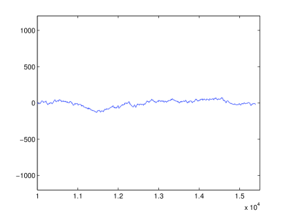
Figure 1: A typical crack of 500 growth steps in a.u. Note the difference in scales between the ordinate and the abscissa.

We have measured the roughness of the cracks in the model with both the variable bandwidth max-min method of Eq. (1) and the variable bandwidth RMS method 95SVR . In order to avoid strong finite size effects we have used the results of Ref. 95SVR to calibrate our results for the different measurement methods. This procedure turned up to be consistent in the sense that the variance in the results obtained by the different methods pointed to a single well-defined exponent according the finite size effects predicted in 95SVR . Finally, we averaged over different realizations, obtaining $\zeta=0.53\pm 0.03$. An example a single roughness measurement is shown in Fig. 2.

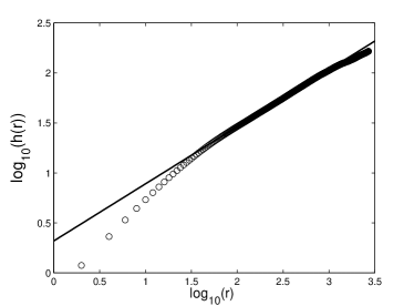
Figure 2: A log-log plot of the height fluctuations $h(r)$ of Eq. 1 as a function of the scale $r$. The straight line corresponds to $\zeta=0.57$.

This result indicates that the cracks in model B exhibit random roughness as the roughness exponent is not significantly different from the random walk exponent $\zeta=0.5$. This result is qualitatively different from the results of model A in which $\zeta=0.66\pm 0.03$. At this point we must conclude that even though the two models share many features and on the face apparently one should not expect dramatically different scaling properties, the two models belong to different universality classes. Model A exhibits correlated roughening, while model B exhibits random roughening. We turn now to further clarifying the origin of the qualitatively different results.

III.1 Common (and non-trivial) properties of models A and B

The first thing to point out is that both models A and B deviate from many models common in the literature in a way that might affect significantly the scaling properties. In both models the crack propagates via the nucleation and coalescence of damage at a finite distance $\xi_{c}$ ahead of its tip, essentially under the influence of a linear-elastic stress field. In ideal linear elasticity, the stress tensor field $\sigma_{ij}$ attains the following asymptotic form approaching the crack tip

$$\sigma_{ij}(r,\theta)=\frac{K_{I}}{\sqrt{2\pi r}}\Sigma^{I}_{ij}(\theta)+\frac{K_{II}}{\sqrt{2\pi r}}\Sigma^{II}_{ij}(\theta)\ ,$$ (9)

where $(r,\theta)$ is a polar coordinates system located at the crack tip, ${\bf\Sigma}^{I}$ and ${\bf\Sigma}^{II}$ are known universal functions and $K_{I}$ and $K_{II}$ are the stress intensity factors corresponding to opening (mode I) and shearing (mode II) stresses Lawn . Eq. (9) describes well the stress fields on a scale $r$ relative to the crack tip that is much smaller than any other length scale in the problem. Naturally, we cannot expect this formula to be precise for $r$ of the order of $\xi_{c}$. In particular, the hydrostatic tension $P(r)$ should be sensitive to significant corrections to the ideal law Eq. (9). We can expect that the stress fields on a scale $\xi_{c}$ away from the tip in both models is described by Eq. (9) with $K_{I}\gtrsim K_{II}$ plus additional terms. To verify this expectation we calculated the hydrostatic tension $P$ on an arc a distance $\xi_{c}$ from the tip and fitted to the form

$$P(\theta)=\ \frac{K_{I}}{\sqrt{2\pi\xi_{c}}}\left[\cos{\left(\frac{\theta}{2}\right)}+\frac{K_{II}}{K_{I}}\sin{\left(\frac{\theta}{2}\right)}\right],$$ (10)

predicted by Eq. (9) Lawn . The results support our expectation, showing that $K_{I}\gtrsim K_{II}$ and an additional contribution of 10-15% from other non-universal terms at a distance $\xi_{c}$ away from the tip for both models. An example is shown in Fig. 3.

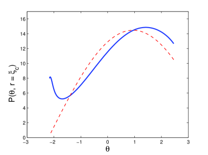
Figure 3: The hydrostatic tension $P$ (see Eq. 8) as a function of $\theta$ at a fixed radius $r\!=\!\xi_{c}$ (solid line) and a fit with $K_{I}\!=\!125~{}(a.u.)$, $\frac{K_{II}}{K_{I}}=-0.51$ (dashed line). The present data was taken from a crack after 300 growth steps, but it is representative.

The conclusion is that both models are in the non-linear regime (in terms of $K_{II}\{y(x)\}$). In addition one cannot neglect the influence of contributions on top of Eq. (9). We believe that this is an important aspect in the success of model A in reproducing a correlated roughening, quantitatively close to the experimental observations. It also explains why models which used the linear approximation of a straight crack plus a perturbed $K_{II}$ achieved scaling exponents different from those observed in experiments 06BPSa ; 97REF .

On the other hand, this cannot be the only factor explaining the results of model A since this feature is common to model B which fails to produce correlated roughening.

III.2 The difference between the models stems from the difference in randomness

We propose that the differences in randomness are responsible for the different universality classes of model A and B. Recall that the quenched disorder length $d$ in model B is of the order of the nucleation length $\xi_{c}$. As a result, there are only few weak points available for damage nucleation on a scale $\xi_{c}$. In this situation the crack “selects” a damage nucleation site out of a small number of possibilities and in fact there is a sizeable probability of having a growth step chosen uncorrelated with the deterministic field $P$ that carries the history of the evolution. We thus expect this randomization effect of uncorrelated growth steps to accumulate gradually and reduce the correlated roughening exponent observed in model A. The situation is fundamentally different in model A where the probability of having completely random growth steps is small. To support this explanation we have measured the roughness exponent $\zeta$ (see Eq. 2) as a function of the crack length in terms of growth steps. In Fig. 4 we show the dependence of $\zeta$ on the number of growth steps.

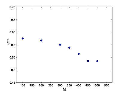
Figure 4: The average roughness exponent $\zeta$ as a function of the number of growth steps $N$.

It is observed that indeed roughness exponent $\zeta$ decreases monotonically from $\zeta\approx 0.625$ to $\zeta\approx 0.53$, presumably approaching asymptotically $\zeta\approx 0.5$. This finding is consistent with the suggested explanation.

IV Summary

We have studied the role of disorder in generating correlated roughening exponent in cracks of $1+1$ dimensions. The main conclusion is that adding additive material disorder to linear elasticity is not sufficient to generate correlated crack graphs with exponents larger than 0.5. This is due to the destructive events or uncorrelated steps which accumulate and gradually produce a random graph. The generation of correlated graphs ($\zeta>0.5$) is due to the correlations between the deterministic field (the hydrostatic pressure) and the pdf carrying the randomness, like the annealed disorder of model A. We reiterate the result concerning the magnitude of the stress intensity factors, and specifically $K_{II}$. The measurement of $K_{II}$ and higher order terms of the pressure field tells us that linear approximations of $K_{II}$, or the principle of local symmetry, do not represent properly the stress field at the vicinity of $\xi_{c}$ away from the rough crack tip. Therefore, one can view this feature as an additional test for models of crack growth which produce the observed correlated roughness.

- (1) E. Bouchbinder, I. Procaccia and S. Sela, Phys. Rev. Lett. 95, 255503 (2005).
- (2) J. Kertész, V.K. Horváth and F. Weber, Fractals, 1, 67 (1993).
- (3) T. Engøy, K.J. Måløy, A. Hansen and S. Roux, Phys. Rev. Lett, 73, 834 (1994).
- (4) L. I. Salminen, M.J. Alava and K.J. Niskanen, Rur. Phys. J. B. 32, 369 (2003).
- (5) E. Bouchbinder, J. Mathiesen and I. Procaccia, Phys. Rev. Lett. 92, 245505 (2004).
- (6) I. Afek, E. Bouchbinder, E. Katzav, J. Mathiesen and I. Procaccia, Phys. Rev. E 71, 066127 (2005).
- (7) E. Bouchaud and F. Paun, Comput. Sci. Eng., 1, 32 (1999).
- (8) E. Bouchbinder, J. Mathiesen and I. Procaccia, Phys. Rev. E 69, 026127 (2004).
- (9) L.D. Landau and E.M. Lifshitz, Theory of Elasticity, 3rd ed. (Pergamon, London, 1986).
- (10) N. I. Muskhelishvili, Some Basic Problems of the Mathematical Theory of Elasticity, (Noordhoff, 1953).
- (11) J. Lubliner, Plasticity Theory, (Macmillan, New York, 1990).
- (12) This way of representing disorder is different, for example, from lattice models in which a threshold taken from an uncorrelated distribution is assigned to each lattice point. In that case the disorder is not introduced by the fluctuations in the locations of weak points (as in our model B), but by the fluctuations in the breaking thresholds. For more information on lattice models, see H. J. Herrmann and S. Roux (Eds.), Statistical Models for the Fracture of Disordered Media, (North-Holland, Amsterdam, 1990).
- (13) J. Schmittbuhl, J.-P Vilotte and S. Roux, Phys. Rev. E 51, 131 (1995).
- (14) B. R. Lawn, Fracture of Brittle Solids 2nd Edition, (Camebridge University Press, 1998).
- (15) E. Bouchbinder, I. Procaccia and S. Sela, J. Stat. Phys.,in press (2006).
- (16) S. Ramanathan, D. Ertas, and D. S. Fisher, Phys. Rev. Lett. 79, 873 (1997).