Decoding Information from noisy, redundant, and intentionally-distorted sources

Abstract

Advances in information technology reduce barriers to information propagation, but at the same time they also induce the information overload problem. For the making of various decisions, mere digestion of the relevant information has become a daunting task due to the massive amount of information available. This information, such as that generated by evaluation systems developed by various web sites, is in general useful but may be noisy and may also contain biased entries. In this study, we establish a framework to systematically tackle the challenging problem of information decoding in the presence of massive and redundant data. When applied to a voting system, our method simultaneously ranks the raters and the ratees using only the evaluation data, consisting of an array of scores each of which represents the rating of a ratee by a rater. Not only is our appraoch effective in decoding information, it is also shown to be robust against various hypothetical types of noise as well as intentional abuses.

1 Introduction and Model

With the rapid advances in information technology, and especially the advent of the internet, information overload is becoming a growing challenge for our society. In fact, daily life and professional activities call for reliable information on a myriad of things, and no individual is capable of knowing it all. We can, at best, rely on other people’s evaluations to indirectly form an assessment on a subject or item that happens to catch our interest. Numerous web sites have already constructed evaluation systems which allow new users to benefit from the feedback of previous users ebay , E_commerce . However, even though many opinions can be found about any single object (be it a book, a product, an idea), they are frequently far from being consistent with each other, perhaps because people are of different expertise and/or have different levels of discernment. More often than not we are left without a clear, definite answer. This situation calls for automated methods of collaborative information filtering and ranking GroupLens .

Many web sites, which provide information filtering and evaluation for the general public, are themselves evaluated and ranked by all the individuals via perhaps other web sites. This self-organized selection has become increasingly popular among internet users and may play an important role in shaping the upcoming information-technology-mediated economics framework. Examples may be found through web sites such as del.icio.us, www.digg.com, www.reddit.com, www.tailrank.com et al. In a way, these sites all probe various selection and filtering mechanisms with varying degrees of success. We believe that it is time to examine the phenomena systematically in order to understand the theoretical foundation of information filtering.

In this work we formulate a prototype model to cope with such a challenge. Suppose $N$ users (raters) rate $M$ objects (ratees) in a given category. Each user has an idiosyncratic rating capability ($1/\sigma_{i}$ for rater $i$); each object has an intrinsic quality ($Q_{l}$ for object $l$). Both the rating capabilities and intrinsic qualities are assumed given and hidden. We wish to find estimates, $q_{l}$ and $V_{i}$, as close as possible to the hidden values, $Q_{l}$ and $\sigma_{i}^{2}$. Absent further information, people often use the simple arithematical average $q_{l}\equiv\sum_{i=1}^{N}x_{il}/N$ as the estimate for $Q_{l}$, where $x_{il}$ is the rating assigned by user $i$ to object $l$. With our additional assumption that users are of different rating capabilities, we may regard the rating $x_{il}$ as the sum of $Q_{l}$ and a stochastic component of typical size $\sigma_{i}$. Though many users report ratings on a given object, these signals can be termed noisy since there is no sure way to tell which evaluation is more reliable than the other. To make sense of these noisy signals our only hope is to leverage the information redundancy and find the best possible approximation to the hidden attributes.

As we will show below, the correctness of ranking can be distorted when the true quality of each object is estimated by the naïve simple average of that object’s ratings. This effect is amplified especially when the typical $\sigma_{i}$s vary significantly so that the simple average may be biased by raters with large $\sigma$s. Our method, termed iterative refinement, can nevertheless minimize the occurrence of this undesirable scenario.

2 Method

Our task is to simultaneously obtain good estimates $\{q_{l}\}$ and $\{V_{i}\}$ respectively for $\{Q_{l}\}$ and $\{\sigma_{i}^{2}\}$ using only the ratings $\{x_{il}\}$. Absent knowledge of $\{\sigma_{i}^{2}\}$, the simplest solution would be the naïve arithematical average $q_{l}={1\over N}\sum_{i=1}^{N}x_{il}$. Though it conforms to the principle of ‘one person one vote’, such a naïve average is often said to suffer from the ‘tyranny of the majority’, especially when the majority is poorly informed. When one knows $\{\sigma_{i}^{2}\}$, one can improve the accuracy of the prediction by giving more weight to experts with smaller $\sigma_{i}$s:

$$q_{l}=\sum_{i=1}^{N}w_{i}x_{il},$$ (1)

where $w_{i}=w(\sigma_{i})$ is a decreasing function of $\sigma_{i}$ and with the normalization condition $\sum_{i}w_{i}=1$. In fact, if the $w_{i}$ are properly chosen so that Lindeberg’s condition Feller holds, $q_{l}-Q_{l}$ becomes a zero-mean Gaussian random variable with variance $\propto 1/N$ when $N\to\infty$, thanks to the Lindeberg-Feller theorem Feller , Chung . Further, knowledge of $\{\sigma_{i}^{2}\}$ actually allows the determination of optimal choice Hoel for the weight $w_{i}\propto 1/\sigma_{i}^{2}$.

The problem, however, is that we know neither which are the best objects, nor who are the best raters. Nevertheless, since a better estimate of $\{\sigma_{i}^{2}\}$ will improve our estimate of $\{Q_{l}\}$, we have devised an iterative refinement method to simultaneously extract the raters’ rating capabilities and the objects’ intrinsic qualities. In particular, the rating capability of rater $i$ is estimated by

$$\sigma_{i}^{2}\approx V_{i}\equiv\frac{1}{M}\sum_{l=1}^{M}(x_{il}-q_{l})^{2}\;.$$ (2)

It is worth pointing out that due to error propagation (e.g. estimating $Q_{l}$ by $q_{l}$), equation (2) is not the best possible estimator of $\sigma_{i}^{2}$. Although it is possible to systematically compute all the correction terms by creating effective Gaussian variables through recombining random variables, we will not execute such a technique here to avoid unnecessary complications. The more technical optimization of the method proposed will be discussed in a forthcoming publication.

Assuming the weights to be of power-law type

$$w_{i}=\frac{1/V_{i}^{\beta}}{\sum_{j}1/V_{j}^{\beta}}\stackrel{{\scriptstyle q_{l}\to Q_{l}}}{{\Longrightarrow}}\frac{1/\sigma_{i}^{2\beta}}{\sum_{j}1/\sigma_{j}^{2\beta}},$$ (3)

equations (1) and (2) can be cast into a more suggestive form:

$$\sum_{i=1}^{N}{1\over{V_{i}^{\beta}}}(x_{il}-q_{l}) = 0,\;\;l=1,2,\ldots,M;$$ (4)

$$\sum_{l=1}^{M}{(x_{il}-q_{l})^{2}\over V_{i}} = M,\;\;i=1,2,\ldots,N.$$ (5)

The above construction is intuitively appealing especially when $\beta=1/2$. Assuming that the ratings fluctuate around the hidden qualities $Q_{l}$ with varying widths $\sigma_{i}$, the first equation is the sum of stochastic variables with a unique, normalized width, and the second sum defines the widths. On the other hand, the case $\beta=1$ intimately mimics the optimal weighting choice Hoel .

To solve for the $N+M$ unknowns using as many (nonlinear) equations is usually achieved by casting the problem as a minimization NR . This route is, in general, difficult for a nonlinear system because of the existence of multiple local minima that hinder the finding of the global one. When the equations are such that local minima rarely occur, finding the solution becomes a relatively straightforward numerical task. Fortunately, this is where our problem belongs. Our iterative refinement method starts with uniform weighting, then iterates eqs. (4,5) till convergence to the final solution with specified $\{q_{l}\approx Q_{l}\}$ and $\{V_{i}\approx\sigma_{i}^{2}\}$. Thus, we find simultaneously qualities of the ratees and raters.

As a cautionary note, we must comment that eq. (4) with $\beta=1/2$ takes a more gentle weight than suggested by the optimal weighting Hoel , which would recommend $\beta=1$. We choose a softer weighting scheme to start because it enjoys a better numerical stability, as well as translational and scale invariance – the equations remain the same upon changing $q_{l}\to c[q_{l}-g]$ and $x_{il}\to c[x_{il}-g]$. The better numerical stability for $\beta=1/2$ may be due to the fact that Lindeberg’s condition Feller is always satisfied there. Once the iterative procedure starts, the weighting scheme is then shifted from $1/\sigma$ towards $1/\sigma^{2}$ as the iterations progress. If the Lindeberg’s condition is satisfied for $1/2<\beta\leq 1$, this construction guarantees the convergence of $q$ towards $Q$ when each individual distribution function for $x_{il}$ is distinct but with a finite second moment, thanks to the Lindeberg-Feller Theorem Feller , Chung . As will be shown, the correct convergence is obtained even when the requirements leading to the general form of Law of Large Numbers are not satisfied, making our proposal far more general than the traditional proven domain.

3 Tests, results, and analysis

Before any rating system can be put into real use, it must at least pass theoretical quality control. The goal for a rating system is to produce the best approximation achievable, and to be robust against abuses and gaming attempts. Any proposed decoding scheme should undergo testing under controlled conditions (i.e. where $\{Q_{l}\}$ is known), whereas adaptation of a decoding method to realistic applications usually requires a leap of faith since $\{Q_{l}\}$ is unkonwn. In fact, we would never know what the hidden, intrinsic attributes are or their underlying distribution. A decoding method has a higher chance of success in the real world if it can consistently find the approximate hidden attributes with a high precision under a wide variety of controlled conditions. We try to choose, among infinite possibilities, a number of case-studies we deem most significant.

We assume the intrinsic qualities ($Q_{l}$ for object $l$) to be uniformly distributed and the ratings $x_{il}$ to be drawn from various individual distribution functions $P_{V}(x_{il})$, centered around $Q_{l}$ and characterized by different widths $\sigma_{i}$. This implies that the ratings from different users are assumed uncorrelated. Although we don’t plan to deal with this effect explicitly in this paper, we would like to point out that the correlation effect is automatically damped down when using our iterative refinement. Because we down weight users with weaker rating capabilities, sets of users with poorer rating capabilities but having correlated ratings will have their votes downweighted and therefore won’t be able to bias the result much. For users with excellent rating capabilities but having correlated ratings, keeping or removing the redundancy does not produce much effect on the final result either. The correlation between users, therefore, does not have a prominent effect. We will thus present the study of the correlation effect in a separate publication, and in the mean time return to the case of uncorrelated users.

To be specific, we shall employ the following voting distributions:

$$P_{V}(x_{il}) = {1\over\sqrt{2}\sigma_{i}}e^{-\sqrt{2}|x_{il}-Q_{l}|/\sigma_{i}}$$ (6)

$$P_{V}(x_{il}) = {(f-1)/2\over\sqrt{C_{f}\sigma_{i}^{2}/2}}\left({|x_{il}-Q_{l}|\over\sqrt{C_{f}\sigma_{i}^{2}/2}}+1\right)^{-f}$$ (7)

where $C_{f}=(f-2)(f-3)$ for $f>3$. In this case both distributions have finite second moments given by $\int P_{V}(x_{il})[x_{il}-Q_{l}]^{2}dx_{il}=\sigma_{i}^{2}$. We may extend the exponent $f$ to be in the range $1<f\leq 3$ at the expense of a divergent second moment, and set $C_{f\leq 3}=2$. The resulting distribution (7), falling outside the realm of the central limit theorem, will also be considered. Finally, the distribution widths $\sigma_{i}$ are also randomly drawn from a distribution function $p$. The broader the distribution function, i.e. the greater the inhomogeneity in rating capabilities, the harder it is to have resulting $q_{l}$’s close to the intrinsic $Q_{l}$’s.

As a quantitative measure of the accuracy of any estimation method, we use a Euclidean-like distance between the estimated solution $\{q_{l}\}$ and the intrinsic values $\{Q_{l}\}$:

$$\Delta=\sqrt{{1\over M}\sum_{l=1}^{M}(q_{l}-Q_{l})^{2}}.$$ (8)

Since in many applications it is required to rank the $M$ objects in order of decreasing quality, it is useful to compare the estimated ranked list $L_{E}$ with the intrinsic one $L_{I}$. A measure $I(p)$ is introduced to examine the ranking integrity within the top $p$ proportion of the object’s quality list:

$$I(p)\equiv{1\over[pM]}\sum_{R=1}^{[pM]}{n(R)\over R},$$ (9)

where $[x]$ indicates the maximum integer that is smaller than or equal to $x$. Here $n(R)$ denotes the number of objects, among the top $R$ ones in the estimated ranking list $L_{E}$, whose intrinsic qualities rank among the top $R$ in the intrinsic list $L_{I}$. The higher the quantity $I(p)$, the better the overlap between the estimated ranking and the intrinsic one. For illustrative purposes, we shall consider $p=0.5$ in this study. It is worth pointing out that the expectation value of $I(p)$ from random sampling can be calculated (see supplementary information for the complete proof):

$$\langle I(p)\rangle_{0}={[pM]+1\over 2M}\;\;\stackrel{{\scriptstyle M\gg 1}}{{\longrightarrow}}\;p/2;$$ (10)

In order to have a more precise measure of the variation of $\Delta$ and $I(p)$ around their respective means, we calculate the “up” variance $\langle(\Delta-\langle\Delta\rangle)^{2}\rangle_{\Delta>\langle\Delta\rangle}$ and “down” variance $\langle(\Delta-\langle\Delta\rangle)^{2}\rangle_{\Delta<\langle\Delta\rangle}$ (identically in $I(p)$ case) and report their square roots as asymmetric error bars in Figs. 1, 3 and 5.

Effect of the number of objects and raters

Both the distance measure $\Delta$ in eq. (8) and the ranking-integrity measure $I(p)$ in eq. (9) are functions of $M$ and implicitly of $N$. For simplicity we will assume $M=N$ and measure both $\Delta$ and $I(p=0.5)$ for various $N$ and different stochastic distribution functions $P_{V}(x)$.

As shown in Fig. 1.(a), using the iterative refinement method the difference between the $q$’s and the $Q$’s becomes smaller steadily with increasing $N$. When using the exponential distribution (6) for voting, within numerical errors the downward slope equals $-1/2$ as expected from the Law of Large Numbers. When the voting distribution function has a power law tail that prevents a finite second moment, the proposed method still shows steady improvement with increasing $N$. In Fig. 1.(a) we also show, as a comparison, the simple average with equal weights: the difference $\Delta$ is much larger and its convergence to zero is not guaranteed. Moreover, the precision for a moderately large set of data is strengthened by the rapid decrease of the error bars.

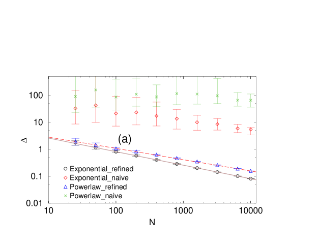
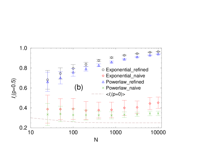
Figure 1.: Figures (a) and (b) show, respectively, the dependence of $\Delta$, from eq. (8), and of $I(p=0.5)$, from eq. (9), on the system size $N$. The intrinsic quality of each object is randomly uniformly drawn from the interval $(0,10)$. A small finite constant $\epsilon=0.001$ is introduced so that the judging width is always bounded by ${\rm const}/\epsilon$ to avoid the potential artifact of infinite width. For the power-law case (eq. (7)), we picked $f=2.5$, so that the second moment of $V$ diverges, to test the robustness of our method. Indeed, the deviations $\Delta$ still decrease steadily with size, although not as fast as for the exponential voting distribution (eq. (6)), while the ranking integrity grows. The solid (dashed) line passing through the exponential (power-law) voting distribution in graph (a) has slope $-0.50\pm 0.01$ ($-0.42\pm 0.01$). The dashed line in graph (b) is the result for the random case (eq. (10)). Error bars have been estimated from the standard deviation of one hundred realizations of different initial configurations.

In Fig. 1.(b) we show how the ranking integrity changes with size. There is a clear separation between the naïve arithematical average and the iterative refinement method. The increase of the ranking integrity with $N$ confirms that the robustness of our method increases steadily with the system size. When using the naive averages, on the other hand, it seems to change only slightly or not at all, within the precision of the indicated error bars.

Self-evaluating community

Our method can be easily applied to another context: a self-evaluating community. Suppose a community of experts tries to find the intrinsic ranking of its own membership. Each expert has an opinion on every other member in this community and opinions are uncorrelated. In this case we have $N=M$ and the asymmetrical matrix element $\{x_{ij}\}$ denotes $i$th member’s rating on $j$th member. Thus, each member has a given attribute we call quality as well as a given rating capability. With minor modifications, (4) and (5) become

$$\sum_{i\neq j}{1\over{V_{i}^{\beta}}}(x_{ij}-q_{j}) = 0,\;\;j=1,2,\ldots,N\;,$$ (11)

$$\sum_{j\neq i}{(x_{ij}-q_{j})^{2}\over V_{i}} = N,\;\;i=1,2,\ldots,N\;.$$ (12)

Our iterative approach can be readily used to find the solutions for the $q$’s and the $V$’s (estimated for $Q$’s and $\sigma^{2}$’s). There are members who are judged by others as higher quality authorities and some members turn out to excel at rating fellow members. Still others are good at both.

For the self-evaluating community, the simulation results on $\Delta$ and $I(p=0.5)$ largely agree with those presented in Fig. 1. Apparently, one may wishfully believe that there exist correlations between the qualities of being good experts and being good raters. For example, in the real world people often assume that being a good expert automatically implies being a good rater. However, we should be cautious in this regard: though very likely the two types of quality are somewhat correlated, we should let the data itself bring out evidence which may support or undermine such a hypothesis. To demonstrate this possibility, we have run a simulation where everyone has the same rating capability and another where the rating capability $1/\sigma_{i}$ of user $i$ is directly proportional to his quality $Q_{i}$ of being a good expert. Although no information about the correlations between $Q_{i}$ and $\sigma_{i}$ is fed into our iterative refinement method, the result shown in Fig. 2. – plotting $1/V^{1/2}$ versus $q$ – reflects strongly the respective underlying correlations.

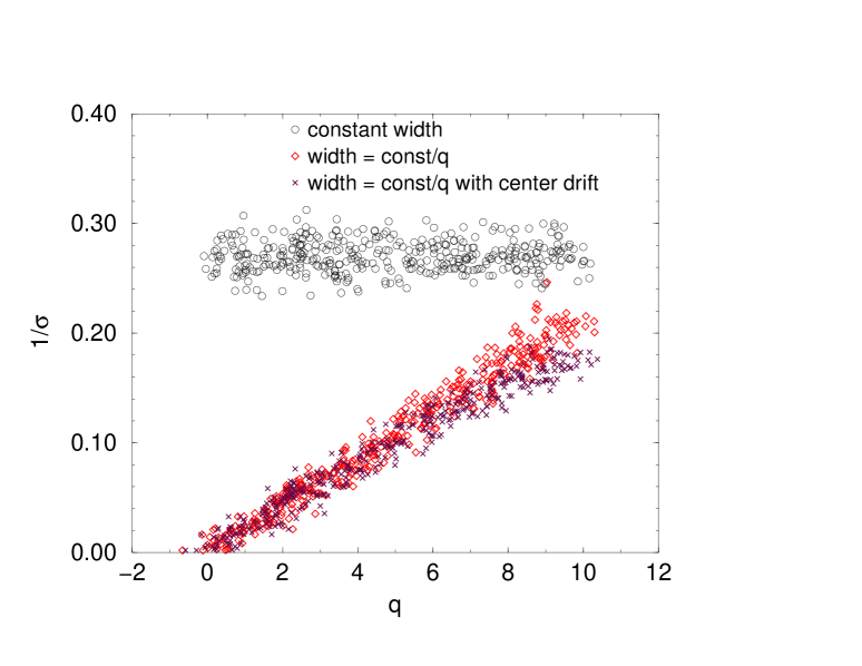
Figure 2.: Experts’ estimated rating capability versus estimated quality. Using $N=400$, data is taken from the outcome of a typical single run with, respectively, $\sigma_{i}={\rm const.}$ (circles), $\sigma_{i}={\rm const.}/Q_{i}$ with a random center-drift uniformly distributed between $[-5,5]$ (x signs) and without drift (diamonds).

Individualized biases of the target $Q_{l}$

One may object to the fact that each rater’s distribution is symmetrical around the intrinsic attribute. To subject our method to more severe tests, we now relax this condition: we allow each rater to have an individual distribution function not only with a specific width, but also an object-dependent individualized biased center. Thus, $x_{il}$ is drawn around $Q_{l}+\Delta Q_{il}$, where the center drift $\Delta Q_{il}$ represents the individual bias.

For testing purposes, the quantity $\Delta Q_{il}$ was drawn from a uniform distribution inside $[-5,5]$, while the intrinsic qualities $Q_{l}$ are within the range $[0,10]$. Despite the fact that $\Delta Q$ has a rather large range, the convergence of $q$ to $Q$ is almost as good as in the unbiased case. There is only a small increase in $\Delta$ and a negligible decrease in $I(p=0.5)$. Even in the case of the self-evaluating system, the modification does not spoil the underlying characteristics. As shown in Fig. 2., when the rating capability is directly proportional to the expert quality, the linear relationship found between $1/V^{1/2}$ and $q$ still holds, except with a smaller slope.

We may conclude that the proposed method is quite effective in decoding the hidden attributes in the controlled numerical experiments. However, before proposing it for real applications we must face another type of challenge: members may harbor private agendas and may willfully distort information. So far we have dealt with random, neutral noise, which we shall call the first kind. The second kind of noise, is unique for intended human actions. Comparing with the information theory of Shannon for transmitting signals via a noisy channel shannon , which by definition deals with noise of the first kind, we must be wary that our method should be relatively robust against willful distortion as well. As people often observe in real life information collection and evaluation, gaming the system is often hard to detect, and still harder to stop. We now turn to this case.

Intentional distortion

Consider the context of a mutually evaluating community. Since friendships and rivalries are as ancient as civilization in any human grouping, we must expect that some will give a more favorable evaluation for their friends, with upward deviations often larger than what their rating capability would warrant. Likewise they may rate down their enemies. For this reason we shall extend the proposed model to include some friendship-enemy pairs among the members of the community. A simple way to implement this is to pick in turn every member, sending out a fixed number of friendly links landing randomly on fellow members, and the same number of enemy links. As a result of this procedure, any member can receive more or less friendly or hostile links. When two members are linked by a friendly link, they trade favors by up-rating each other by a upwards bias. Likewise, two enemies will rate down each other by a downward bias. To simulate this effect, when a member $i$ votes on his friend (enemy) $j$, we increase (decrease) the vote $x_{ij}$ by $2\sigma_{i}$. As a control parameter we denote by $\gamma$ the percentage of friendly and hostile links. For instance, at $\gamma=30\%$ each member has $30\%$ out of the total fellow members as friends, and as many enemies. Thus, the remaining $40\%$ are neutral ones to him.

In Fig. 3. we see that, as the percentage $\gamma$ increases, i.e. the community becomes more and more corrupted and ratings become less and less fair, the decoding efficiency deteriorates. Specifically, one should note the increase of $\Delta$ and the decrease of $I(p=0.5)$ as $\gamma$ increases. However, the overall efficiency holds remarkably well in the face of the massive information corruption. Even when the majority of fellow members are either friends or enemies, the solution $q$ still remains very close to $Q$. As a comparison, we see that the ranking integrity from the simple average quickly worsens and comes close to the expectation value from informationless random sampling.

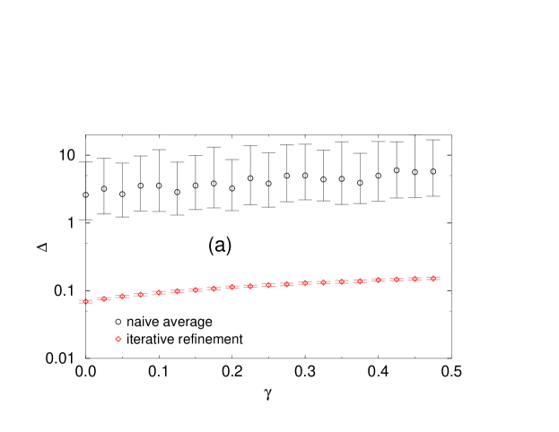
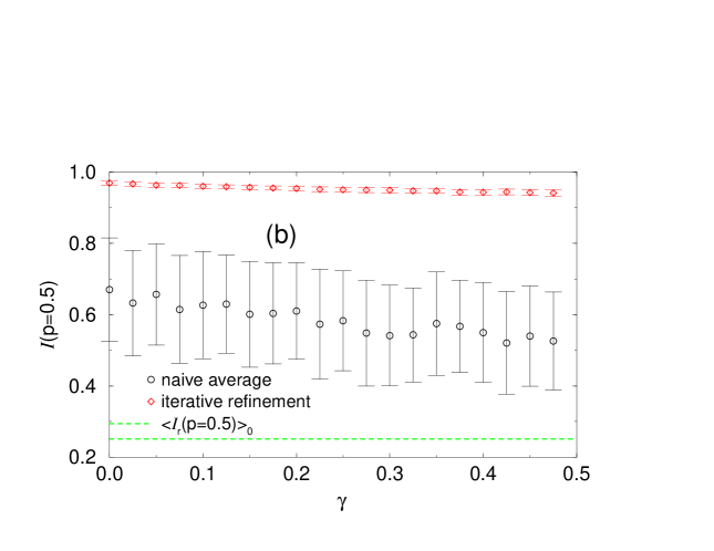
Figure 3.: The effect of intentional distortion on $\Delta$. The abscissa records $\gamma$, the ratio of friends and enemies to the population in a community; the ordinate documents the distance $\Delta$ (a) and the rank integrity $I(p=0.5)$ (b). Using $N=400$, the data are obtained from the outcome of one hundred simulation runs. The standard deviations from the mean value are shown as a vertical bar around the average value.

When a member rates another member far away from the intrinsic attribute, the mischief costs him somewhat in credibility $1/V^{1/2}$, which is the estimate of his rating capability $1/\sigma$. If there are a high fraction of friends and enemies, then all are adversely affected in their rating capabilities; this is best seen from Fig. 3.(b), which shows how the ranking integrity worsens as the friend/enemy fraction $\gamma$ increases.

Stability against worst abuses

It is instructive to examine the maximum ability for a member to willfully distort information about another. We would like to investigate the effect of a willful distortion on the final rating of the targeted member as well as on the cheater’s estimated rating capability, which can also be interpreted as his credibility within the community. For this purpose, the simplest method is to consider a fair community, where only one member harbors a hidden agenda to distort the rating of another member by a very wide margin. Since all other raters are fair, the impact of this distortion can be calculated, as well as the repercussion on his own rating capability, judged by the community. If the cost is high for the cheater compared to the possible impact the cheating would have, then we may conclude that the method is naturally robust in constraining cheating behavior; if the cost is low for a similar impact, we should expect that cheating would run rampant and additional features are called for to prevent it.

It is practical to represent all the members in two rank lists: one for their quality judged by the fellow members; another for their rating capability as the result of their behavior in judging others. This is similar in spirit to the notion of authority and hub Kleinberg , two qualities that are also central in ranking web pages. Assume one cheater in an otherwise fair community. Because promotion and demotion have almost identical costs on the cheater’s rating capability, we need illustrate in detail only one of the two possible ways of cheating. Suppose the cheater promotes a friend beyond the intrinsic merit by a quantity $B$. We wish to know ($i$) by how much this promotion would move his friend up in the attribute rank list, and ($ii$) by how much this cheating would move the cheater down on the rating capability rank list. We may further inquire what is the maximum distortion a member can possibly create. This is interesting since only by knowing the worst case scenario can we learn how robust this method is.

First we note that there indeed exists an upper bound on the possible cheating. A member launching a desperate distortion act, not caring about any damage to his own rating capability, could not favor his fellow indefinitely. Because the rating from cheater $I$ is weighted by $1/V_{I}^{{\beta}>1/2}$ (see the METHOD section) and $V_{I}(B\gg 1)$ is related to $V_{I}(B=0)$ via the relation

$$V_{I}(B\gg 1)-V_{I}(B=0)=\frac{B^{2}}{N}[1+\mathcal{O}(1/B)],$$

the overall contribution from cheater $I$ on his pal $J$ that he is trying to promote behaves like

$$\approx{x_{IJ}+B\over[\sigma_{I}^{2}(B=0)+\frac{B^{2}}{N}]^{\beta}}$$

for large $B$, and it becomes vanishingly small when $\beta>1/2$. This indicates that when rating an object way out of proportion, the net effect is as if the distorted vote never existed and our desperate cheater may not want to inflict such an egregious distortion lest his credibility drops to the bottom of the list. Such a desperate act in reality inflicts the maximal damage to his own credibility while achieving little desired result. Therefore, a rational cheater may then take a more calculated approach to produce a maximal distortion. A highly credible member can generate a larger distortion than an average member, should he choose to do so; a member on the bottom of the rating capability rank list has, however, weaker impact on promoting or demoting other members.

From the system point of view, we do not have to suffer from the maximal distortion. It is easy to detect such attempts and the cheater’s rating can be simply ignored and, at our discretion, the cheater’s rating capability can be restored since his contribution evaluating other neutral members is a valuable service we want to keep. We call this the “S” strategy. The implementation of the “S” strategy is flexible, we can either choose to inflict a punitive penalty or simply detect cheating and ignore it. Although it should depend on how reliably we can detect cheating, we currently implement the “S” strategy in two steps: if the rating from voter $i$ to object $l$ is more than two $\sqrt{V_{i}}$ away from $q_{l}$, we down weight the rating $x_{il}$ by an additional factor $(2\sqrt{V_{i}}/|x_{il}-q_{l}|)^{1/2}$ and we totally discard the weight whenever $|x_{il}-q_{l}|>3\sqrt{V_{i}}$.

A simulation of $400$ experts in a self-evaluating community is performed to test the effect of intentional distortions. In this simulation, we assume that each rater’s rating capability is directly proportional to his intrinsic quality. Forty realizations of different rating matrices are evaluated with the iterative refinement approach and the rank changes due to cheating for each rating matrix are averaged. We note that, as summarized in Fig. 4.(a), when the cheater’s intrinsic rating capability ranks high, he can promote others more than a cheater with mediocre rating capability. The cheater will have to pay a price of moving his rank down on the rating capability list by about $100$ to achieve the maximum distortion of about $10-15$. However, once we turn on the “S” strategy, appreciable distortion can no longer be achieved, as demonstrated in the bottom two curves of Fig. 4.(a). Therefore, it is possible to maintain a high degree of fairness and discourage cheating when this new method is employed in real society. With more information shared and less cheating allowed, our society can grow into a happier and healthier whole.

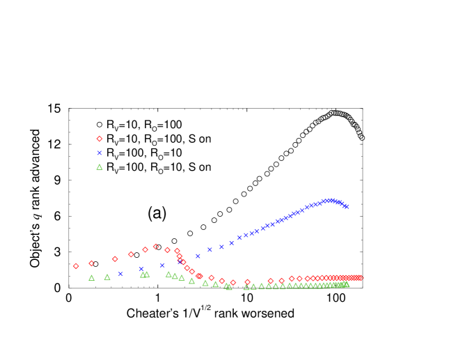
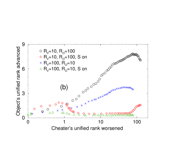
Figure 4.: The effect of extreme intentional distortion on the object’s rank (a) and on the object’s unified rank(b). ${\sf R_{V}}$ represents the cheater’s rank in the intrinsic rating capability list, while ${\sf R_{O}}$ represents the benefited object’s rank in the intrinsic quality list. By increasing the amount of intentional distortion $B$, the $1/\sqrt{V}$ rank of the cheater worsens while the $q$ rank of the benefited object also covaries. When the “S” strategy is turned on, we see that the cheater has very little impact in distortion, despite how willing he is to sacrifice himself. See the text for the explanation of the final bump in the red curve of figure (b).

In real life the rating capability and one’s intrinsic quality might not be always correlated, as plausibly assumed in our simulation. However, without any presumption, working with real data may well reveal any correlation, since the method we propose does not exclude any specific one. We may propose a combined quality parameter to represent a member’s overall capability, $q/\sqrt{V}$. Any member, found to rank high on this new combined rank list, will be both judged highly by fellow members and behave well in judging others. The new rank list would also serve as a deterrent to cheating: any willful distortion attempt would cost a cheater somewhat in overall quality. The cost-benefit analysis now becomes even simpler: cheating may move up (down) a friend’s (enemy’s) rating, but the cheater’s own overall rating slips. In the previously mentioned simulation, we also document the change of this unified rank for both the cheater and the benefited object. In Fig. 4.(b) it appears again that cheating does not pay. Note that the bump in the tail of ${\sf R_{V}=10,\leavevmode\nobreak\ R_{O}=100}$, with strategy “S” turned on, is not an indication of the malfunction of our method. In fact, there the advance of the object’s unified rank is due to the fact that the cheater’s unified rank has dropped below that of the object’s. This nice feature again discourages severe cheating!

Finally, one may also wish to test the method against the possibility of ignorant voters. To model this, we assume there is only a certain proportion $C$ of the raters voting according to distribution (6), while the rest of the raters are voting randomly between $\epsilon$ and $10+\epsilon$. Figure 5. documents the test using a population of $400$ voters in a self-evaluating community. Our method provides appreciable improvement over the simple average

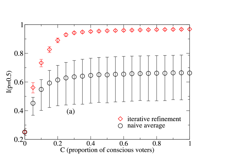
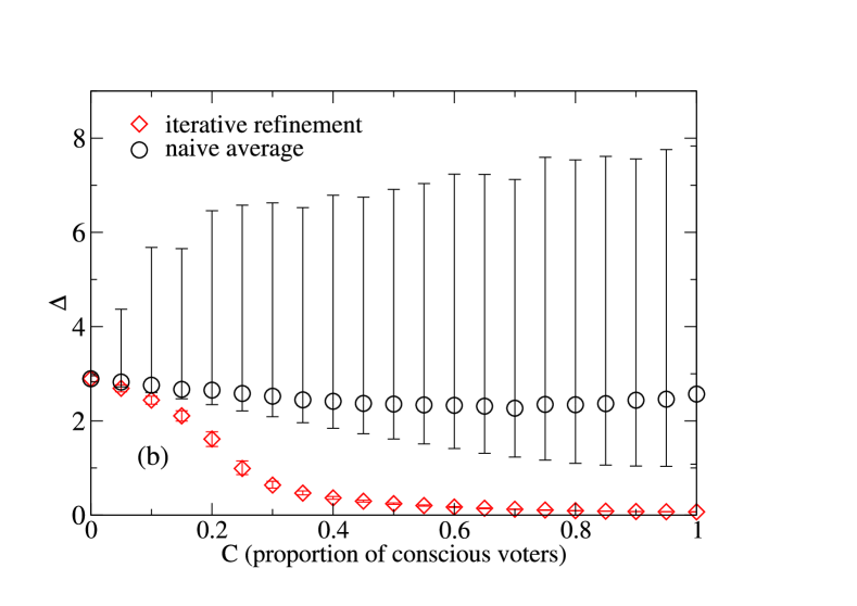
Figure 5.: The effect of ignorance. $C$ represents the proportion of conscious raters who vote according to the exponential distribution (6). (a) Ranking integrity $I(p=0.5)$ against $C$. (b) $\Delta$ against $C$. We see that $I(p=0.5)$ (resp. $\Delta$) increases (decreases) rapidly, and becomes much bigger (smaller) than the simple average, when $C>0.4$. $\sigma$’s of conscious voters are drawn from an exponential distribution with mean $1$.

4 Outlook and Concluding Summary

We have proposed an iterative refinement method to estimate the hidden intrinsic qualities of a set of objects that have been evaluated by a group of raters. The method consists of aggregating these evaluations in a weighted sum, with the aim to give more weight to expert raters. Weights and qualities are estimated iteratively from the same data set. Extensive simulation results show that the proposed method is able to recover the hidden attributes with remarkably good precision, even when the conditions of the Law of Large Numbers are not fulfilled. In particular, it overwhelms the performance of the naive simple average in most circumstances.

The proposed method is intended to be mainly applied to virtual communities of all kinds, where people are allowed to express their opinions on a particular subject –which can be a material object, a person or even another opinion. In addition to the objects’ intrinsic values, the method allows detection of the rating capabilities of the users. This provides valuable information, since it defines reputations manifesto without the need of any other feedback. It may constitute a strong incentive for users to rate accurately the desired object and a strong deterrent against cheating.

In fact the proposed method is robust against gaming. It remains effective in decoding the hidden attributes in the face of two types of noise: random and intentional. Although we fully anticipate this approach to be effective when working on real data where the intrinsic values $\{Q_{l}\}$ are not known at all, we are in the process of making more critical assessments by gathering data from existing web sites and by even designing special purpose web sites to acquire custom data. With more information shared and less cheating allowed, we hope our method, once implemented, can help our society to grow into a happier and healthier whole.

Appendix

In this appendix, we will derive the formula shown in eq. (10). Consider we have $M$ objects, labeled by $O_{1},\leavevmode\nobreak\ O_{2},\leavevmode\nobreak\ \ldots,O_{M}$, and we randomly put them into an ordered array of size $M$. Apparently, there are $M!$ ways to do so. The question is then to obtain the probabilities $P(k|\ell)$ for $k$ objects out of $O_{1},\leavevmode\nobreak\ O_{2},\leavevmode\nobreak\ \ldots,O_{\ell}$ to be in the top $\ell$ entries of the array.

When $k=\ell$ we only have $\ell!$ ways to order these $\ell$ objects and $(M-\ell)!$ ways to arrange the rest. Therefore, when $k=\ell$, we have $P(\ell|\ell)=(M-\ell)!\ell!/M!$. When $k<\ell$, we have to put $(\ell-k)$ objects in the lower $M-\ell$ bins and $k$ objects in the top $\ell$ bins. There are $(M-\ell)!/(M-2\ell+k)!$ ways for the former and $\ell!/(\ell-k)!$ ways for the latter. Further, there are ${\ell!\over k!(\ell-k)!}\equiv C_{k}^{\ell}=C_{\ell-k}^{\ell}$ ways to choose which $k$ objects to put in the top $\ell$ bins. Consequently, we have

$$P(k|\ell) = {(M-\ell)!\over M!}{\ell!\over(\ell-k)!}C_{k}^{\ell}{(M-\ell)!\over(M-2\ell+k)!}$$ (13)

$$= {1\over C_{\ell}^{M}}C_{k}^{\ell}C_{\ell-k}^{M-\ell}.$$

As a simple check, we can verify that $\sum_{k=0}^{\ell}P(k|\ell)=1$ because $\sum_{k=0}^{\ell}C_{k}^{\ell}C_{\ell-k}^{M-\ell}=C_{\ell}^{M}$ which can be easily proved by evaluating the coefficient of $x^{\ell}$ in the two equivalent expressions $(1+x)^{M}$ and $(1+x)^{M-\ell}\times(1+x)^{\ell}$.

It is instructive to compute the expectation value of $k/\ell$ for a given $\ell$

$$\left\langle{k\over\ell}\right\rangle = \sum_{k=0}^{\ell}{k\over\ell}C_{k}^{\ell}C_{\ell-k}^{M-\ell}=\sum_{k=1}^{\ell}C_{k-1}^{\ell-1}C_{(\ell-1)-(k-1)}^{(M-1)-(\ell-1)}$$

$$= \sum_{k^{\prime}=0}^{\ell-1}C_{k^{\prime}}^{\ell-1}C_{k^{\prime}-(\ell-1)}^{(M-1)-(\ell-1)}=C_{\ell-1}^{M-1}$$

Now the quantity of interest $I(p)$, averaged under a random ensemble, can be expressed as

$$\langle I(p)\rangle_{0}={1\over[pM]}\sum_{\ell=1}^{[pM]}{C_{\ell-1}^{M-1}\over C_{\ell}^{M}}={1\over[pM]}\sum_{\ell=1}^{[pM]}{\ell\over M}={[pM]+1\over 2M}$$ (14)

References

- [1] Laureti, P., Slanina, F., Yu, Y.-K., Zhang, Y.-C. (2004) Physica A, 316, 413-429.
- [2] Guttman, R.H., Moukas, A.G., Maes, P. (2001)The Knowledge Engineering Review, Cambridge University Press, New York.
- [3] Newman, M.E.J. (2001)Who is the best connected scientist? A study of scientific coauthorship networks, Phys.Rev. E64, 016131
- [4] Resnick, P., Iacovou, N., Suchak, M., Bergstrom, P., Riedl, J. (1994) CSCW (Proceedings of the 1994 ACM conference on Computer supported cooperative work), pp.175-186, October 22-26, 1994, Chapel Hill, North Carolina, United States
- [5] Shannon, C.E. (1949) The mathematical theory of communication, University of Illinois Press.
- [6] Kleinberg, J.M. (1999) Journal of the ACM, 46 604-632.
- [7] Masum, H., Zhang, Y.-C. (2004) Firstmonday, 9, (7)
- [8] Barabasi, A.-L., Albert, R., Jeong, H. (1999) Mean-field theory for scale-free random networks, Physica A, 272, 173-187
- [9] Feller, W. (1971) Introduction of Probability Theory and Its Applications, John Wiley & Sons, New York, Vol.II, 2nd ed., Chap. VIII.
- [10] Chung, K.L. (1968) A Course in Probability Theory Harcourt, Brace & World, New York, Chap. VII.
- [11] Hoel, P.G. (1983) Introduction to Mathematical Statistics John Wiley & Sons, New York, 5th Ed., pp.126-127.
- [12] Press, W.H., Teukolsky, S.A., Vetterling, W.T., Flannery, B.P. (1997) Numerical Recipe in C Cambridge University Press, Cambridge, 2nd Ed.
- [13] Albert, R., Barabási, A.-L. (2002) Statistical mechanics of complex networks Rev. Mod. Phys., 74 47.
- [14] Park, J., Newman, M.E.J. (2005) A network-based ranking system for American college football, Journal of Statistical Mechanics, (P10014)