The Mott insulator phase of the one dimensional Bose-Hubbard model: a high order perturbative study

Abstract

The one dimensional Bose-Hubbard model at a unit filling factor is studied by means of a very high order symbolic perturbative expansion. Analytical expressions are derived for the ground state quantities such as energy per site, variance of on-site occupation, and correlation functions: $\langle\hat{a}_{j}^{\dagger}\hat{a}_{j+r}\rangle$ and $\langle\hat{n}_{j}\hat{n}_{j+r}\rangle$. These findings are compared to numerics and good agreement is found in the Mott insulator phase. Our results provide analytical approximations to important observables in the Mott phase, and are also of direct relevance to future experiments with ultra cold atomic gases placed in optical lattices. We also discuss the symmetry of the Bose-Hubbard model associated with the sign change of the tunneling coupling.

I Introduction

One of the most fascinating recent trends in physics of cold gases concerns atomic gases in optical lattices jaksch ; bloch ; esslinger . These systems offer “atomic Hubbard toolbox” annals that can be used for studies of condensed matter models in a uniquely controlled manner. Cold atoms in optical lattices can be used for investigation of high $T_{c}$ superconductivity hightc , disordered systems sanpera , various spin models duan , novel quantum magnets bodzio1 , etc. Perhaps the most important version of the Hubbard model, that can be studied in optical lattices, is the Bose-Hubbard model (BHM) fisher . This model is a prototypical system on which understanding of quantum phase transitions (QPTs) in boson systems is based sachdev , and it has important applications in construction of a quantum computer qc .

Despite lots of theoretical studies on the BHM dmrg ; qmc ; krauth ; white ; batrouni ; elstner , there is still lack of analytical predictions about some basic experimentally relevant quantities. This motivates us to present here the results of a high order perturbative expansion in the tunneling coupling. These results, providing analytical approximations to different physical quantities in the Mott phase, should be helpful in the interpretation of experimental data.

We focus on a one dimensional (1D) homogeneous system at average density of one atom per site, i.e., on the simplest BHM undergoing a QPT. We calculate the following ground state quantities: energy per site ${\cal E}$, atom-atom correlations $C(r)=\langle\hat{a}_{j}^{\dagger}\hat{a}_{j+r}\rangle$, density-density correlations $D(r)=\langle\hat{n}_{j}\hat{n}_{j+r}\rangle$, and variance of on-site number operator ${\rm Var}(\hat{n})=[\langle\hat{n}_{j}^{2}\rangle-\langle\hat{n}_{j}\rangle^{2}]^{1/2}$.

The Hamiltonian of interest, in terms of dimensionless variables used through the paper, reads

$$\hat{H}=-J\sum_{i=1}^{M}(\hat{a}_{i+1}^{\dagger}\hat{a}_{i}+{\rm h.c.})+\frac{U}{2}\sum_{i=1}^{M}\hat{n}_{i}(\hat{n}_{i}-1),$$ (1)

where we denote the number of atoms, and the number of lattice sites as $M$. Since physics of the BHM depends on the $J/U$ ratio only, we set $U\equiv 1$ for convenience. With this choice, the critical point between the Mott insulator (MI) ($0\leq J<J_{c}$) and superfluid (SF) ($J>J_{c}$) is at $J_{c}\approx 0.29$ white .

Though the great deal of attention was recently devoted to cold atoms in inhomogeneous lattices bloch ; esslinger ; batrouni , the homogeneous systems described by the Hamiltonian (1) can be realized in the nearest future in at least two setups. First, there is a recent experiment done in the Raizen group raizen , where a single, one dimensional, homogeneous box is realized in a proper configuration of laser beams. After superposing a standing laser field on it, a 1D homogeneous Bose-Hubbard model (1) with open boundary conditions can be achieved. Since it was already demonstrated in raizen that one can load this 1D box with ultracold bosons and then count them very efficiently, the studies of lattices with a desired number of atoms per site should be available (as discussed below on specific examples). Another experimental opportunity shows up after realization of the ring-shaped optical lattice proposed recently in Ref. osterloh . This time, a 1D homogeneous lattice with periodic boundary conditions should be available for experimental investigations.

II The method

Our findings come from a high order symbolic perturbative expansion in the tunneling coupling. This method was first successfully applied to the calculation of a ground state and excited states of the BHM in one and two dimensional systems by Elstner and Monien elstner . We compare perturbative expansions to numerical data obtained using the imaginary time evolution with the so-called Vidal’s algorithm Vidal , which is equivalent to Density Matrix Renormalization Group scheme collath . This allows for verification of accuracy of our analytical predictions. The Vidal’s algorithm calculations assume open boundary conditions, which breaks the translational invariance of the system. To minimize finite size effects during comparison between the numerics and perturbative expansions valid for infinite systems (where boundary conditions are irrelevant) we have calculated the correlation functions around the system center.

We aim at calculation of high order perturbative corrections to different quantities of interest in the infinite Bose-Hubbard model. The perturbation theory is developed around the Fock state $|1,1,\dots\rangle$, where the numbers are boson on-site occupations. The expansion is done in the $J$ parameter (1).

In principle, the calculations can be performed by hand by perturbative determination of the wave-function up to a given order in the infinite system, and then subsequent calculation of expectation values in this wave-function. The attainable order of the expansion, however, is very limited (the wave-function can be determined up to the $J^{3}\sim J^{4}$ terms) so this method is not an option here.

A better alternative is to perform a linked cluster expansion (LCE) gelfand that has been used so far in spin systems spins and the Bose-Hubbard model elstner . This method consists of two steps. First, one has to generate all the clusters (sets of lattice sites in the BHM elstner ) that contribute to a given order of expansion. The largest of these clusters have the size comparable to the order of expansion. Then, one has to perform a perturbative expansion in the relevant clusters and sum up the results properly. In the end, one gets perturbative expansion of different quantities valid for infinite system from analysis of finite clusters. Since the whole procedure can be implemented on a computer in a symbolic way, the high order expansions become feasible.

The key for our calculations message from the LCE is the following: all the information about $i$-th order perturbative expansions in the infinite system is encoded in the small subsystems of the size $\sim i$. In accordance with this statement, we observe for every non-extensive observable that we consider, say $O$, that when we do a perturbative expansion $O|_{M}=\sum_{i}O_{i}|_{M}J^{i}$ ($M$ is the system size) the following holds

$$O_{i}|_{M}\equiv O_{i}|_{M_{c}},\ \ M\geq M_{c}(i),$$ (2)

i.e., the perturbative corrections become size independent for large enough systems. Naturally, $M_{c}(i)$ grows with $i$, but the growth is “reasonably” slow: $M_{c}(i)\sim i$ (see Table 1). We can not, of course, check explicitly the relation (2) for arbitrarily large $M$, but it is clear from the LCE that the size independent expansion terms ($O_{i}|_{M\geq M_{c}}$) correspond to infinite system predictions.

In our calculations we make a direct use of the relation (2) avoiding therefore generation of the cluster states. This simplifies the computer implementation of the whole procedure, but probably leads to more stringent requirements on the computer resources. To be more specific, we fix the system size $M$, assume periodic boundary conditions to keep the system translationally invariant, and do a standard perturbative expansion leading to determination of the ground state wave function up to a given order (Appendix A). Having the ground state wave-function, we calculate perturbative corrections to the expectation values of different operators and study their dependence on the system size $M$. This way we easily get $M_{c}(i)$ that guarantees (2): Table 1, as well as the desired perturbative corrections valid for infinite systems. Notice that due to (2) all finite size contributions are filtered out from the perturbative expansions for large enough $M$. To illustrate these findings we note that the 2nd order correction to the ground state energy per site in 3 sites and 3 atoms system is the same as in the infinite model at unit filling factor – a result that can be easily verified analytically.

${\cal E}$	$C(r)$	$D(r)$
$M\geq i+1$	$M\geq i+1+r$	$M\geq i+1$ and $2r\leq i$

Table 1: Conditions on the system size $M$ for getting size independent perturbative predictions at $i$-th order to ${\cal E}$, $C(r)$ and $D(r)$ – see (2). These results are obtained for the system filled with one atom per site.

III Perturbative expansions

To start, the ground state energy per site, ${\cal E}$, satisfies

$$\frac{{\cal E}}{4} =-J^{2}+J^{4}+\frac{68}{9}J^{6}-\frac{1267}{81}J^{8}+\frac{44171}{1458}J^{10}-$$ (3)

$$\frac{4902596}{6561}J^{12}-\frac{8020902135607}{2645395200}J^{14}+{\cal O}(J^{16}).$$

Before proceeding further, it should be stressed that the fractions come from a symbolic calculation, whose details are presented in Appendix A.

Coming back to (3), we notice that so far the largest published order of ${\cal E}$ expansion was the sixth elstner . Naturally, the expansion of ${\cal E}$ from elstner matches first three terms of (3). Changing fractions into numbers one gets approximately the following sequence of non-zero coefficients $\{-1,1,8,-16,30,-747,-3032\}$, which shows that the series has a rather unpredictable form.

To estimate accuracy of the expansion we plot (3) vs. numerical data for a fairly large system of $40$ atoms in $40$ sites: Fig. 1. This plot shows that there is quite a good agreement between (3) and numerics for $J$ smaller than about $0.3$, i.e., at least in a MI phase. The discrepancies present in Fig. 1 (and all other figures in this paper), may come from the following sources. First, our numerics is done in a finite system with open boundary conditions, while perturbative expansion yields results for infinite system. Second, we might need more expansion terms to get more accurate predictions. Third, the full perturbative expansion may fail to converge for large enough $J$’s, probably $J\geq J_{c}$. In the worst case, the series might be of asymptotic kind as was shown to be the case in some other systems zin . Further discussion about convergence of expansions presented here is beyond the scope of the present contribution.

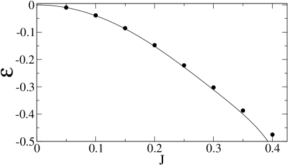
Figure 1: The perturbative prediction for the ground state energy per site from (3) (solid line) vs. numerics for $M=40$ system (dots).

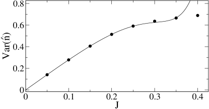
Figure 2: The perturbative result for the variance of on-site number operator from (4) (solid line) vs. numerics for $M=40$ system (dots).

The variance of on-site number operator, ${\rm Var}(\hat{n})$, up to ${\cal O}(J^{15})$ terms satisfies

$$\frac{{\rm Var}(\hat{n})}{\sqrt{2}} = 2J-3J^{3}-\frac{1441}{36}J^{5}+\frac{32045}{648}J^{7}-\frac{3105413}{5184}J^{9}$$ (4)

$$+ \frac{6979423019}{839808}J^{11}+\frac{207832615291307}{5290790400}J^{13},$$

which is illustrated in Fig. 2. As for the ${\cal E}$ expansion, the agreement between perturbative prediction and numerics is good for $J$ smaller than $\sim 0.35$. Thus, our result can be well applied to the system in the MI phase. Most interestingly, it shows that the variance of site occupation on the MI - SF boundary equals as much as $60\%$ of its deep superfluid value in the limit of $J\to\infty$ when the system is maximally delocalized (20).

Expansion (4) is useful, e.g., because there is an ongoing experiment that aims at ${\rm Var}(\hat{n})$ determination in a 1D untrapped setup raizen . The measurement of ${\rm Var}(\hat{n})$ can be possible due to ability for a high efficiency single atom detection already shown in raizen . It can be performed once extraction of atoms from a single lattice site will be demonstrated. Extracted atoms can be counted, and then all the remaining atoms from a lattice can be released and counted. Averaging the results of single site countings over the measurements where total number of atoms is close to number of lattice sites, one should get experimentally ${\rm Var}(\hat{n})$. Another aspect of this experiment is that the lattice is blocked at ends with laser beams, which corresponds to open boundary conditions used in all our numerical calculations.

Other quantities of interest are atom-atom correlation functions $C(r)$ defined above. They were previously studied numerically in the one-dimensional Bose-Hubbard model in dmrg and perturbatively in two dimensional Bose-Hubbard models in elstner . They are important because another measurable quantity, the momentum distribution of atoms in a lattice, is expressed as $\sim\sum_{r}C(r)\exp(ikr)$ zwerger , with $k$ being atomic momentum. Here we list a few most important ones

$$C(1) = 4J-8J^{3}-\frac{272}{3}J^{5}+\frac{20272}{81}J^{7}-\frac{441710}{729}J^{9}$$

$$+ \frac{39220768}{2187}J^{11}+\frac{8020902135607}{94478400}J^{13}+{\cal O}(J^{15}),$$

$$C(2) = 18J^{2}-\frac{320}{3}J^{4}-\frac{1826}{9}J^{6}+\frac{234862}{243}J^{8}$$

$$+ \frac{345809}{2916}J^{10}+\frac{4434868108963}{220449600}J^{12}+{\cal O}(J^{14}),$$

$$C(3) = 88J^{3}-\frac{8324}{9}J^{5}+\frac{126040}{81}J^{7}+\frac{7883333}{486}J^{9}$$

$$- \frac{220980576341}{1049760}J^{11}+{\cal O}(J^{13}).$$

The comparison between expansions (III) and numerics (Fig. 3) shows good agreement up to $J$ equal to $0.25\sim 0.3$, i.e., almost in an entire MI phase. Additionally, (III) and our results for $C(4\cdots 7)$ indicate that $C(r>0)={\cal O}(J^{r})$.

Expansions (III) reveal that atom-atom correlations take very substantial values at the critical point, e.g., $C(1)$ at $J_{c}$ equals about $0.8$, i.e., $80\%$ of its deep superfluid value (20): an interesting result showing that system wave function departs significantly from the $|1,1,\dots\rangle$ state at the critical point.

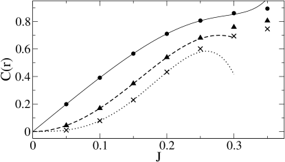
Figure 3: Atom-atom correlations as a function of the tunneling $J$. Numerics for $M=40$ system: $C(1)$ (dots), $C(2)$ (triangles), $C(3)$ (x’s). Lines: solid, dashed, dotted represent perturbative expansions (III) of $C(1)$, $C(2)$, $C(3)$, respectively.

Finally we discuss the density-density correlations. They can be determined in a counting experiment almost the same as the one discussed for ${\rm Var}(\hat{n})$ measurement, except for the fact that now atoms from two depleted sites have to be counted first. A perturbation theory predicts (LABEL:D) with accuracy of ${\cal O}(J^{16})$. This data and our results for $D(4\cdots 7)$ reveal that $D(r>0)=1-{\cal O}(J^{2r})$.

The comparison between the expansion and the numerics is presented in Fig. 4: there is a good agreement up to $J$ equal to $0.2\sim 0.225$, which may be a little surprising concerning high order of (LABEL:D). One may attribute it to presence of open boundary conditions introducing small inhomogeneities in atoms density in our numerics. On the other hand, the effects of open boundaries will always be present in an experimental setup proposed in raizen . Thus, our numerical calculations might actually better represent the experimental situation than the expansion (LABEL:D) derived for an idealized infinite lattice.

Our perturbative predictions can be tested for self-consistency, e.g., the following identity can be derived from the eigenequation for the ground state energy:

$${\cal E}=-2JC(1)+\frac{{\rm Var}(\hat{n})^{2}}{2}.$$

Using (3), (4) and (III) one easily shows that indeed it exactly holds up to ${\cal O}(J^{16})$ terms, as expected from the orders of expansions presented in this paper.

Though it is known that mean-field theory works badly in 1D, it is instructive at this point to compare our findings to predictions of the most popular mean-field, i.e., a Gutzwiller variational wave function jaksch ; krauth . This approach predicts in 1D, at unit filling factor, that the ground state is $|1,1,\dots\rangle$ for $0\leq J\leq 1/11.6$, which is interpreted as a MI phase. It implies that in this $J$ range: ${\cal E}=0$, ${\rm Var}(\hat{n})=0$, $C(r)=0$, $D(r)=1$. Our results analytically quantify the amount of discrepancy between these mean-field predictions and the exact ones. It would be also instructive to compare our findings to predictions of the perturbatively improved Gutzwiller approach schroll .

$$D(1) = 1-4J^{2}+\frac{136}{3}J^{4}-\frac{2008}{27}J^{6}-\frac{150638}{81}J^{8}+\frac{4897282}{729}J^{10}-\frac{415922848153}{14696640}J^{12}+\frac{1022120948444278027}{7777461888000}J^{14},$$

$$D(2) = 1-\frac{100}{3}J^{4}+\frac{2128}{3}J^{6}-\frac{1156462}{243}J^{8}-\frac{6848011}{729}J^{10}+\frac{10808763042127}{44089920}J^{12}-\frac{5150051155340205251}{3888730944000}J^{14},$$

$$D(3) = 1-\frac{13064}{27}J^{6}+\frac{3727066}{243}J^{8}-\frac{1588041877}{8748}J^{10}+\frac{1710030328933}{2755620}J^{12}+\frac{2208787916976404357}{370355328000}J^{14}.$$

IV Symmetry of perturbative expansions

Expansions of ${\cal E}$, $C(r)$, and $D(r)$ have well defined parity with respect to the $J\to-J$ transformation. That is explained below, and provides an insight into the $J\to-J$ symmetry of the BHM. Additionally, it helps in determining the accuracy of our perturbative predictions. Indeed, the symmetry of perturbative expansions proven below implies that if the last calculated nonvanishing term shows up in the $r$-th order, the expansion term in the $r+1$ order vanishes.

First, the ground state energy per site, Eq. (3), satisfies ${\cal E}(J)={\cal E}(-J)$. To see it one performs the canonical transformation

$$\hat{a}_{i}\to(-1)^{i}\hat{a}_{i},$$ (7)

which is a bosonic equivalent of the Shiba transformation used to prove a similar symmetry property of the Fermi-Hubbard model: Sec. 2.2.4 of FH . After the transformation, Hamiltonian (1) reads

$$\hat{H}=J\sum_{i=1}^{M}(\hat{a}_{i+1}^{\dagger}\hat{a}_{i}+{\rm h.c.})+\frac{U}{2}\sum_{i=1}^{M}\hat{n}_{i}(\hat{n}_{i}-1),$$

iff (i) the system is infinite; (ii) the system consists of even number of sites and periodic boundary conditions are applied; (iii) open boundary conditions are chosen. To the end of this paper we assume that one of these conditions holds, and that there exists a unique ground state. The transformed Hamiltonian is a $J\to-J$ version of (1), so we get the desired prediction about the symmetry of ${\cal E}(J)$.

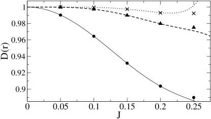
Figure 4: Density-density correlations as a function of the tunneling $J$. Numerics for $M=40$ system: $D(1)$ (dots), $D(2)$ (triangles), $D(3)$ (x’s). Perturbative expansions (LABEL:D): solid, dashed and dotted lines represent $D(1)$, $D(2)$, $D(3)$, respectively.

Second, we focus on $C(r)|_{J>0}=\langle+|\hat{a}_{j}^{\dagger}\hat{a}_{j+r}|+\rangle$, where

$$|+\rangle=\sum_{\{n_{i}\}}C_{\{n_{i}\}}(\hat{a}_{1}^{\dagger})^{n_{1}}\cdots(\hat{a}_{M}^{\dagger})^{n_{M}}|{\rm vac}\rangle$$ (8)

is a ground state of (1) with $J>0$ [$C_{\{n_{i}\}}$ are some coefficients and $\hat{a}_{i}|{\rm vac}\rangle=0$]. Using (7), one gets that the ground state of the Hamiltonian (1) with $J<0$ is (up to a phase factor):

$$|-\rangle=\sum_{\{n_{i}\}}(-1)^{\sum jn_{j}}C_{\{n_{i}\}}(\hat{a}_{1}^{\dagger})^{n_{1}}\cdots(\hat{a}_{M}^{\dagger})^{n_{M}}|{\rm vac}\rangle,$$

where $C_{\{n_{i}\}}$ are the same as in (8). An explicit calculation shows that $C(r)|_{J<0}=\langle-|\hat{a}_{j}^{\dagger}\hat{a}_{j+r}|-\rangle=(-1)^{r}C(r)|_{J>0}$, therefore $C(r)\to(-1)^{r}C(r)$ as $J\to-J$: see (5) for an example when $\sum n_{i}=M\to\infty$.

Third, following above calculation, one shows that $D(r)$ and ${\rm Var}(\hat{n})$ does not change under $J$ sign inversion. The latter result is shadowed by explicit assumption of $J>0$ during Taylor expansion leading to (4).

Finally, we note that the ground state of two component Bose-Einstein condensate in an optical lattice was found to change after inversion of $J$ sign graham . Our paper provides tools for a closer inspection of this interesting finding.

V Summary

In this paper, we have derived and discussed analytical predictions on important quantities describing physics of the Mott phase: variance of on-site number operator, atom-atom and density-density correlation functions. We have also explored, for the first time to our knowledge, the fundamental $J\to-J$ symmetry of the BHM. We expect that our findings can be useful in interpretation of ongoing experiments performed in homogeneous lattices filled with ultracold atoms.

We would like to acknowledge insightful discussions with Dominique Delande, Mark Raizen, and Eddy Timmermans, as well as the financial support from the US Department of Energy. Calculations based on Vidal’s algorithm were done in ICM UW under grant G29-10. J.Z. was supported by Polish Government scientific funds (2005-2008).

Appendix A Perturbative expansion

Here we sketch some of technical details of the nondegenerate perturbative expansions that we perform.

To introduce the notation: the Hamiltonian (1) is re-written as $\hat{H}_{0}+\lambda\hat{V}$, where $\lambda=-J$, $\hat{H}_{0}=\frac{1}{2}\sum_{i=1}^{M}\hat{n}_{i}(\hat{n}_{i}-1)$, $\hat{V}=\sum_{i=1}^{M}(\hat{a}_{i+1}^{\dagger}\hat{a}_{i}+{\rm h.c.})$.

The ground state wave-function and eigenenergy up to a given order are

$$|\Psi\rangle=\sum_{r=0}^{S}\lambda^{r}|\varphi(r)\rangle,\ \ E=\sum_{r=0}^{S+1}\lambda^{r}{\cal E}_{r},$$ (9)

$$|\varphi(r)\rangle=\sum_{i}a^{(r)}_{i}|i\rangle,\ \ \hat{H}_{0}|i\rangle=e_{i}|i\rangle,\ \ \langle i|j\rangle=\delta_{ij}.$$ (10)

To keep the wave function (9) normalized to unity we must satisfy $\langle\Psi|\Psi\rangle=1+{\cal O}(\lambda^{S+1})$. It implies that $\langle\varphi(0)|\varphi(0)\rangle=1$ and granice

$$\langle\varphi(0)|\varphi(r)\rangle=-\frac{1}{2}\sum_{i=1}^{r-1}\langle\varphi(i)|\varphi(r-i)\rangle,\ \ r=1,\dots,S.$$ (11)

The wave function (9) follows the eigen-equation

$$(\hat{H}_{0}+\lambda\hat{V})|\Psi\rangle=E|\Psi\rangle,$$ (12)

which in the $\lambda^{0}$ order implies that $|\varphi(0)\rangle=a_{0}^{(0)}|0\rangle=|0\rangle$ (after proper choice of basis), and ${\cal E}_{0}=e_{0}$. In higher orders $a_{0}^{(r)}=\langle 0|\varphi(r)\rangle$ is found from (11).

The coefficients $a^{(r\geq 1)}_{i\neq 0}$ (10) are obtained from projection of (12) onto basis states $\{|i\neq 0\rangle\}$ (10)

$$a^{(r)}_{i}(e_{i}-e_{0})+\sum_{j}\langle i|\hat{V}|j\rangle a^{(r-1)}_{j}=\sum_{k=1}^{r-1}{\cal E}_{k}a^{(r-k)}_{i}.$$ (13)

The eigenenergies are found from a projection of (12) onto $|0\rangle$ granice

$${\cal E}_{r}=\sum_{j}\langle 0|\hat{V}|j\rangle a^{(r-1)}_{j}-\sum_{k=1}^{r-1}{\cal E}_{k}a^{(r-k)}_{0},$$ (14)

where $r=1,\dots,S+1$. Equations (11), (13) and (14) have to be solved order by order starting from $r=1$.

In our calculations

$$|\varphi(0)\rangle:=|0\rangle=|1,1,\dots\rangle,$$ (15)

and

$$|i\rangle=|n_{1i},n_{2i},\dots,n_{Mi}\rangle,\ \ e_{i}=\frac{1}{2}\sum_{k}(n_{ki}-1)n_{ki}.$$ (16)

Efficient manipulations on Fock states (16) are crucial for getting high order expansions on a computer. We have achieved it by using a fast mapping $\{n_{1i},n_{2i},\dots,n_{Mi}\}\to i$ which was provided by the hash functions – see knuth for their general description.

Since $e_{i}$ (16) is an integer number and the action of $\hat{V}$ onto a Fock state produces factors of the form $\sqrt{n_{k\pm 1}+1}\sqrt{n_{k}}$ ($n_{k}$ is the atom occupation of the k-th lattice site), we see from (13) and (14) that every $a_{i}^{(r)}$ coefficient will be in general equal to

$$a^{(r)}_{i}=\sum_{s=1}^{s_{\rm max}}\frac{b\left(\{r,i\},s\right)}{c\left(\{r,i\},s\right)}\sqrt{\prod_{k=1}^{k_{\rm max}}p\left(\{r,i\},s,k\right)},$$ (17)

where $b(\{r,i\},s)$ and $c(\{r,i\},s)$ are integer numbers and $p(\{r,i\},s,k)$ are prime numbers satisfying $p(\{r,i\},s,k)\leq r+1$ – notice that when we develop the expansion around the Fock state (15) the highest on-site occupation in the $r$-th order is $r+1$ because it originates from $r$ consecutive actions of $\hat{V}$ operator onto (15). Similarly, one finds that $k_{\rm max}(\{r,i\},s)\leq r$.

We have done the symbolic calculations by writing a proper ${\cal C}$ code. Each set of $\{p(\{r,i\},s,k):k=1\dots k_{\rm max}\}$ has been encoded in bits of a single integer number, while every $b(\{r,i\},s)/c(\{r,i\},s)$ ratio has been allocated as a Gnu Multi Precision rational number gmp . The first choice minimizes the memory requirements on storage of the prime number part, while the latter one allows for avoiding overflows occurring at high order expansions when $b(\{r,i\},s)$ and $c(\{r,i\},s)$ are allocated as integer numbers. To reduce usage of memory the $s_{\rm max}$ parameter has to be set as small as possible during allocation process. By running the program we found that $s_{\rm max}=2$ is sufficient for all the calculations performed in this paper.

The results of the symbolic calculations were directly verified by calculation of the perturbative expansion in a numeric (as opposed to a symbolic) way. There we treat $a^{(r)}_{i}$ as double precision numbers avoiding complications of symbolic manipulations. Results obtained numerically are in agreement with the symbolic ones within accuracy provided by the double precision format.

Appendix B Noninteracting system

It is instructive to briefly summarize here the predictions for various observables in the limit of negligible atom interactions, say $U\equiv 0$ case.

The $N$- particle ground state of the non-interacting $M$- site Hubbard model (1) with periodic boundary conditions is given by

$$|SF\rangle=\frac{1}{\sqrt{N!M^{N}}}\left(\sum_{i=1}^{M}\hat{a}_{i}^{\dagger}\right)^{N}|{\rm vac}\rangle,$$ (18)

where $\hat{a}_{i}|{\rm vac}\rangle=0$ and $\langle SF|SF\rangle=1$ – notice that (18) is nothing else than the $N$- particle zero momentum ground state stoof . The ground state eigenenergy equals $-2JN$.

After some algebra (18) can be rewritten to the form

$$|SF\rangle=\sqrt{\frac{N!}{M^{N}}}\sum_{\{n_{i}\}}\frac{|n_{1},\dots,n_{M}\rangle}{\sqrt{n_{1}!\cdots n_{M}!}},$$ (19)

where the sum goes over all sets of boson on-site occupation (integer) numbers $\{n_{i}\}$ such that $\sum_{i}n_{i}=N$ and $0\leq n_{i}\leq N$. The wave-function (19) allows for an easy calculation of different expectation values. Indeed, the summation can be expressed as $\sum_{\{n_{i}\}}=\sum_{n_{1}=0}^{N}\cdots\sum_{n_{M}=0}^{N}\delta_{n_{1}+\cdots+n_{M},N}$, then the Kronecker delta can be represented as $\delta_{l,m}=\frac{1}{2\pi}\int_{0}^{2\pi}d\varphi[\exp(i\varphi)]^{l-m}$, and finally the integration over $\varphi$ can be replaced by the integration over $z=\exp(i\varphi)$ on the unit circle surrounding the origin of the complex $z$ plane. Usage of the residue theorem allows for getting that

$${\rm Var}(\hat{n})=\sqrt{\frac{N}{M}-\frac{N}{M^{2}}},\ \ C(r)=\frac{N}{M},\ \ D(r)=\frac{N(N-1)}{M^{2}},$$

for any integer $N>0$ and $M<r$.

In this paper we are interested in the case of $N/M=1$ and $M\gg 1$, i.e.,

$${\rm Var}(\hat{n})=1,\ \ C(r)=1,\ \ D(r)=1.$$ (20)

References

- (1) D. Jaksch, C. Bruder, J.I. Cirac, C.W. Gardiner, and P. Zoller, Phys. Rev. Lett. 81, 3108 (1998).
- (2) M. Greiner, O. Mandel, T. Esslinger, T.W. Hänsch, and I. Bloch, Nature 415, 39 (2002).
- (3) T. Stöferle, H. Moritz, C. Schori, M. Köhl, and T. Esslinger, Phys. Rev. Lett. 92, 130403 (2004).
- (4) D. Jaksch and P. Zoller, Ann. Phys. (N.Y.) 315, 52 (2005).
- (5) W. Hofstetter, J.I. Cirac, P. Zoller, E. Demler, and M.D. Lukin, Phys. Rev. Lett. 89, 220407 (2002).
- (6) A. Sanpera, A. Kantian, L. Sanchez-Palencia, J. Zakrzewski, and M. Lewenstein, Phys. Rev. Lett. 93, 040401 (2004).
- (7) L.M. Duan, E. Demler, and M.D. Lukin, Phys. Rev. Lett. 91, 090402 (2003).
- (8) B. Damski, H.-U. Everts, A. Honecker, H. Fehrmann, L. Santos, and M. Lewenstein, Phys. Rev. Lett. 95, 060403 (2005).
- (9) M.P.A. Fisher, P.B. Weichman, G. Grinstein, and D.S. Fisher, Phys. Rev. B 40, 546 (1989).
- (10) S. Sachdev, Quantum Phase Transitions (Cambridge University Press, Cambridge UK, 2001).
- (11) D. Jaksch, H.-J. Briegel, J.I. Cirac, C.W. Gardiner, and P. Zoller, Phys. Rev. Lett. 82, 1975 (1999); G.K. Brennen, C.M. Caves, P.S. Jessen, and I.H. Deutsch, Phys. Rev. Lett. 82, 1060 (1999).
- (12) G.G. Batrouni, R.T. Scalettar, and G.T. Zimanyi, Phys. Rev. Lett. 65, 1765 (1990).
- (13) W. Krauth, M. Caffarel, and J.-P. Bouchaud, Phys. Rev. B 45, 3137 (1992).
- (14) T.D. Kühner and H. Monien, Phys. Rev. B 58, R14741 (1998); R.V. Pai, R. Pandit, H.R. Krishnamurthy, and S. Ramasesha, Phys. Rev. Lett. 76, 2937 (1996).
- (15) N. Elstner and H. Monien, Phys. Rev. B 59, 12184 (1999); cond-mat/9905367 (unpublished).
- (16) T.D. Kühner, S.R. White, and H. Monien, Phys. Rev. B 61, 12474 (2000).
- (17) G.G. Batrouni et al., Phys. Rev. Lett. 89, 117203 (2002); G.G. Batrouni, F.F. Assaad, R.T. Scalettar, and P.J.H. Denteneer, Phys. Rev. A 72, 031601(R) (2005); P. Sengupta, M. Rigol, G.G. Batrouni, P.J.H. Denteneer, and R.T. Scalettar, Phys. Rev. Lett. 95, 220402 (2005).
- (18) T.P. Meyrath, F. Schreck, J.L. Hanssen, C.-S. Chuu and M.G. Raizen, Phys. Rev. A 71, 041604(R) (2005); M.G. Raizen, private communication.
- (19) L. Amico, A. Osterloh, and F. Cataliotti, Phys. Rev. Lett. 95, 063201 (2005).
- (20) G. Vidal, Phys. Rev. Lett. 93, 040502 (2004).
- (21) A.J. Daley et al., J. Stat. Mech.: Theor. Exp. P04005 (2004).
- (22) M.P. Gelfand, R.R.P. Singh, and D.A. Huse, J. Stat. Phys. 59, 1093 (1990).
- (23) A. Honecker, Phys. Rev. B 59, 6790 (1999); C. Knetter, K.P. Schmidt, and G.S. Uhrig, Eur. Phys. J. B 36, 525 (2003).
- (24) E. Brézin, J.C. Le Guillou, and J. Zinn-Justin, Phys. Rev. D 15, 1544 (1977).
- (25) V.A. Kashurnikov, N.V. Prokof’ev, and B.V. Svistunov, Phys. Rev. A 66, 031601(R) (2002).
- (26) C. Schroll, F. Marquardt, and C. Bruder, Phys. Rev. A 70, 053609 (2004).
- (27) F.H.L. Essler, H. Frahm, F. Göhmann, A. Klümper, and V.E. Korepin, The one dimensional Hubbard model (Cambridge University Press, Cambridge UK, 2005).
- (28) K.V. Krutitsky and R. Graham, Phys. Rev. Lett. 91, 240406 (2003).
- (29) If the upper summation limit is smaller then the lower one, the sum equals zero by definition.
- (30) D.E. Knuth, The art of computer programming (Addison-Wesley, Boston USA, 1998) – see volume 3 in the second edition.
- (31) www.swox.com/gmp.
- (32) D. van Oosten, P. van der Straten, and H.T.C. Stoof, Phys. Rev. A 63, 053601 (2001).