From stripe to checkerboard order on the square lattice
in the presence of quenched disorder

Abstract

We discuss the effects of quenched disorder on a model of charge density wave (CDW) ordering on the square lattice. Our model may be applicable to the cuprate superconductors, where a random electrostatic potential exists in the CuO₂ planes as a result of the presence of charged dopants. We argue that the presence of a random potential can affect the unidirectionality of the CDW order, characterized by an Ising order parameter. Coupling to a unidirectional CDW, the random potential can lead to the formation of domains with 90 degree relative orientation, thus tending to restore the rotational symmetry of the underlying lattice. We find that the correlation length of the Ising order can be significantly larger than the CDW correlation length. For a checkerboard CDW on the other hand, disorder generates spatial anisotropies on short length scales and thus some degree of unidirectionality. We quantify these disorder effects and suggest new techniques for analyzing the local density of states (LDOS) data measured in scanning tunneling microscopy experiments.

I Introduction

One of the major stumbling blocks preventing a quantitative confrontation between theory and experiment in the cuprate superconductors is the influence of quenched disorder on the experimental observations. The dopant ions exert a significant electrostatic potential on the CuO₂ plane, and so unless the ions can be carefully arranged in a regular pattern, the mobile charge carriers experience a random potential. Recent STM observation hanaguri ; fang ; ali ; mcelroy ; hashimoto clearly display that quenched randomness is crucial in determining the spatial modulations of the local density of states.

There has been much recent interest in determining the nature of the spin and charge density wave order (CDW) observed in STM, neutron, and X-ray scattering in a variety of cuprate compounds at low temperatures hanaguri ; fang ; ali ; mcelroy ; hashimoto ; Tranquada+97 ; Lee+99 ; tranquada+04 ; abbamonte . The quenched disorder acts on the CDW order as a “random field”, which is always a relevant perturbation at low temperatures: true long-range order is disrupted at any finite random field strength apy . Nevertheless, one might hope that an analytic treatment may be possible in the limit of weak random fields. Many such analysesapy ; natter90 ; giam ; dsf ; nattermann have been carried out in the literature, describing states with power-law correlations and suppressed dislocations (or related topological defects) at intermediate length scales. At the longest scales, dislocations always proliferate and all correlations are expected to decay exponentially; no analytic treatment is possible in this strong coupling regime. As we will discuss below, current experiments on the cuprates are in a regime dominated by dislocations, and there does not appear to be any significant regime of applicability of the defect-free theory. Consequently, we are forced to rely on numerical simulations for an understanding of experiments. We will present numerical results over a representative range of parameters. Our aim is to allow insights into the underlying theory by a comparison of experimental and numerical results.

II Model

A previous work by two of the authors delmaestro studied the influence of thermal fluctuations on density wave order on the square lattice. Here, we will study the influence of quenched randomness on the same underlying theory. A generic density was defined which could be any observable invariant under spin rotations and time reversal

$$\delta\rho(\boldsymbol{r})=\mbox{Re}\left[\Phi_{x}\mathrm{e}^{i\boldsymbol{K}_{x}\cdot\boldsymbol{r}}\right]+\mbox{Re}\left[\Phi_{y}\mathrm{e}^{i\boldsymbol{K}_{y}\cdot\boldsymbol{r}}\right],$$ (1)

where ${\bf K}_{x}=(2\pi/a)(1/p,0)$, ${\bf K}_{y}=(2\pi/a)(0,1/p)$, and $\Phi_{x,y}$ are complex order parameters which were assumed to vary slowly on the scale of a lattice spacing.

If both amplitudes $|\Phi_{x,y}|$ have nonzero expectation values, the charge density is modulated in both $x$- and $y$-directions and describes a solid on the square lattice. In addition, if the wave length of the charge ordering is commensurate with the underlying crystal, i.e. for integer $p$, the density displays true long range order. For incommensurate charge order, fluctuations due to finite temperature will cause quasilong–range order with a power law decay of correlation functions. If only one of the two amplitudes $|\Phi_{x,y}|$ has nonzero expectation value, the density Eq. (1) describes unidirectional (striped) CDW order. Again, the presence of a commensurate lattice potential makes the order long ranged at finite temperatures, whereas in the incommensurate case it is quasilong–ranged.

In the incommensurate phase, in the absence of disorder, the most general free energy density expanded in powers of $\Phi_{x,y}$ and its gradients consistent with the symmetries of the square lattice is given by

$$\mathcal{F}_{\Phi} = \int d^{2}r\Bigl{[}C_{1}\left(\left|\partial_{x}\Phi_{x}\right|^{2}+\left|\partial_{y}\Phi_{y}\right|^{2}\right)$$ (2)

$$+\ C_{2}\left(\left|\partial_{y}\Phi_{x}\right|^{2}+\left|\partial_{x}\Phi_{y}\right|^{2}\right)+\ C_{3}\left|\partial_{x}\Phi_{x}\right|\left|\partial_{y}\Phi_{y}\right|$$

$$~{}~{}~{}~{}~{}~{}+\ s\left(|\Phi_{x}|^{2}+|\Phi_{y}|^{2}\right)+\frac{u}{2}\left(|\Phi_{x}|^{2}+|\Phi_{y}|^{2}\right)^{2}$$

$$~{}~{}~{}~{}~{}~{}+\ v|\Phi_{x}|^{2}|\Phi_{y}|^{2}\Bigr{]}.$$

The homogeneous mean field solution of this model is summarized in Fig. 1 where the checkerboard, stripe and liquid phase values of $\Phi_{x,y}$ are shown along with the accompanying free energy densities.

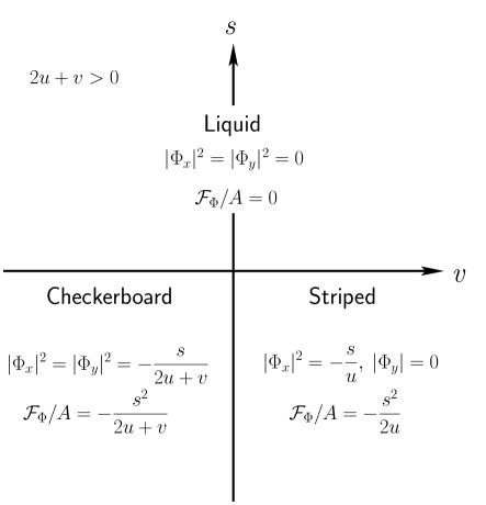
Figure 1: The homogeneous mean field solutions of Eq. (2) for $\Phi_{x,y}$.

In this work we focus on the influence of quenched disorder on CDW order and thus consider adding a term to the free energy consisting of two complex random fields, coupling directly to $\Phi_{x,y}$

$$\mathcal{F}_{\mathrm{H}}=-\int d^{2}r\left(\mathrm{H}_{x}^{*}\Phi_{x}+\mathrm{H}_{y}^{*}\Phi_{y}+c.c.\right)$$ (3)

resulting in the total action

$$\mathcal{F}=\mathcal{F}_{\Phi}+\mathcal{F}_{\mathrm{H}}$$ (4)

where the complex random fields $\mathrm{H}_{\mu}$ ($\mu=x,y$) are parameterized as $\mathrm{H}_{\mu}(\boldsymbol{r})=h_{\mu}(\boldsymbol{r})\mathrm{e}^{i\eta_{\mu}(\boldsymbol{r})}$, $h_{\mu}$ are Gaussian distributed random variables with mean $0$, and standard deviation $h_{0}$ and $\eta_{\mu}$ are uniformly distributed random phases on $[0,2\pi)$.

Let us confine ourselves to the condensed phase where $s<0$, and $u>0$ for stability. The interesting physics are encapsulated by the effects of altering the coupling constant $v$ and the variance of the random field $h_{0}$. While $v$ changes the low energy ground states from checkerboard like configurations for $v<0$ ($|\Phi_{x}|=|\Phi_{y}|$) to stripe like patterns ($|\Phi_{\mu}|\neq|\Phi_{\nu}|=0$) for $v>0$, the variance $h_{0}$ should destabilize both types of states.

A careful treatment of the coupling between CDW order and a random electrostatic potential yields random compression terms of the form nattermann $\mathrm{h}_{\mu}\partial\Theta_{\mu}$ ($\Theta_{\mu}=\mathrm{arg}[\Phi_{\mu}]$) omitted in the free energy Eq. (3). In addition, an RG analysis of the full action $\mathcal{F}_{\Phi}+\mathcal{F}_{\mathrm{H}}$ generates random shear terms. Random compression and shear terms are responsible for the power law decay of correlation functions on intermediate length scales, on which the influence of topological excitations (dislocations) in the phase fields $\Theta_{\mu}$ can be neglectednattermann .

In STM experiments, the correlation length of charge order is found to have values ranging fromhanaguri 2.5, to roughlyali 5 CDW periods. In neutron scattering experiments, peak widths corresponding to correlation lengths larger then ten CDW periods were observed Tranquada+97 ; Lee+99 . The correlation length describes the scale on which dislocations proliferate, and the presence of a relatively short correlation length indicates that there is no intermediate length scale on which compression and shear terms are important. For this reason, the omission of these terms from the elastic energy should be justified.

III Numerical Minimization

Due to the presence of the two complex random fields $\mathrm{H}_{\mu}(\boldsymbol{r})$, we have elected to minimize Eq. (4) numerically. The interplay of elastic and disorder energy causes frustration and gives rise to an exponentially large number of low lying states with similar energies but very different configurations. As these states are separated by large energy barriers, relaxation after an external perturbation is very slow and glassy dynamics can be observed. For these reasons, numerically finding the ground state of such a system is a hard problem and as novel algorithms are developed and employed, even to relatively simple models, new states with lower energies are inevitably found weigel .

Gradient methods which move strictly downhill in the energy landscape are fast, but prone to becoming stuck in local minima and are not always able to reproduce the results of slower ergodic methods. Simulated annealing algorithms KiGeWe83 have been the most successful at thoroughly sampling the possible configuration space by using a fictitious temperature. By successively lowering this temperature, the resolution of finer and finer energy scales becomes possible while avoiding the danger of being stuck in a metastable excited state.

As a compromise we have elected to employ a combination of both greedy conjugate gradient shewchuk and ergodic simulated annealing siarry methods. We allow for the possibility of local uphill moves where the configuration update involves making a downhill step in a random area of the sample. The size of the randomly chosen region is annealed by tracking metropolis acceptance rate. This method faithfully reproduces quite quickly, the results of early Monte Carlo work on the random field XY model gingras .

We have performed simulations for a number of lattice sizes $L=\{20,32,48,64,100\}$, commensurate with the experimentally observed hanaguri ; ali ; fang ; mcelroy period of modulations in the local density of states of four lattice spacings ($p=4$) and multiple realizations of disorder $N_{rd}(L)=\{200,200,150,150,100\}$.

Let us consider a $L\times L$ square lattice of $N$ sites labelled by $i$, then after rescaling to give dimensionless coupling parameters the continuum action Eq. (4) in units where the lattice constant $a_{0}$ is set to unity and $C_{3}=0$ takes the form (with $\Theta_{\mu,{i}}=\mathrm{arg}[\Phi_{\mu,i}]$)

$$\mathcal{F}_{L} = -\frac{1}{2}\sum_{\mu=x,y}\sum_{\langle i,j\rangle}J_{\mu,j}|\Phi_{\mu,{i}}||\Phi_{\mu,{j}}|\cos(\Theta_{\mu,{i}}-\Theta_{\mu,{j}})$$ (5)

$$+\ \sum_{\mu=x,y}\sum_{i}\Bigl{[}(C_{1}+C_{2}+s)|\Phi_{\mu,{i}}|^{2}+\frac{u}{2}|\Phi_{\mu,{i}}|^{4}$$

$$-\ 2h_{\mu,i}|\Phi_{\mu,{i}}|\cos(\Theta_{\mu,{i}}-\eta_{\mu,{i}})\Bigr{]}$$

$$+\ (u+v)\sum_{i}|\Phi_{x,i}|^{2}|\Phi_{y,i}|^{2}$$

with $\langle i,j\rangle$ indicating the usual sum over nearest neighbors and the factor of $1/2$ is inserted to avoid double counting. The coupling matrix $J_{\mu,j}$ has diagonal elements $J_{x,i\pm x}=J_{y,i\pm y}=C_{1}$ and off diagonal couplings $J_{x,i\pm y}=J_{y,i\pm x}=C_{2}$. We have chosen to set $C_{1}=C_{2}=1$ and $s=-0.1$ thus restoring full rotational symmetry of the elastic energy on scales much larger than the lattice spacing and confining our analysis to the condensed phase. We have also elected to pick the value of the quartic coupling $u$ to ensure the condensation energy remains constant across the critical line $v=0$ by setting $u(v\geq 0)=-s$ and $u(v<0)=-(s+v/2)$.

IV Results

Employing this minimization procedure we obtain stable low energy field configurations like the ones shown in Figs. 2 to 4.

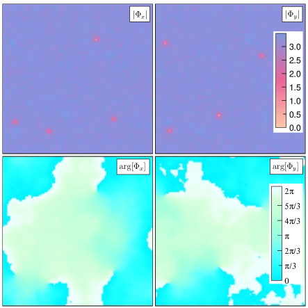
Figure 2: The ground state field configuration on a $100\times 100$ lattice for a random field standard deviation of $h_{0}=0.6$ and $xy$-interaction $v=-0.1$ for a particular realization of disorder.

For $v=-0.1$ and $h_{0}=0.6$ (Fig. 2) we observe small circular regions less then 5 lattice spacings across, where the local random field configuration has taken a value that makes it energetically favorable to suppress the magnitude of either $\Phi_{x}$ or $\Phi_{y}$ in its vicinity.

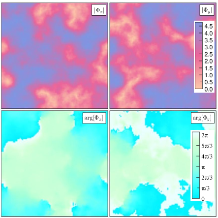
Figure 3: The ground state field configuration on a $100\times 100$ lattice for a random field standard deviation of $h_{0}=0.6$ and $xy$-interaction $v=0.0$ for a particular realization of disorder.

For the uncoupled theory (Fig. 3) $\Phi_{x,y}$ appear much smoother and although there still exists separate regions of stripe and checkerboard order, the interfaces between these regions are poorly defined.

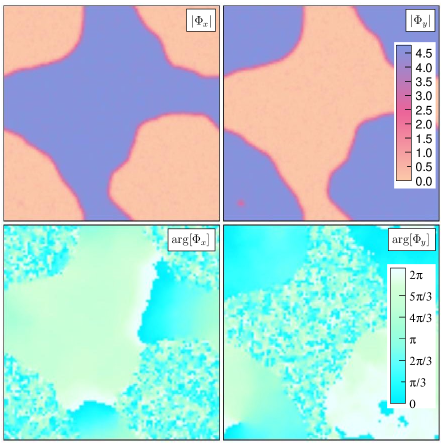
Figure 4: The ground state field configuration on a $100\times 100$ lattice for a random field standard deviation of $h_{0}=0.6$ and $xy$-interaction $v=0.1$ for a particular realization of disorder. The phase of $\Phi_{x,y}$ fluctuates strongly in regions where its amplitude is suppressed.

We may also observe the effects of positive $v=0.1$ at the same disorder strength as seen in Fig. 4. In this case, the magnitude of either $\Phi_{x}$ or $\Phi_{y}$ is suppressed to zero over large regions of the sample leading to a ground state field configuration with well defined domains having unidirectional order in either the $x$- or $y$-directions.

We can construct the form of the density fluctuations $\delta\rho(\boldsymbol{r})$ (Eq. (1)) from the minimized value of the spatially dependent order parameters to determine the effects of altering $v$ and $h_{0}$ as seen in Fig. 5.

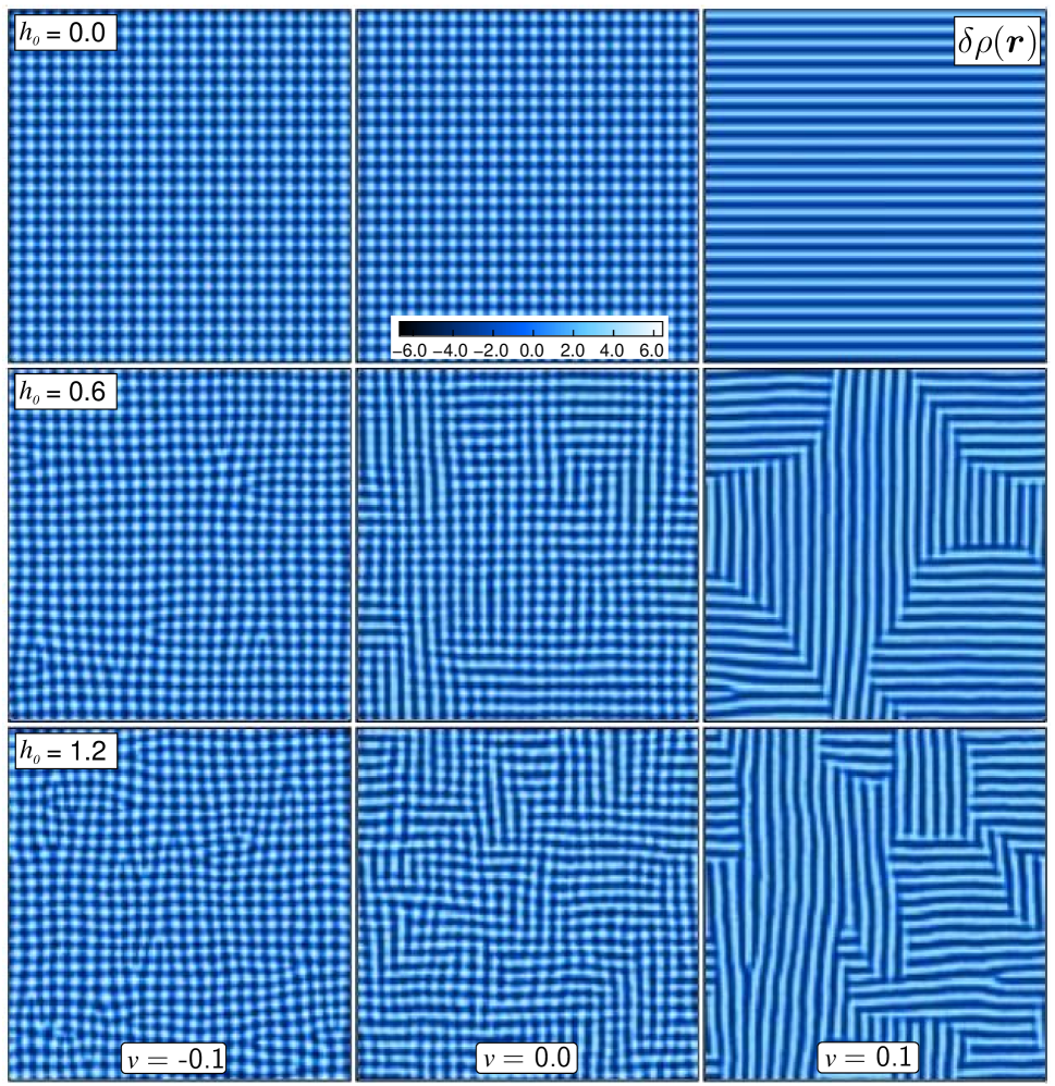
Figure 5: The density fluctuations $\delta\rho(\boldsymbol{r})$ on a $100\times 100$ lattice for $v=-0.1$ (left column), $v=0.0$ (center column) and $v=0.1$ (right column) with $h_{0}=0.0,0.6$ and $1.2$ from top to bottom for one random field configuration. The central row was constructed using the values of $\Phi_{x,y}$ from Figs. 2 through 4.

For $v<0$ and $h_{0}=0.0$ we observe robust checkerboard ordering which is coherent over the entire lattice. As the variance of the random field is increased, dislocations in the phase of the $\Phi_{\mu}$ fields gradually destroy the local ordering, and the correlation length is reduced to less than three CDW periods for $h_{0}=1.2$. For $v=0.0$ and $h_{0}=0.0$, the mean field critical value in the disorder free theory, density fluctuations in the $x$- and $y$-direction have a period of four lattice spacings and identical amplitudes. However, the response of the system to increasing $h_{0}$ is very different than in the $v=-0.1$ case. For any finite amount of disorder, there is a significant enhancement in the size of unidirectional correlations as the sample breaks up into regions with the magnitude of either $\Phi_{x}$ or $\Phi_{y}$ greatly reduced. In the clean limit with $v>0$ we obtain purely unidirectional density fluctuations. As the strength of disorder is increased, large domains of $\pi/2$ relatively orientated appear and finally for large values of $h_{0}$ the system breaks up into many such regions of varying sizes.

The presence of such strong stripeness leads to the natural definition of a local Ising-like order parameter krmp

$$\Sigma(\boldsymbol{r})=\frac{|\Phi_{x}(\boldsymbol{r})|^{2}-|\Phi_{y}(\boldsymbol{r})|^{2}}{|\Phi_{x}(\boldsymbol{r})|^{2}+|\Phi_{y}(\boldsymbol{r})|^{2}}$$ (6)

which measures the tendency of the system to have only one of either $\Phi_{x}$ or $\Phi_{y}$ nonzero over some finite area, with a value between -1 and 1.

As a result of our direct minimization procedure, we have calculated a full set of low energy field configurations for multiple system sizes and realizations of disorder with $xy$-couplings $v=\{-0.1,0.0,0.1,0.2\}$ and random field variances $h_{0}$ between $0.0$ and $2.0$. Using this information we can construct the disorder averaged correlation functions for each system size throughout the relevant parameter space. Two distinct types of correlations are of interest. The first are simple CDW correlation functions between the $\Phi_{\mu}$ fields given by

$$G_{\mu}(r)=\overline{\left\langle\Phi_{\mu}(r)\Phi^{*}_{\mu}(0)\right\rangle}$$ (7)

where $\mu\in\{x,y\}$ while the second type measures fluctuations of the Ising-like order parameter Eq. (6)

$$G_{\Sigma}(r)=\overline{\left\langle\Sigma(r)\Sigma(0)\right\rangle}$$ (8)

with $\langle\cdots\rangle$ indicating a spatial average in the ground state and the over-line denotes an average over multiple realizations of disorder $N_{rd}(L)$. As $L$ becomes large both $\langle\Phi_{\mu}(r)\rangle$ and $\langle\Sigma(r)\rangle$ tend to zero, and the connected and disconnected correlation functions are equivalent. Note that the definition of $G_{\Sigma}(r)$ distinguishes between regions with strong unidirectional order with $\pi/2$ relative orientation.

For sufficiently large variances in the magnitude of the random field, we expect that both Eqs. (7) and (8) will be characterized by exponential decays of the form

$$G_{\mu}(r) \sim \mathrm{e}^{-r/\xi_{\mu}}$$

$$G_{\Sigma}(r) \sim \mathrm{e}^{-r/\xi_{\Sigma}}$$ (9)

where $\xi_{\mu}$ and $\xi_{\Sigma}$ are their respective correlation lengths. $G_{\mu}(r)$ and $G_{\Sigma}(r)$ are shown for distances up to 40 lattice spacings for $v=-0.1,0.0$ and $0.1$ in Fig. 6.

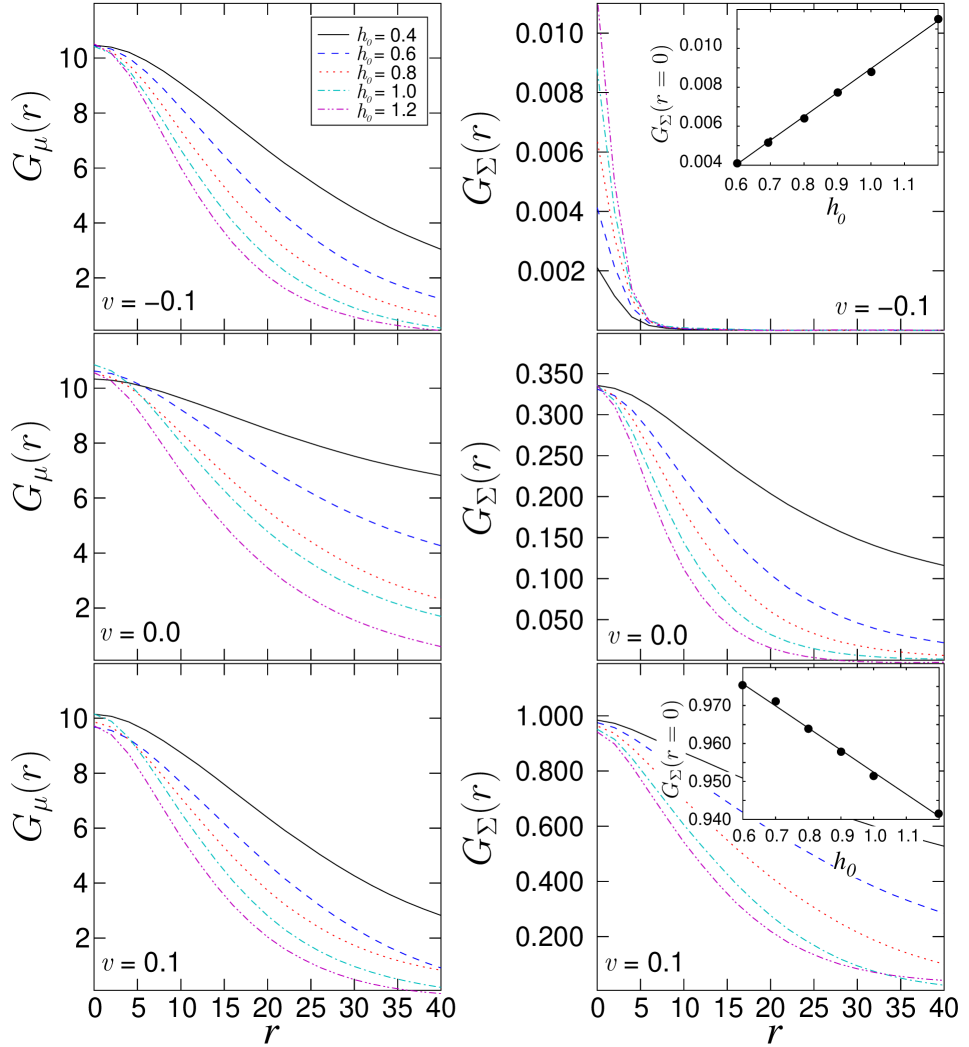
Figure 6: Selected $G_{\mu}$ and $G_{\Sigma}$ correlation functions for $v=-0.1,0.0,0.1$ and $h_{0}=0.4,0.6,0.8,1.0,1.2$ (legend applies to all panels) which were averaged over 100 realizations of disorder in a $100\times 100$ sample. The insets show $\overline{\left\langle\Sigma^{2}(0)\right\rangle}$ vs. $h_{0}$ for $v=-0.1$ (upper right) and $v=0.1$ (lower right).

All correlations appear to decay exponentially for $h_{0}\geq 0.4$, and the most striking differences between $G_{\mu}(r)$ and $G_{\Sigma}(r)$ can be seen at $r=0$ by comparing $\overline{\left\langle\Phi_{\mu}^{2}(0)\right\rangle}$ and $\overline{\left\langle\Sigma^{2}(0)\right\rangle}$. The $xy$-interaction parameter $v$ has little effect on the scale of the background CDW order, while the background Ising-like order, measured by $G_{\Sigma}(0)$, increases by three orders of magnitude as $v$ changes from $-0.1$ to $0.1$. In addition it appears that (after proper finite size scaling) $G_{\mu}(0)$ is essentially a monotonically decreasing function of $h_{0}$ from the checkerboard to stripe parameter regime. The two insets in Fig. 6 clearly show however, that the slope of $G_{\Sigma}(0)$ vs. $h_{0}$ changes from positive to negative near $v=0.0$.

In order to determine the decay constants associated with $G_{\mu}(r)$ and $G_{\Sigma}(r)$ we have performed a discrete Fourier transform of the disorder averaged correlation functions and fit them to a Lorentzian in $\boldsymbol{k}$-space for each linear system size, $xy-$interaction and random field variance. The actual correlation length is assumed to be equal to the width of the Lorentzian. Finite size scaling was then performed for each value of $v$ and $h_{0}$, as shown for $v=-0.1$ and $h_{0}=0.6$ in Fig. 7 to extract approximate infinite system size values of $\xi_{\mu}$ and $\xi_{\Sigma}$.

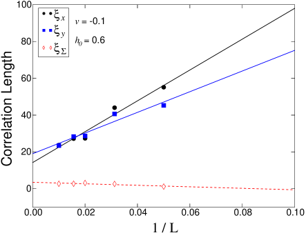
Figure 7: Finite size scaling of the correlation lengths $\xi_{x}$, $\xi_{y}$ and $\xi_{\Sigma}$ using system sizes of $L=\{20,32,48,64,100\}$ for $v=-0.1$ and $h_{0}=0.6$. $y$-intercepts were extracted to approximate $L\rightarrow\infty$.

The results of the finite size scaling procedure can be seen in Fig. 8 where we plot the decay constants associated with $G_{x}$ and $G_{\Sigma}$ as a function of random field variance $h_{0}$ for various values of $v$, the error-bars in the fits are on the order of the symbol sizes.

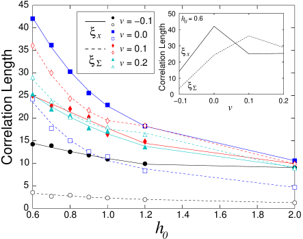
Figure 8: The correlation lengths associated with the exponential decay of $G_{x}(r)$ and $G_{\Sigma}(r)$ extracted from finite size scaled Lorentzian widths in Fourier space. Color and symbol type denote different values of $v$, closed symbols with solid lines refer to $\xi_{x}$ and open symbols with dashed lines correspond to $\xi_{\Sigma}$. The inset shows the two types of correlation lengths plotted for fixed $h_{0}$ as a function of $v$. Note that the maximum values occur at different values of the $xy$ coupling.

For a fixed value of $v$, both $\xi_{x}$ and $\xi_{\Sigma}$ decrease monotonically as a function of disorder strength. The dependence of correlation lengths on the $xy$ coupling $v$ for a fixed random field strength is more interesting, as both correlation lengths are non-monotonic functions of $v$. Changing $v$ from $-0.1$ to $0.0$, the correlation length $\xi_{x}$ increases by almost ten lattice spacings in the regime of moderate disorder strength. This increase can probably be attributed to the fact that for $v=0.0$, our model decomposes into two completely uncoupled unidirectional CDWs with ordering in the $x$ and $y$ direction, respectively. As disorder has a weaker influence on a unidirectional CDW as compared to a checkerboard CDW, this dependence of the correlation length on the value of $v$ is plausible. A further increase of $v$ to positive values leads to a reduction of $\xi_{x}$.

As $v$ controls the degree of stripe order, it is expected that the correlation length for the Ising-like order parameter increases from only a few lattice spacings for $v=-0.1$ to 20 to 40 lattice spacings for $v=0.1$ in the regime of moderate disorder strength. It is important to note that for $v=-0.1$ and $v=0.0$, Ising correlations are exclusively due to disorder fluctuations. When $v$ approaches zero coming from negative values, fluctuations of the two fields $\Phi_{x}$ and $\Phi_{y}$ are increasingly independent, and Ising correlations increase. When moving further into the stripe regime, we find $\xi_{\Sigma}(v=0.1)>\xi_{\Sigma}(v=0.2)$ for all values of $h_{0}$. This can be attributed to the sharpening of domain walls between stripey regions with relative orientation $\pi/2$ allowing them to better accommodate the value of the local random field, increasing their overall length.

While $\xi_{x}$ reaches a maximum value at $v=0$, $\xi_{\Sigma}$ peaks at $v=0.1$ (see inset of Fig. 8). The fact that these peaks occur at different values of $v$ leads to the interesting situation that $\xi_{\Sigma}>\xi_{x}$ for positive $v$. Hence, with respect to the analysis of experimental data $\xi_{\Sigma}>\xi_{x}$ is a clear signature for a striped charge order if no random potential was present. In the limit of large $v$, the system breaks up into domains with either $\Phi_{x}$ or $\Phi_{y}$ order and the correlation lengths $\xi_{x}$ and $\xi_{\Sigma}$ become equal to each other.

V Empirical Determination of Stripeness

Due to the definition of our effective model for density fluctuations on the square lattice we have the direct ability to measure the value of Eq. (6) using the ground state values of the independent CDW order parameters $\Phi_{x,y}$. However, as we wish to make contact with the STM measurements discussed in Section I it would be useful to determine a method of analyzing $\delta\rho(\boldsymbol{r})$ directly which might expose any underlying local Ising-like correlations that are not readily apparent either in real or Fourier space.

With this goal in mind, we define an effective local Ising-like order parameter $\widetilde{\Sigma}(\boldsymbol{r})$ at each point in the sample through the following procedure with more detail provided in an appendix.

1. Surround each lattice site $\boldsymbol{r}$ with a $4\times 4$ box $\Box_{\boldsymbol{r}}$ (depicted in Fig. 11) which is “centered” at the relative $(1,1)$ point.

2. Define a local density-density correlation function which lives in each $4\times 4$ box (the smallest that contains enough information to resolve the wavevectors $\{\pm\boldsymbol{K}_{x},\pm\boldsymbol{K}_{y}\}$) that is arbitrarily assigned to the $(1,1)$ point. The result is $N$ $4\times 4$ matrices

$$S_{\Box}(\boldsymbol{r},\boldsymbol{r}^{\prime}-\boldsymbol{r}^{\prime\prime})=\left\langle\delta\rho(\boldsymbol{r}^{\prime})\delta\rho(\boldsymbol{r}^{\prime\prime})\right\rangle_{\boldsymbol{r}^{\prime}-\boldsymbol{r}^{\prime\prime}\in\Box_{\boldsymbol{r}}}$$ (10)

where $\langle\cdots\rangle_{\boldsymbol{r}^{\prime}-\boldsymbol{r}^{\prime\prime}\in\Box_{\boldsymbol{r}}}$ indicates an average over all sites $\boldsymbol{r}^{\prime}\in\Box_{\boldsymbol{r}}$ and whose rows and columns are labeled by the $x$ and $y$ components of $\boldsymbol{r}^{\prime}-\boldsymbol{r}^{\prime\prime}$ employing periodic boundary conditions for the box. The specific form of one of the matrices contributing to this sum is given in Eq. (17).

3. Perform a local discrete Fourier transform of Eq. (10) using only those points in $\Box_{\boldsymbol{r}}$

$$S_{\Box}(\boldsymbol{r},\boldsymbol{k})=\frac{1}{16}\sum_{\boldsymbol{r^{\prime}}\in{\Box}_{\boldsymbol{r}}}S_{\Box}(\boldsymbol{r},\boldsymbol{r}^{\prime})\mathrm{e}^{-i\boldsymbol{k}\cdot\boldsymbol{r}^{\prime}}$$ (11)

for $\boldsymbol{k}\in\{\pm\boldsymbol{K}_{x},\pm\boldsymbol{K}_{y}\}$ at each of the $L\times L$ boxes. 4. Finally, define an effective local Ising-like order parameter as the difference of local structure factor amplitudes at $\pm\boldsymbol{K}_{x}$ and $\pm\boldsymbol{K}_{y}$ scaled by their sum in each box

$$\widetilde{\Sigma}(\boldsymbol{r})=\frac{S_{\Box}(\boldsymbol{r},\boldsymbol{K}_{x})+S_{\Box}(\boldsymbol{r},-\boldsymbol{K}_{x})-S_{\Box}(\boldsymbol{r},\boldsymbol{K}_{y})-S_{\Box}(\boldsymbol{r},-\boldsymbol{K}_{y})}{S_{\Box}(\boldsymbol{r},\boldsymbol{K}_{x})+S_{\Box}(\boldsymbol{r},-\boldsymbol{K}_{x})+S_{\Box}(\boldsymbol{r},\boldsymbol{K}_{y})+S_{\Box}(\boldsymbol{r},-\boldsymbol{K}_{y})}.$$ (12)

We may now directly compare Eqs. (6) and (12) for different values of $v$ at fixed $h_{0}$ as seen in Fig. 9.

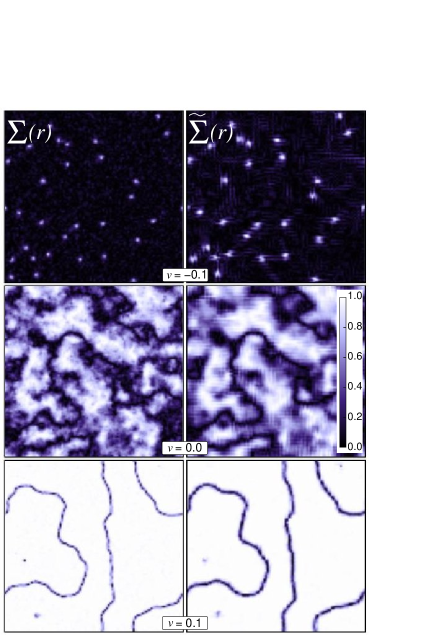
Figure 9: A comparison between the direct ($\Sigma$, left-panels) and effective ($\widetilde{\Sigma}$, right-panels) Ising-like order parameters for $h_{0}=1.0$ and $v=\{-0.1,0.0,0.1\}$ for a particular realization of disorder in a $100\times 100$ sample.

The similarity between $\Sigma(\boldsymbol{r})$ and $\widetilde{\Sigma}(\boldsymbol{r})$ is striking and shows both environs of checkerboard order (dark regions, $|\Phi_{x}(\boldsymbol{r})|=|\Phi_{y}(\boldsymbol{r})|$) and stripe order (light regions, $|\Phi_{x}(\boldsymbol{r})|\neq|\Phi_{y}(\boldsymbol{r})|=0$).

The agreement between the left and right panels in Fig. 9 can be further quantized by defining an equal point correlator

$$\mathcal{Q}=\frac{\Bigl{\langle}\Sigma(\boldsymbol{r})\widetilde{\Sigma}(\boldsymbol{r})\Bigr{\rangle}-\Bigl{\langle}\Sigma(\boldsymbol{r})\Bigr{\rangle}\Bigl{\langle}\widetilde{\Sigma}(\boldsymbol{r})\Bigr{\rangle}}{\sigma_{\Sigma}\sigma_{\widetilde{\Sigma}}}$$ (13)

where $\sigma_{\Sigma}$ is the standard deviation of $\Sigma(\boldsymbol{r})$

$$\sigma_{\Sigma}=\sqrt{\langle\Sigma^{2}(\boldsymbol{r})\rangle-\langle\Sigma(\boldsymbol{r})\rangle^{2}}.$$ (14)

Using this definition we find values for $\mathcal{Q}$ of $0.62$, $0.92$ and $0.71$ for $h_{0}=1.0$ and $v=-0.1,0.0$ and $0.1$. The smaller correlations for $v=\pm 0.1$ are due to the fact that $\Box_{\boldsymbol{r}}$ cannot be constructed symmetrically about the site $\boldsymbol{r}$ as we need to resolve the specific wavevectors $\{\pm\boldsymbol{K}_{x},\pm\boldsymbol{K}_{y}\}$ and thus small regions with rapid changes in $\Phi_{x,y}$ (sharp domain walls) will be poorly reproduced by the effective field $\widetilde{\Sigma}$.

A further comparison can be made by examining the disorder averaged values of the magnitudes of the direct and effective Ising-like order parameters,

$$\overline{|\Sigma|} = \overline{\langle|\Sigma(\boldsymbol{r})|\rangle}$$

$$\overline{|\widetilde{\Sigma}|} = \overline{\langle|\widetilde{\Sigma}(\boldsymbol{r})|\rangle}$$ (15)

which are shown in Fig. 10 for various values of $v$ as a function of disorder.

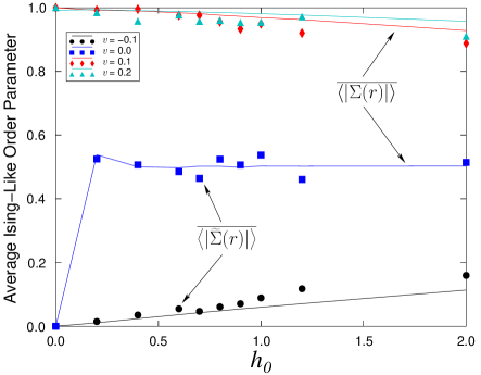
Figure 10: A comparison of the disorder averaged magnitudes of $\Sigma$ and $\widetilde{\Sigma}$ for a $100\times 100$ sample as a function of the variance of the random field. Finite size scaling appears to have little effect on these results. Symbols show the value of $\overline{\langle|\widetilde{\Sigma}(\boldsymbol{r})|\rangle}$ while lines refer to $\overline{\langle|\Sigma(\boldsymbol{r})|\rangle}$.

Again we observe significant agreement between the direct and effective Ising-Like order parameters, now having averaged over 100 realizations of disorder. At $h_{0}=0.0$ we recover the results that in the disorder free theory $\overline{|\Sigma|}$ should be identically zero for $v\leq 0$ and equal to one for $v>0$. Increasing disorder causes a smooth increase in unidirectional order for $v<0$ and a reduction for $v>0$ with the effective order parameter having a slightly larger dependence on $h_{0}$. For $v=0.0$, the magnitude of Ising-like order quickly jumps to a value near $0.5$.

The concurrence between $\Sigma(\boldsymbol{r})$ and the effective object $\widetilde{\Sigma}(\boldsymbol{r})$ inferred from the scaled difference in local structure factor peaks amplitudes at wavevectors $\pm\boldsymbol{K}_{x}$ and $\pm\boldsymbol{K}_{y}$ is not surprising in the context that they are both calculated from the same underlying complex fields $\Phi_{x,y}$ in the condensed phase. However, the utility of Eq. (12) becomes apparent when considering the plethora of experimental STM spectra where only the LDOS is measured and the underlying order is a topic of hot debate. The current analysis of such spectra involves performing a discrete Fourier transform over the entire field of view. In real materials, disorder plays an important role, and short density-density correlation lengths are often observed. Therefore, such a global Fourier transform discards a large amount of relevant local information which could in principle be used to probe any hidden electronic structure.

VI The Uncoupled Theory

In the limit of large disorder a number of results can be explained for the uncoupled theory with $v=0$.

Upon examination of the various correlation lengths in Fig. 8 it is apparent that $\xi_{x}$ is almost twice as large as $\xi_{\Sigma}$ for $v=0$. This can be understood with the help of an approximate analytical argument: for $v=0$, the lattice model Eq. (5) reduces to two uncoupled unidirectional CDWs in the $x$- and $y$-directions. Concentrating on the numerator of the Ising order parameter Eq. (6) for the moment, in the case $v=0$ the correlation function of $\Sigma$ is then proportional to $\left\langle|\Phi_{x}(r)|^{2}|\Phi_{x}(0)|^{2}\right\rangle$. If fluctuations of $\Phi_{x}$ were described by a simple Gaussian theory, this would imply $\xi_{x}=2\xi_{\Sigma}$, which indeed is approximately found in Fig. 8.

A similar approach can be used to account for the saturation of $\overline{|\Sigma|}$ and $\overline{|\widetilde{\Sigma}|}$ to $0.5$ for $v=0$ as seen in Fig. 10. Again if we assume uncoupled fluctuations in $\Phi_{x,y}$ described by a normal distribution with mean $0$ and variance $\sigma_{\Phi}^{2}$ we can directly calculate the expectation value of $\Sigma$ by performing integrals in polar coordinates

$$\left\langle\frac{(|\Phi_{x}|^{2}-|\Phi_{y}|^{2})^{2}}{(|\Phi_{x}|^{2}+|\Phi_{y}|^{2})^{2}}\right\rangle=\frac{1}{2}.$$ (16)

VII Conclusions

This paper has characterized the correlations in a disordered CDW state on the square lattice as a function of the parameter $v$ in $\mathcal{F}_{\Phi}$ (which measures the degree of unidirectionality of the CDW order, $v<0$ corresponding to checkerboard states), and the random field strength $h_{0}$. We introduced a number of diagnostics to study the nature of the disordered state: the correlation lengths, $\xi_{\mu}$, of the CDW order, the correlation length $\xi_{\Sigma}$ of the Ising order associated with the uni-directionality, the on-site amplitudes $G_{\mu}(0)$, $G_{\Sigma}(0)$, of these orders, and also discussed in Section V how closely related quantities could be measured directly in experiments.

Our results are presented in detail in Sections IV and V, and here we highlight some notable features:
(i) As is clear from the insets of Fig. 6, for $v<0$, the strength of the Ising order increases with random-field strength, while the opposite is true for $v>0$.
(ii) The correlation length $\xi_{\Sigma}>\xi_{\mu}$ only for $v>0$, and this can serve as a diagnostic for the sign of $v$ in an analysis of the experiments.
(iii) We showed that the correlator $S_{\Box}$ in Eq. (10) can serve as a very faithful diagnostic of the structure of $\Sigma$, and this should easily enable us to place experimental observations in the appropriate parameter space of the present theory.

A full interpretation of the experiments should away a direct analysis of the experimental data along the lines proposed here. Nevertheless, a comparison of the qualitative structure of the figures presented here (especially Fig 5) with e.g. the STM observations of Ca_2-xNa_xCuO₂Cl₂ by Hanaguri et al. does indicate that this system has a value of $v$ close to zero and likely positive.

For the future, our approach offers an avenue to quantitatively correlate the STM experiments with neutron scattering. In particular, after determining the appropriate parameter regime of $\mathcal{F}_{\Phi}$ from an analysis of the STM data, the resulting $\delta\rho(\boldsymbol{r})$ configurations can be used as an input to determining the dynamic spin structure factor, as discussed in recent works ssvojta ; ribhu .

While this paper was being completed, we learned of related results obtained by Robertson et al. robertson .

Appendix A Local Ising-Like Order Parameter

This appendix provides more detail on the method used in the calculation of the effective local Ising-like order parameter $\widetilde{\Sigma}(\boldsymbol{r})$ described in Sec. V.

Consider Fig. 11 which shows one of $N$ $4\times 4$ boxes $\Box_{\boldsymbol{r}}$ where the sites contained within the box are given the relative labels 0 through 15 and it is “centered” at the $(1,1)$ point here labelled 5.

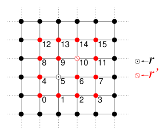
Figure 11: One of $N$ $4\times 4$ boxes used in the calculation of $S_{\Box}(\boldsymbol{r},\boldsymbol{r}^{\prime}-\boldsymbol{r}^{\prime\prime})$. Here, $\Box_{\boldsymbol{r}}$ has relative site labels 0 to 15 and is centered at site 5 with $\boldsymbol{r}^{\prime}$ currently located at site 10.

For the particular case shown in Fig. 11 with $\boldsymbol{r}^{\prime}=\boldsymbol{r}^{\prime}_{10}$ the matrix which contributes to the average $S_{\Box}(\boldsymbol{r},\boldsymbol{r}^{\prime}-\boldsymbol{r}^{\prime\prime})$ in Eq. (10) is written out explicitly as

$$S_{\Box}(\boldsymbol{r},\boldsymbol{r}^{\prime}-\boldsymbol{r}^{\prime\prime})=\cdots+\frac{\delta\rho_{10}}{16}\left(\begin{array}[]{cccc}\delta\rho_{14}+\delta\rho_{6}&\delta\rho_{5}+\delta\rho_{7}+\delta\rho_{13}+\delta\rho_{15}&2(\delta\rho_{4}+\delta\rho_{12})&\delta\rho_{5}+\delta\rho_{7}+\delta\rho_{13}+\delta\rho_{15}\\ 2\delta\rho_{2}&2(\delta\rho_{1}+\delta\rho_{3})&4\delta\rho_{0}&2(\delta\rho_{1}+\delta\rho_{3})\\ \delta\rho_{14}+\delta\rho_{6}&\delta\rho_{5}+\delta\rho_{7}+\delta\rho_{13}+\delta\rho_{15}&2(\delta\rho_{4}+\delta\rho_{12})&\delta\rho_{5}+\delta\rho_{7}+\delta\rho_{13}+\delta\rho_{15}\\ \delta\rho_{10}&\delta\rho_{9}+\delta\rho_{11}&2\delta\rho_{8}&\delta\rho_{9}+\delta\rho_{11}\end{array}\right)+\cdots$$ (17)

where we have employed the shorthand notation $\delta\rho_{i}\equiv\delta\rho(\boldsymbol{r}^{\prime}_{i})$. After performing the average over all $\boldsymbol{r}^{\prime}-\boldsymbol{r}^{\prime\prime}\in\Box_{\boldsymbol{r}}$ i.e. calculating all 16 matrices at each site, $S_{\Box}(\boldsymbol{r},\boldsymbol{r}^{\prime}-\boldsymbol{r}^{\prime\prime})$ is Fourier transformed over the relative coordinates in the box using Eq. (11) to give $S_{\Box}(\boldsymbol{r},\boldsymbol{k})$. This expression may then be evaluated at $\pm\boldsymbol{K}_{x}$ and $\pm\boldsymbol{K}_{y}$ using Eq. (12) to give the effective Ising-like order parameter $\widetilde{\Sigma}(\boldsymbol{r})$.

References

- (1) T. Hanaguri, C. Lupien, Y. Kohsaka, D.-H. Lee, M. Azuma, M. Takano, H. Takagi and J. C. Davis, Nature 430, 1001 (2004).
- (2) A. Fang, C. Howald, N. Kaneko, M. Greven, and A. Kapitulnik, Phys. Rev. B 70, 214514 (2004).
- (3) M. Vershinin, S. Misra, S. Ono, Y. Abe, Y. Ando, and A. Yazdani, Science 303, 1995 (2004).
- (4) K. McElroy, D.-H. Lee, J. E. Hoffman, K. M. Lang, E. W. Hudson, H. Eisaki, S. Uchida, J. Lee, and J. C. Davis, cond-mat/0404005.
- (5) A. Hashimoto, N. Momono, M. Oda, and M. Ido, cond-mat/0512496.
- (6) J.M. Tranquada, J.D. Axe, N. Ichikawa, A.R. Moodenbaugh, Y. Nakamura, and S. Uchida, Phys. Rev. Lett. 78, 338 (1997).
- (7) Y. Lee, R. Birgeneau, M. Kastner, Y. Endoh, S. Wakimoto, K. Yamada, R. Erwin, S. Lee, and G. Shirane, Phys. Rev. B 60, 3643 (1999).
- (8) J. M. Tranquada, H. Woo, T. G. Perring, H. Goka, G. D. Gu, G. Xu, M. Fujita, K. Yamada, Nature 429, 534 (2004).
- (9) P. Abbamonte, A. Rusydi, S. Smadici, G. D. Gu, G. A. Sawatzky, and D. L. Feng, Nature Physics 1, 155 (2005).
- (10) Spin Glasses and Random Fields, A. P. Young ed., World Scientific, Singapore (1997).
- (11) T. Nattermann, Phys. Rev. Lett. 64, 2454 (1990).
- (12) T. Giamarchi and P. Le Doussal, Phys. Rev. B 52, 1242 (1995).
- (13) C. Zeng, P. L. Leath, and D. S. Fisher, Phys. Rev. Lett. 82, 1935 (1999).
- (14) T. Nattermann and S. Scheidl, Adv. Phys. 49, 607 (2000).
- (15) A. Del Maestro and S. Sachdev, Phys. Rev. B 71, 184511 (2005).
- (16) M. Weigel and M. J. P. Gingras, cond-mat/0510614.
- (17) S. Kirkpatrick, C.D. Gelatt, and M.P. Vecchi, Science 220, 671 (1983).
- (18) J. R. Shewchuk, An Introduction to the Conjugate Gradient Method Without the Agonizing Pain (1994).
- (19) P. Siarry, G. Berthiau, F. Durbin and J. Haussy, ACM Trans. Math. Softw. 23, 209 (1997).
- (20) M. J. P. Gingras and D. A. Huse, Phys. Rev. B 53, 15193 (1996).
- (21) S. A. Kivelson, E. Fradkin, V. Oganesyan, I. Bindloss, J. Tranquada, A. Kapitulnik, and C. Howald, Rev. Mod. Phys. 75, 1201 (2003).
- (22) M. Vojta and S. Sachdev, cond-mat/0408461.
- (23) M. Vojta, T. Vojta, and R. K. Kaul, cond-mat/0510448.
- (24) J. Robertson, S. A. Kivelson, E. Fradkin, A. Fang, and A. Kapitulnik, cond-mat/0602675.