Fluctuation theorems for quantum master equations

Abstract

A quantum fluctuation theorem for a driven quantum subsystem interacting with its environment is derived based solely on the assumption that its reduced density matrix obeys a closed evolution equation i.e. a quantum master equation (QME). Quantum trajectories and their associated entropy, heat and work appear naturally by transforming the QME to a time dependent Liouville space basis that diagonalizes the instantaneous reduced density matrix of the subsystem. A quantum integral fluctuation theorem, a steady state fluctuation theorem and the Jarzynski relation are derived in a similar way as for classical stochastic dynamics.

I Introduction

The fluctuation theorems and the Jarzynski relation are some of a handful of powerful results of nonequilibrium statistical mechanics that hold far from thermodynamic equilibrium. Originally derived in the context of classical mechanics Jarzynski1 , the Jarzynski relation has been subsequently extended to stochastic dynamics Crooks0 . It relates the distribution of the work done by a driving force of arbitrary speed on a system initially at equilibrium (nonequilibrium property) to the free energy difference between the initial and final equilibrium state of the system (equilibrium property). This remarkable relation has recently been shown to hold for arbitrarily coupling strength between the system and the environment (see Jarzynski’s reply JarzynskiReply to criticism from Ref. Cohen ). The fluctuation theorems are based on a fundamental relation connecting the entropy production of a single system trajectory to the logarithm of the ratio of the probability of the forward and the backward trajectory Maes3 . The ensemble average of the trajectory entropy production is the macroscopic entropy production of the system whereas its distribution gives rise to various kinds of fluctuation theorems. The first has been derived for classical mechanics and initially for deterministic (but non-Hamiltonian) thermostated systems Evans1 ; Gallavotti ; Evans2 . Some interesting studies of fluctuation relations valid for far from equilibrium classical Hamiltonian systems have been made even earlier Bochkov ; Stratonovich ; JarsynskiFT . Fluctuation theorems for systems with stochastic dynamics have also been developed Kurchan1 ; Lebowitz ; Searles ; Gaspard1 ; Gaspard2 ; Crooks1 ; Crooks2 ; Seifert . For classical stochastic dynamics, the connection between the fluctuation theorem and the Jarzynski relation has been established by Crooks Crooks1 . Seifert has recently provided a unified description of the different fluctuation relations and of the Jarzynski relation for classical stochastic processes described by master equations Seifert .
The understanding of these two fundamental relations in quantum mechanics is still not fully established. Quantum Jarzynski relations have been investigated in HTasaki ; Yukawa ; Mukamel ; Maes . Quantum fluctuation theorems have been developed only in a few restricted situations Kurchan ; STasaki ; Maes1 ; Monnai . A quantum exchange fluctuation theorem has also been considered in JarzynskiQ . Some interesting considerations on the quantum definition of work in the previous studies have been made in Allahverdyan .
It should be noted that the dynamics of an isolated (whether driven or not) quantum system is unitary and its von Neumann entropy is time independent. Therefore, fluctuation theorems for such closed systems are useful only provided one defines some reduced macrovariable dynamics or some measurement process on the system Maes2 .

The purpose of this paper is to provide a unified derivation for the different quantum fluctuation relations (an integral fluctuation theorem, a steady state fluctuation theorem and the Jarzynski relation). We build upon the unification of the different fluctuation relations recently accomplished by Seifert Seifert for classical stochastic dynamics described by birth and death master equation (BDME). Quantum evolution involves coherences which make its interpretation in term of trajectories not obvious. Nevertheless, we show that it is possible to formally develop a trajectory picture of quantum dynamics which allows to uniquely represent entropy, heat and work distributions. This rely on the single assumption that the reduced dynamics of a driven quantum subsystem interacting with its environment is described by a closed evolution equation for the density matrix of the subsystem i.e. a QME Haake ; Spohn ; Gardiner ; Breuer . However, while the physical quantities defined along classical trajectories are conceptually clear and experimentally measurable, how to measure the physical quantities associated to quantum trajectories remains a fascinating open issue intimately connected to quantum measurement.

The plan of the paper is as follows: We start in section II by defining quantum heat and quantum work for a driven subsystem interacting with its environment in consistency with thermodynamics . We then discuss the consequences of defining heat and work in terms of the time dependent basis which diagonalizes the subsystem density matrix in section III. In section IV, we show that by assuming a QME for the subsystem reduced density matrix we can recast its solution in a representation which takes the form of a BDME with time dependent rates. In section V, we show that the BDME representation allows to split the entropy evolution in two parts, the entropy flow associated with exchange processes with the environment and the entropy production associated with subsystem internal irreversible processes. In section VI, we show that the BDME representation naturally allows to define quantum trajectories as well as their associated entropy flow and entropy production. We then derive the fundamental relation of this paper (67) which will allow us to derive, in section VII, a quantum integral fluctuation theorem and, in section VIII, a quantum steady state fluctuation theorem. Having identified in section IX the heat and the work associated to the quantum trajectories, we show in section X that the fundamental relation of section VI also allows to derive a quantum Jarzynski relation. We finally draw conclusions in section XI.

II Average heat and work

We start by defining the average quantum heat and work for a driven subsystem interacting with its environment and show the consistency of these definitions with thermodynamics . Heat and work can be rigorously expressed in term of the reduced density matrix of the subsystem without having to refer explicitly to the environment.

We consider a driven subsystem with Hamiltonian $\hat{H}_{S}(t)$. Everywhere in this paper we denote operators with an hat (and superators with two hats) and we use the Schrodinger picture where the time dependence of the observables is explicit and comes exclusively from external driving. We could also have written $\hat{H}_{S}(\lambda(t))$, where $\lambda(t)$ is the external time dependent driving. This subsystem is interacting with its environment whose Hamiltonian is $\hat{H}_{B}$. The interaction energy between the subsystem and the environment is described by $\hat{H}_{I}$. The Hamiltonian of the total system reads therefore

$$\hat{H}_{T}(t)=\hat{H}_{S}(t)+\hat{H}_{B}+\hat{H}_{I}\;.$$ (1)

We have assumed that the driving acts exclusively on the subsystem and does not affect $\hat{H}_{B}$ and $\hat{H}_{I}$.
The state of the total system is described by the density matrix $\hat{\rho}(t)$ which obeys the von Neumann equation

$$\dot{\hat{\rho}}(t)=-i[\hat{H}_{T}(t),\hat{\rho}(t)]=\hat{\hat{{\cal L}}}(t)\hat{\rho}(t)\;,$$ (2)

The energy of the total system is given by

$$\langle\hat{H}_{T}\rangle_{t}\equiv{\rm Tr}\hat{H}_{T}(t)\hat{\rho}(t)\;.$$ (3)

The change in the total energy between time $0$ and $t$ due to the time dependent driving is therefore given by

$$\Delta E_{T}(t)\equiv\int_{0}^{t}d\tau\frac{d\langle\hat{H}_{T}\rangle_{\tau}}{d\tau}=W_{T}(t)+Q_{T}(t)\;,$$ (4)

where the work and the heat have respectively been defined as

$$W_{T}(t)\equiv\int_{0}^{t}d\tau{\rm Tr}\dot{\hat{H}}_{T}(t)\hat{\rho}(t)$$ (5)

$$Q_{T}(t)\equiv\int_{0}^{t}d\tau{\rm Tr}\hat{H}_{T}(t)\dot{\hat{\rho}}(t)\;.$$ (6)

Using the von Neumann equation (2) and the invariance of the trace under cyclic permutation Comment , we find that no heat is generated in the isolated total system

$$Q_{T}(t)=-i\int_{0}^{t}d\tau{\rm Tr}\hat{H}_{T}(t)[\hat{H}_{T}(t),\hat{\rho}(t)]=0\;.$$ (7)

We next turn to the subsystem. Its reduced density matrix is defined as $\hat{\sigma}(t)\equiv{\rm Tr}_{B}\hat{\rho}(t)$ and its energy is given by

$$\langle\hat{H}_{S}\rangle_{t}\equiv{\rm Tr}\hat{H}_{S}(t)\hat{\rho}(t)={\rm Tr}_{S}\hat{H}_{S}(t)\hat{\sigma}(t)\;.$$ (8)

The change in this energy between time $0$ and $t$ is given by

$$\Delta E_{S}(t)\equiv\int_{0}^{t}d\tau\frac{d\langle\hat{H}_{S}\rangle_{\tau}}{d\tau}=W_{S}(t)+Q_{S}(t)\;,$$ (9)

where the work and the heat are defined as

$$W_{S}(t) \equiv \int_{0}^{t}d\tau{\rm Tr}\dot{\hat{H}}_{S}(\tau)\hat{\rho}_{T}(\tau)$$

$$= \int_{0}^{t}d\tau{\rm Tr}_{S}\dot{\hat{H}}_{S}(\tau)\hat{\sigma}(\tau)$$

$$Q_{S}(t) \equiv \int_{0}^{t}d\tau{\rm Tr}\hat{H}_{S}(\tau)\dot{\hat{\rho}}_{T}(\tau)$$

$$= \int_{0}^{t}d\tau{\rm Tr}_{S}\hat{H}_{S}(\tau)\dot{\hat{\sigma}}(\tau)\;.$$

Since the time dependence of the total system Hamiltonian comes solely from the subsystem Hamiltonian, $\dot{\hat{H}}_{B}=\dot{\hat{H}}_{I}=0$, $\dot{\hat{H}}_{T}=\dot{\hat{H}}_{S}$ and the work done by the driving force on the subsystem is the same as the work done by this force on the total system

$$W_{T}(t)=W_{S}(t)\equiv W(t)\;.$$ (12)

This also means that the energy increase in the subsystem minus the amount of heat which went to the environment is equal to the energy increase in the total system

$$W(t)=\Delta E_{T}(t)=\Delta E_{S}(t)-Q_{S}(t)\;.$$ (13)

It should be noticed that due to the absence of heat flux in the total system $Q_{T}(t)=0$, using (6) with (1) and (II), we can also express the heat going from the subsystem to the environment as

$$Q_{S}(t)=-\int_{0}^{t}d\tau\frac{d\langle\hat{H}_{B}\rangle_{\tau}}{d\tau}-\int_{0}^{t}d\tau\frac{d\langle\hat{H}_{I}\rangle_{\tau}}{d\tau}\;.$$ (14)

III Calculating heat and work in a time dependent basis

As will become clear in section IV, in order to associate trajectories to the quantum dynamics, one need to represent the dynamics in a time dependent basis. This is a fundamental difference from classical thermodynamics where the basis set (coordinate system) is fixed. In order to associate heat and work with single trajectories they must be defined with respect to the time dependent basis set. The ensemble average of the quantities defined for the trajectories will therefore also depend on the time dependent basis set. For this reason, we introduce a modified definition of heat and work. The effect of the basis time dependence on heat and work is given in appendix A.

The energy of the total system (3) can also be written as

$$\langle\hat{H}_{T}\rangle_{t}=\sum_{\alpha}P^{T}_{t}(\alpha)\langle\alpha_{t}|\hat{H}_{T}(t)|\alpha_{t}\rangle\;,$$ (15)

where we have introduced the time dependent basis $\{|\alpha_{t}\rangle\}$ which diagonalizes the instantaneous density matrix at all time

$$\langle\alpha_{t}|\hat{\rho}(t)|\alpha_{t}^{\prime}\rangle=\langle\alpha_{t}|\hat{\rho}(t)|\alpha_{t}\rangle\delta_{\alpha\alpha^{\prime}}\equiv P^{T}_{t}(\alpha)\delta_{\alpha\alpha^{\prime}}\;.$$ (16)

The change in this energy between time $0$ and $t$ due to the time dependent driving can therefore be rewritten as

$$\Delta E_{T}(t)=\tilde{W}_{T}(t)+\tilde{Q}_{T}(t)\;,$$ (17)

where the modified work and heat have respectively been defined as

$$\tilde{W}_{T}(t) \equiv \int_{0}^{t}d\tau\sum_{\alpha}P^{T}_{\tau}(\alpha)\frac{d}{d\tau}\bigg{(}\langle\alpha_{\tau}|\hat{H}_{T}(\tau)|\alpha_{\tau}\rangle\bigg{)}$$ (18)

$$\tilde{Q}_{T}(t) \equiv \int_{0}^{t}d\tau\sum_{\alpha}\dot{P}^{T}_{\tau}(\alpha)\langle\alpha_{\tau}|\hat{H}_{T}(\tau)|\alpha_{\tau}\rangle\;.$$ (19)

Because the total system is driven but otherwise isolated, its evolution is unitary and we have (see appendix A)

$$\tilde{W}_{T}(t) = W_{T}(t)=\Delta E_{T}(t)$$ (20)

$$\tilde{Q}_{T}(t) = Q_{T}(t)=0\;.$$ (21)

This means that defining heat and work on the time dependent basis which diagonalizes the instantaneous density matrix for unitary evolution is equivalent to the original definition of heat and work in a time independent basis.

The energy of the subsystem (9) can also be written in analogy to (15) as

$$\langle\hat{H}_{S}\rangle_{t}=\sum_{m}P_{t}(m)\langle m_{t}|\hat{H}_{S}(t)|m_{t}\rangle,$$ (22)

where we have introduced the time dependent basis $\{|m_{t}\rangle\}$ diagonalizing the instantaneous subsystem reduced density matrix

$$\langle m_{t}|\hat{\sigma}(t)|m_{t}^{\prime}\rangle=\langle m_{t}|\hat{\sigma}(t)|m_{t}\rangle\delta_{mm^{\prime}}\equiv P_{t}(m)\delta_{mm^{\prime}}\;.$$ (23)

Let us note for future reference that

$$\frac{d}{dt}(\langle m_{t}|\hat{\sigma}(t)|m_{t}^{\prime}\rangle) = \langle m_{t}|\dot{\hat{\sigma}}(t)|m_{t}^{\prime}\rangle$$

$$+\langle\dot{m}_{t}|\hat{\sigma}(t)|m_{t}^{\prime}\rangle+\langle m_{t}|\hat{\sigma}(t)|\dot{m}_{t}^{\prime}\rangle\;.$$

Eq. (23) and (III) give

$$\langle m_{t}|\dot{\hat{\sigma}}(t)|m_{t}^{\prime}\rangle = \dot{P}_{t}(m)\delta_{mm^{\prime}}$$

$$-\langle\dot{m}_{t}|m_{t}^{\prime}\rangle P_{t}(m^{\prime})-\langle m_{t}|\dot{m}_{t}^{\prime}\rangle P_{t}(m)\;.$$

Notice also that for $m=m^{\prime}$, we have

$$\langle m_{t}|\dot{\hat{\sigma}}(t)|m_{t}\rangle=\dot{P}_{t}(m)$$ (26)

because $\langle\dot{m}_{t}|m_{t}\rangle+\langle m_{t}|\dot{m}_{t}\rangle=\frac{d}{dt}(\langle m_{t}|m_{t}\rangle)=0$.
Using (22), the change in the subsystem energy between time $0$ and $t$ can be rewritten as

$$\Delta E_{S}(t)=\tilde{W}_{S}(t)+\tilde{Q}_{S}(t)\;,$$ (27)

where the work and the heat are defined in analogy to (18) and (19) as

$$\tilde{W}_{S}(t) \equiv \int_{0}^{t}d\tau\sum_{m}P_{\tau}(m)\frac{d}{d\tau}\bigg{(}\langle m_{\tau}|\hat{H}_{S}(\tau)|m_{\tau}\rangle\bigg{)}$$ (28)

$$\tilde{Q}_{S}(t) \equiv \int_{0}^{t}d\tau\sum_{m}\dot{P}_{\tau}(m)\langle m_{\tau}|\hat{H}_{S}(\tau)|m_{\tau}\rangle\;.$$ (29)

It is shown in appendix A that the work and heat defined in the time dependent basis $\{|m_{t}\rangle\}$ is related to the original work and heat defined in any time independent basis by

$$\tilde{W}_{S}(t) = W_{S}(t)+A_{S}(t)$$ (30)

$$\tilde{Q}_{S}(t) = Q_{S}(t)-A_{S}(t)\;,$$ (31)

where

$$A_{S}(t) \equiv \int_{0}^{t}d\tau\sum_{m}P_{\tau}(m)$$

$$\hskip 28.45274pt\bigg{(}\langle\dot{m}_{\tau}|\hat{H}_{S}(\tau)|m_{\tau}\rangle+\langle m_{\tau}|\hat{H}_{S}(\tau)|\dot{m}_{\tau}\rangle\bigg{)}\;.$$

It should be emphasized that both the original and the modified work and heat of the subsystem can be defined exclusively in term of the subsystem quantities without refering explicitly to the environment.
Using (12) and (13) with (30) and (31), we get

$$\Delta E_{T}(t) = W(t)=\tilde{W}_{S}(t)-A_{S}(t)$$

$$= \Delta E_{S}(t)-\tilde{Q}_{S}(t)-A_{S}(t)\;.$$

IV BDME representation of the QME solution

In this section we show that if we assume a closed evolution equation for the subsystem reduced density matrix, we can transform it solution in a BDME form with time dependent rates.

We assume that the reduced subsystem density matrix $\hat{\sigma}(t)$ obeys a closed QME. The literature on this topic is well furnished Haake ; Spohn ; Gardiner ; Breuer . This QME can be derived microscopically by perturbation theory like in the Redfield theory or using a quantum dynamical semigroups approach leading to Lindblad type master equations. In Liouville space MukamelB , the QME of the externally driven subsystem interacting with its environment reads

$$|\dot{\hat{\sigma}}(t)\gg=\hat{\hat{{\cal K}}}(t)|\hat{\sigma}(t)\gg\;.$$ (34)

If the interaction with the environment vanishes, the generator $\hat{\hat{{\cal K}}}(t)$ becomes the antihermitian superoperator $\hat{\hat{{\cal K}}}(t)=\hat{\hat{{\cal L}}}_{S}(t)=-{\rm i}[\hat{H}_{S}(t),\cdot]$ and the evolution superoperator $\hat{\hat{{\cal M}}}_{t}$ defined by $|\hat{\sigma}(t)\gg=\hat{\hat{{\cal M}}}_{t}|\hat{\sigma}(0)\gg$ becomes the unitary superoperator $\hat{\hat{{\cal M}}}_{t}=\exp_{+}{\{\int_{0}^{t}d\tau\hat{\hat{{\cal L}}}_{S}(\tau)\}}$. However, for non vanishing coupling this generator is not antihermician and leads to a nonunitary evolution.
The QME in some given (possibly time dependent) basis reads

$$\ll ii^{\prime}|\dot{\hat{\sigma}}(t)\gg=\sum_{jj^{\prime}}\ll ii^{\prime}|\hat{\hat{{\cal K}}}(t)|jj^{\prime}\gg\ll jj^{\prime}|\hat{\sigma}(t)\gg\;,$$ (35)

where $\ll jj^{\prime}|\hat{\sigma}(t)\gg$ is the superoperator representation of $\langle j|\hat{\sigma}(t)|j^{\prime}\rangle$. Let us now use the time dependent basis $\{|m_{t}\rangle\}$ introduced in (23). Since the QME keeps $\hat{\sigma}(t)$ hermitian, this diagonalization is always possible.

$$\ll m_{t}m_{t}^{\prime}|\hat{\sigma}(t)\gg=P_{t}(m)\delta_{m,m^{\prime}}\;.$$ (36)

A crucial property of this basis is that [see Eq. (26)]

$$\dot{P}_{t}(m)=\ll m_{t}m_{t}|\dot{\hat{\sigma}}(t)\gg\;.$$ (37)

The consequence of this property is that by defining

$$W_{t}(m^{\prime},m) \equiv \ll m_{t}m_{t}|\hat{\hat{{\cal K}}}(t)|m_{t}^{\prime}m_{t}^{\prime}\gg\;,$$ (38)

and by projecting the QME (34) on the time dependent superbra $\ll m(t)m(t)|$ we get

$$\dot{P}_{t}(m)=\sum_{m^{\prime}}W_{t}(m^{\prime},m)P_{t}(m^{\prime})\;.$$ (39)

Since the QME (34) preserves probability, we have $\sum_{m}W_{t}(m^{\prime},m)=0$ and $W_{t}(m^{\prime},m)$ real. Therefore, we can rewrite (39) as

$$\dot{P}_{t}(m)=\sum_{m^{\prime}\neq m}\{W_{t}(m^{\prime},m)P_{t}(m^{\prime})-W_{t}(m,m^{\prime})P_{t}(m)\}\;.$$ (40)

This equation appears like a BDME but should not be viewed as an equation of motion. It is merely a way of recasting the solution of the QME (34) in a diagonal basis. In fact, in order to get the $P_{t}(m)$’s and the $W_{t}(m^{\prime},m)$’s, we need to solve the QME first and find the time dependent unitary transformation diagonalizing the solution $\hat{\sigma}(t)$ at any time. Eq. (39) should therefore be viewed as a formal definition of the rate matrix $W_{t}(m^{\prime},m)$. We will show that $W_{t}(m^{\prime},m)$ defined in this way can be used to derive quantum fluctuation relations. Note that $W_{t}(m^{\prime},m)$ depends on the subsystem initial condition $\hat{\sigma}(0)$.

If the subsystem (driven or not) does not interact with the environment, the generator is antihermician and the evolution superoperator unitary. In this case $|\hat{\sigma}(t)\gg=\hat{\hat{{\cal M}}}_{t}\;|\hat{\sigma}(0)\gg$ and $\ll m_{t}m_{t}|=\ll m_{0}m_{0}|\;\hat{\hat{{\cal M}}}^{-1}_{t}$, so that

$$P_{t}(m)=\langle m_{0}|\hat{\sigma}(0)|m_{0}\rangle=P_{0}(m)\;.$$ (41)

This shows that the $P_{t}(m)$’s evolve only if the dynamics is nonunitary.
When there is no driving and the subsystem does interact with its environment, the dynamics is nonunitary and the subsystem will reach equilibrium $\hat{\sigma}^{\rm eq}$ on long time scales. For an infinite isothermal environment this equilibrium state will correspond to the canonical subsystem reduced density matrix $\hat{\sigma}^{\rm eq}={\rm e}^{-\beta\hat{H}_{S}}/Z_{S}$ where $Z_{S}={\rm Tr}\;{\rm e}^{-\beta\hat{H}_{S}}$ and $\beta=1/T$ ($k_{B}\equiv 1$). In this case the basis diagonalizing $\hat{\sigma}^{\rm eq}$ becomes time independent and will also diagonalize the subsystem Hamiltonian so that $P^{\rm eq}(m)=e^{-\beta E_{m}}/Z_{S}$ where $E_{m}$ are the eigenvalues of the subsystem Hamiltonian.
For a subsystem with nonequilibrium boundary conditions and interacting with its environment, the subsystem can reache a steady state $\hat{\sigma}^{\rm st}$ on long times. In this case the matrix diagonalizing the density matrix is again time independent and both the probabilities $P_{t}(m)=P^{\rm st}(m)$ and the rates $W_{t}(m^{\prime},m)=W^{\rm st}(m^{\prime},m)$ become time independent.

V Entropy for quantum ensembles

In this section we define the von Neumann entropy associated with the subsystem and separate its evolution into two parts: the entropy flow associated to the heat going from the subsystem to the environment and the entropy production associated to the internal (always positive) entropy growth of the subsystem.

The von Neumann entropy of the subsystem is defined by

$$S(t)\equiv-{\rm Tr}\;\hat{\sigma}(t)\ln\hat{\sigma}(t)=-\sum_{m}P_{t}(m)\ln P_{t}(m)$$ (42)

Using Eq. (40), we can write its time derivative as

$$\dot{S}(t) = -\sum_{m}\dot{P}_{t}(m)\ln P_{t}(m)$$ (43)

$$= -\sum_{m,m^{\prime}}P_{t}(m)W_{t}(m,m^{\prime})\ln\frac{P_{t}(m^{\prime})}{P_{t}(m)}$$ (44)

In analogy with Lebowitz ; Gaspard1 for classical systems, this can be partitioned as

$$\dot{S}(t)=\dot{S}_{e}(t)+\dot{S}_{i}(t)\;,$$ (45)

where

$$\dot{S}_{e}(t)\equiv-\sum_{m,m^{\prime}}P_{t}(m)W_{t}(m,m^{\prime})\ln\frac{W_{t}(m,m^{\prime})}{W_{t}(m^{\prime},m)}\;,$$ (46)

and where

$$\dot{S}_{i}(t)\equiv\sum_{m,m^{\prime}}P_{t}(m)W_{t}(m,m^{\prime})\ln\frac{P_{t}(m)W_{t}(m,m^{\prime})}{P_{t}(m^{\prime})W_{t}(m^{\prime},m)}\;.$$ (47)

As a consequence of the inequality $(R_{1}-R_{2})\ln(R_{1}/R_{2})\geq 0$, we notice that $\dot{S}_{i}(t)\geq 0$ is an always positive quantity. We will therefore identify it with the entropy production. The remaining part of the entropy $\dot{S}_{e}(t)$ is thus associated with the entropy flow to the environment since in thermodynamics the entropy evolution is partitioned in the (reversible) entropy flow to the environment and the (irreversible) entropy production GrootMazur ; Prigogine . To further rationalize this identification, let us assume that $W_{t}(m,m^{\prime})$ satisfy the detailed balance condition Crooks1 ; Kampen ; GrootMazur . For isothermal environments at temperature $T$, the detailed balance condition with respect to $\hat{H}_{s}(t)$, which means that the non-driven subsystem tends to thermal equilibrium at long time, reads

$$\frac{W_{t}(m,m^{\prime})}{W_{t}(m^{\prime},m)}={\rm e}^{\beta\left(\langle m_{t}|\hat{H}_{S}(t)|m_{t}\rangle-\langle m_{t}^{\prime}|\hat{H}_{S}(t)|m_{t}^{\prime}\rangle\right)}\;.$$ (48)

Noticing that the heat (29) can be rewritten as

$$\dot{\tilde{Q}}(t) = \sum_{m}\dot{P}_{t}(m)\langle m_{t}|\hat{H}_{S}(t)|m_{t}\rangle$$

$$= -\sum_{m,m^{\prime}}P_{t}(m)W_{t}(m,m^{\prime})$$

$$\hskip 28.45274pt\left(\langle m_{t}|\hat{H}_{S}(t)|m_{t}\rangle-\langle m_{t}^{\prime}|\hat{H}_{S}(t)|m_{t}^{\prime}\rangle\right)$$

$$= -T\sum_{m,m^{\prime}}P_{t}(m)W_{t}(m,m^{\prime})\ln\frac{{\rm e}^{\beta\langle m_{t}|\hat{H}_{S}(t)|m_{t}\rangle}}{{\rm e}^{\beta\langle m_{t}^{\prime}|\hat{H}_{S}(t)|m_{t}^{\prime}\rangle}}$$

and using (46), the immediate consequence of (48) is that the entropy flow is equal to the modified heat going from the subsystem to the environment divided by the environment temperature as expected from thermodynamics

$$\dot{S}_{e}(t)=\frac{\dot{\tilde{Q}}_{S}}{T}\;.$$ (50)

This motivates our partition of the entropy (45) and the definition of the modified heat in section III.

We can further show that the entropy flow is associated to reversible entropy variations. In the thermodynamical sense, a reversible transformation is a one during which the entropy production is zero $\dot{S}_{i}(t)=0$. This property holds provided the following condition is satisfied [see (47)]

$$P_{t}(m)W_{t}(m,m^{\prime})=P_{t}(m^{\prime})W_{t}(m^{\prime},m)\;.$$ (51)

Using now Eq.(48), we find that for a reversible transformation the subsystem has to be at all time in the time dependent state

$$P_{t}(m)=\frac{{\rm e}^{-\beta\langle m_{t}|\hat{H}_{S}(t)|m_{t}\rangle}}{\sum_{m}{\rm e}^{-\beta\langle m_{t}|\hat{H}_{S}(t)|m_{t}\rangle}}\;.$$ (52)

This state correspond to the instantaneous Gibbs state of the subsystem $\hat{\sigma}(t)={\rm e}^{-\beta\hat{H}_{S}(t)}/Z_{S}$. In this case $\{|m\rangle_{t}\}$ in Eq.(51) becomes the adiabatic basis (basis diagonalizing the subsystem Hamiltonian). We thus show that for reversible transformations the probability distribution remains Gibbsian along the adiabatic levels. Because $\dot{S}_{i}(t)=0$, we also have $\dot{S}(t)=\dot{S}_{e}(t)$. Using (48), this means that for a reversible transformation the change in the entropy of the subsystem result exclusively from the heat flow to the environment $\dot{S}(t)=\dot{\tilde{Q}}_{S}/T$ in consistency with thermodynamics.
When there is no driving, Eq. (51) with Eq. (48) define equilibrium. At equilibrium we have $\dot{S}(t)=\dot{S}_{i}(t)=\dot{S}_{e}(t)=0$.

VI Entropy for quantum trajectories

In this section we introduce quantum trajectories and distributions. We will associate an entropy with these trajectories and identify the entropy flow and production of these trajectories whose ensemble averages recover the entropies discussed in section V. This will allow us to derive a fundamental quantum relation similar to the classical relation obtained by Crooks Crooks1 and Seifert Seifert connecting the ratio of the probability of a forward trajectory and the ”backward” one with the trajectory entropy production.

From Eq. (40) it seems natural to unravel the evolution equation for the probability $P_{t}(m)$ in the same way as is done for classical stochastic processes Seifert . Let us consider a stochastic trajectory of duration $t$ which contains $N$ jumps. Different trajectories can of course have a different number of jumps $N$. $\tau=[0,t]$ labels time during the process. $j=1,\ldots,N$ labels the jumps. The trajectory $n_{(\tau)}$ [see Fig. 1] is made by the successive states taken by the system in time

$$n_{(\tau)}=n_{0}\to n_{1}\to n_{2}\to\ldots\to n_{N}\;.$$ (53)

The system starts in $n_{0}$, jumps at time $\tau_{j}$ from $n_{j-1}$ to $n_{j}$ and ends up at time $t$ in $n_{N}$. We will denote $\tau_{0}=0$ and $\tau_{N+1}=t$.

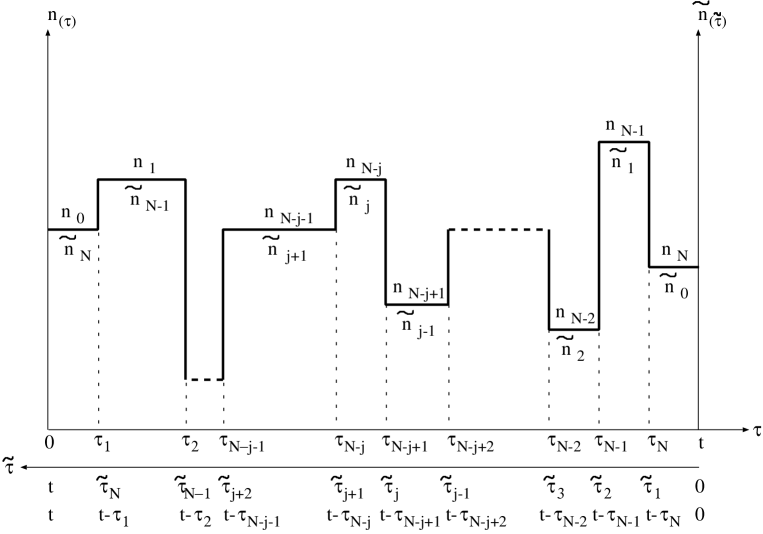
Figure 1: Representation of a quantum forward trajectory $n_{(\tau)}$ and of the associated pseudo-backward trajectory $\tilde{n}_{(\tilde{\tau})}$.

The entropy associated with the trajectory $n_{(\tau)}$ reads

$$s(\tau)\equiv-\ln P_{\tau}(n_{(\tau)})\;,$$ (54)

where $P_{\tau}(n_{(\tau)})$ is the solution of Eq. (40) for an initial condition $P_{0}(n_{0})$ evaluated along the trajectory $n_{(\tau)}$.
The time derivative of this trajectory entropy

$$\dot{s}(\tau)=-\frac{\partial_{\tau}P_{\tau}(n)}{P_{\tau}(n)}|_{n_{(\tau)}}-\sum_{j=1}^{N}\delta(\tau-\tau_{j})\ln\frac{P_{\tau}(n_{j})}{P_{\tau}(n_{j-1})}\;,$$ (55)

will be separated as

$$\dot{s}(\tau)=\dot{s}_{e}(\tau)+\dot{s}_{i}(\tau)\;,$$ (56)

where the trajectory entropy flux reads

$$\dot{s}_{e}(\tau)\equiv-\sum_{j=1}^{N}\delta(\tau-\tau_{j})\ln\frac{W_{\tau}(n_{j-1},n_{j})}{W_{\tau}(n_{j},n_{j-1})}$$ (57)

and the trajectory entropy production reads

$$\dot{s}_{i}(\tau) \equiv -\frac{\partial_{t}P_{\tau}(n)}{P_{\tau}(n)}|_{n_{(\tau)}}$$

$$-\sum_{j=1}^{N}\delta(\tau-\tau_{j})\ln\frac{P_{\tau}(n_{j})W_{\tau}(n_{j},n_{j-1})}{P_{\tau}(n_{j-1})W_{\tau}(n_{j-1},n_{j})}\;.$$

The ensemble average over the different trajectories is carried out by using the probability $P_{\tau}(n_{j-1})W_{\tau}(n_{j-1},n_{j})$ that a transition occurs at time $\tau_{j}$ between $n_{j-1}$ and $n_{j}$. We get

$$\dot{S}(\tau) = \langle\dot{s}(\tau)\rangle$$ (59)

$$\dot{S}_{e}(\tau) = \langle\dot{s}_{e}(\tau)\rangle$$ (60)

$$\dot{S}_{i}(\tau) = \langle\dot{s}_{i}(\tau)\rangle$$ (61)

The probability of a forward trajectory $n_{(\tau)}$ starting at time $0$ and ending at time $t$ is given by

$$\mu_{F}[n_{(\tau)}] = P_{0}(n_{0})$$

$$\left[\prod_{j=1}^{N}\exp{\left(-\int_{\tau_{j-1}}^{\tau_{j}}d\tau^{\prime}\sum_{m}W_{\tau^{\prime}}(n_{j-1},m)\right)}W_{\tau_{j}}(n_{j-1},n_{j})\right]$$

$$\hskip 25.6073pt\exp{\left(-\int_{\tau_{N}}^{t}d\tau^{\prime}\sum_{m}W_{\tau^{\prime}}(n_{N},m)\right)}\;.$$

The exponentials represent the probabilities to stay in a given state during the time interval between two successive jumps, and the transition rates evaluated at the jump times give the probability for the jumps to occur at this given times.

Defining the backward process as done for classical stochastic dynamics Seifert is not possible. In the classical case, it is sufficient after the forward process to revert the driving protocol $\tilde{\lambda}(\tau)=\lambda(t-\tau)$ and to ask for the probability of a backward trajectory (system taking the sequence of states of the forward trajectory but in the reversed order) to occur. The reversal of the driving protocol has the consequence of reversing the time dependence of the transition matrix $\tilde{W}_{\tau}(m,m^{\prime})=W_{t-\tau}(m,m^{\prime})$ so that the backward process clearly correspond to a physical process. However, the time dependence of the quantum transition matrix $W_{t}(m,m^{\prime})$ does not come exclusively from the external driving force and is different for different initial conditions of the subsystem $\hat{\sigma}(0)$. Therefore, reversing the driving protocol does not simply reverse the time dependence of the transition matrix. Nevertheless, in order to have a process corresponding to a reversal of the time dependence of the transition matrix, we will formally define an artificial backward process. This definition will allow us to derive important fluctuation relations in next sections.
Let us consider a new dynamics in the time interval $\tilde{\tau}=[0,t]$ obeying

$$\dot{\tilde{P}}_{\tilde{\tau}}(m)=\sum_{\tilde{m}^{\prime}}\tilde{W}_{\tilde{\tau}}(\tilde{m}^{\prime},\tilde{m})\tilde{P}_{\tilde{\tau}}(\tilde{m}^{\prime})\;,$$ (63)

where the rates are related to the previous rates in the following way

$$\tilde{W}_{\tilde{\tau}}(\tilde{m}^{\prime},\tilde{m})=W_{t-\tilde{\tau}}(\tilde{m}^{\prime},\tilde{m})\;.$$ (64)

Let us call this dynamics with an arbitrary initial condition $\tilde{P}_{0}(\tilde{n}_{0})$ the pseudo-backward dynamics. This dynamic does not correspond in general to a quantum dynamics as (39). We define now the following trajectory for this pseudo-backward dynamics

$$\tilde{n}_{(\tilde{\tau})} = \tilde{n}_{0}\to\tilde{n}_{1}\to\tilde{n}_{2}\to\ldots\to\tilde{n}_{N}$$ (65)

$$= n_{N}\to n_{N-1}\to n_{N-2}\to\ldots\to n_{0}\;.$$

where the jumps between $\tilde{n}_{j-1}$ and $\tilde{n}_{j}$ occur at time $\tilde{\tau}_{j}=t-\tau_{N-j+1}$ and where $\tilde{n}_{j}=n_{N-j}$. Because this dynamics as well as the dynamics (40) both span the same configuration space, summing over all trajectories of the pseudo-backward process is equivalent to summing over all the trajectories of the original process. The trajectory (65) is depicted on Fig. 1. The forward probability of this trajectory is evaluated in appendix B and reads

$$\tilde{\mu}_{F}[\tilde{n}_{(\tilde{\tau})}] = \tilde{P}_{0}(n_{N})$$

$$\bigg{[}\prod_{j=1}^{N}\exp{\left(-\int_{\tau_{j-1}}^{\tau_{j}}d\tau^{\prime}\sum_{m}W_{\tau^{\prime}}(n_{j-1},m)\right)}$$

$$W_{\tau_{j}}(n_{j},n_{j-1})\bigg{]}\exp{\left(-\int_{\tau_{N}}^{t}d\tau^{\prime}\sum_{m}W_{\tau^{\prime}}(n_{N},m)\right)}\;.$$

We now consider the ratio of the forward (VI) and pseudo-backward (VI) probability. Noticing that the exponentials cancels, we find the fundamental result of the paper

$$r(t)=\ln\frac{\mu_{F}[n_{(\tau)}]}{\tilde{\mu}_{F}[\tilde{n}_{(\tilde{\tau})}]}=\ln\frac{P_{0}(n_{0})}{\tilde{P}_{0}(n_{N})}-\Delta s_{e}(t)\;,$$ (67)

where the trajectory entropy flow is

$$\Delta s_{e}(t) \equiv s_{e}(t)-s_{e}(0)=\int_{0}^{t}d\tau\dot{s}_{e}(\tau)$$ (68)

$$= \sum_{j=1}^{N}\ln\frac{W_{\tau_{j}}(n_{j},n_{j-1})}{W_{\tau_{j}}(n_{j-1},n_{j})}\;.$$

In analogy with the classical results of Seifert Seifert , we can now derive the various fluctuation theorems by specific choices of initial conditions for the pseudo-backward trajectories. By choosing $\tilde{P}_{0}(n_{N})=P_{t}(n_{N})$ and using the trajectory entropy

$$\Delta s(t)\equiv s(t)-s(0)=\ln\frac{P_{0}(n_{0})}{P_{t}(n_{N})}\;,$$ (69)

Eq. (67) becomes

$$r(t)=\ln\frac{\mu_{F}[n_{(\tau)}]}{\tilde{\mu}_{F}[\tilde{n}_{(\tilde{\tau})}]}=\Delta s(t)-\Delta s_{e}(t)=\Delta s_{i}(t)$$ (70)

where $\Delta s_{i}(t)=s_{i}(t)-s_{i}(0)$ is the trajectory entropy production.

Eq. (67) has been first derived by Crooks Crooks1 for classical stochastic processes and later generalized by others Seifert ; Maes3 . We have shown that this relation may be extended to quantum systems. The pseudo-backward trajectories are artificial. In the classical case, because the time dependence of the rates is exclusively due to the external driving, the backward process has a physical meaning (e.g. Seifert ). However, in the quantum case the time dependence of the rates is also due to the quantum evolution of the density matrix itself, preventing us from associating in general a physical process to the backward dynamics.

VII Quantum integral fluctuation theorem

Summing over all possible trajectories of the pseudo-backward process is equivalent to summing over all possible trajectories of the original process $\sum_{\tilde{n}_{(\tilde{\tau})}}=\sum_{n_{(\tau)}}$. By averaging (67) over all possible trajectories, we find

$$1 = \sum_{\tilde{n}_{(\tilde{\tau})}}\tilde{\mu}_{F}[\tilde{n}_{(\tilde{\tau})}]=\sum_{n_{(\tau)}}\tilde{\mu}_{F}[\tilde{n}_{(\tilde{\tau})}]$$ (71)

$$= \sum_{n_{(\tau)}}\mu_{F}[n_{(\tau)}]e^{-r(t)}=\langle e^{-r(t)}\rangle\;.$$

This integral fluctuation theorem Seifert is valid for any choice of $P_{0}(n_{0})$ and $\tilde{P}_{0}(n_{N})$ in (67). Using the fact that $\langle e^{x}\rangle\geq e^{\langle x\rangle}$ this relation also means that in average the quantity $r(t)$ is always non-negative $\langle r(t)\rangle\geq 0$. Choosing $\tilde{P}_{0}(n_{N})=P_{t}(n_{N})$ we have $r(t)=\Delta s_{i}(t)$ and we show again [see text below (47)] that the ensemble averaged trajectory entropy production is always non-negative $\langle\Delta s_{i}(t)\rangle\geq 0$.

VIII Quantum fluctuation theorem for steady state

We consider a subsystem which is subjected to nonequilibrium constraints and we assume that its dynamics can be described by a QME of the form (34). When the subsystem is in a steady state, its density matrix does not evolve in time and the rates in equation (40) are time independent. An example of such system could be a two-level atom driven by a coherent single mode field on resonance (in the dipole approximation and in the rotating wave approximation) described by Bloch equations (see p154 of Ref. Breuer ). In a steady state, the pseudo-backward process introduced in section VI would correspond to the real physical backward process

$$\tilde{\mu}_{F}[\tilde{n}_{(\tilde{\tau})}]=\mu_{B}[n_{(\tau)}]\;.$$ (72)

By definition, we have

$$p_{F}(R(t)) = \langle\delta(R(t)-r_{F}(t))\rangle_{F}$$

$$= \sum_{n_{(\tau)}}\mu_{F}[n_{(\tau)}]\delta(R(t)-r_{F}(t))$$

Using (67), we can write

$$p_{F}(R(t)) = \sum_{n_{(\tau)}}\mu_{B}[n_{(\tau)}]e^{r_{F}(t)}\delta(R(t)-r_{F}(t))$$ (73)

$$= \sum_{n_{(\tau)}}\mu_{B}[n_{(\tau)}]e^{R(t)}\delta(R(t)-r_{F}(t))$$

$$= \langle\delta(R(t)+r_{B}(t))\rangle_{B}\;e^{R(t)}$$

$$= p_{B}(-R(t))\;e^{R(t)}\;,$$

where to go from the second line to the third one, we used $r_{F}(t)=-r_{B}(t)$ which comes from (72) with (67). When $\tilde{P}_{0}(n_{N})=P_{t}(n_{N})$ and therefore Eq. (70) holds, Eq. (73) becomes a fluctuation theorem for the entropy production

$$p_{F}(\Delta S_{i}(t))=p_{B}(-\Delta S_{i}(t))\;e^{\Delta S_{i}(t)}$$ (74)

This relation shows that at steady state, the ratio of the probability to observe a given entropy production during a froward process and the probability to observe the same entropy production with a minus sign during the backward process is given by the exponential of the entropy production. This is the most familiar form of the fluctuation theorem. In the infinite time limit, if the subsystem as a finite number of levels (this condition is usually implicitly assumed in QME theory) $\Delta S(t)$ will be bounded and $\Delta S_{i}(t)\stackrel{{\scriptstyle t\to\infty}}{{=}}\Delta S_{e}(t)$ so that (74) also becomes a fluctuation theorem for the entropy flow and therefore also for the heat. For completeness, we give in appendix C a different derivation of a fluctuation theorem similar to (74) and which is not restricted to steady states.

IX Heat and work for quantum trajectories

If we use the relation (48) together with the definition of the trajectory entropy flow (68), we find that the heat associated with a single trajectory is given by

$$\tilde{q}_{S}(t) \equiv \beta^{-1}\Delta s_{e}(t)$$

$$= \sum_{j=1}^{N}\left(\langle n_{j}|\hat{H}_{S}(\tau_{j})|n_{j}\rangle-\langle n_{j-1}|\hat{H}_{S}(\tau_{j})|n_{j-1}\rangle\right)\;.$$

The interpretation of this result is that the heat flowing to the environment results from transitions between the subsystem states $n_{j}$.
The energy associated with a trajectory is a state function and only depends on the initial and final state of the trajectory

$$\Delta e_{S}(t) = \langle n_{N}|\hat{H}_{S}(t)|n_{N}\rangle-\langle n_{0}|\hat{H}_{S}(0)|n_{0}\rangle$$ (76)

$$= \sum_{j=1}^{N}\left(\langle n_{j}|\hat{H}_{S}(\tau_{j})|n_{j}\rangle-\langle n_{j-1}|\hat{H}_{S}(\tau_{j})|n_{j-1}\rangle\right)$$

$$= \tilde{w}_{S}(t)+\tilde{q}_{S}(t)\;.$$

The work is therefore given by

$$\tilde{w}_{S}(t) = \Delta e_{S}(t)-\tilde{q}_{S}(t)$$

$$=\sum_{j=1}^{N}\left(\langle n_{j-1}|\hat{H}_{S}(\tau_{j})|n_{j-1}\rangle-\langle n_{j-1}|\hat{H}_{S}(\tau_{j-1})|n_{j-1}\rangle\right)\;.$$

The work thus results from the time evolution of the Hamiltonian (due to the driving force) along the states $n_{j}$ of the subsystem between the transitions. It is interesting to make the parallel between our description of heat and work in the $\{|m_{t}\rangle\}$ basis set and the adiabatic basis description of Ref. Mukamel . In the latter the work comes from the evolution along the adiabatic states and the heat comes from the transitions between the adiabatic state. This can be understood by comparing (A) and (A) with (A) and (A).

X The quantum Jarzynski relation

We assume that the subsystem is initially at equilibrium with respect to the Hamiltonian $\hat{H}_{S}(0)=\hat{H}_{S}(\lambda(0))$ and is therefore described by a canonical distribution. The system is then driven out of equilibrium by turning the driving force from $\lambda(0)$ to $\lambda(t^{\prime})$ at time $t^{\prime}$. After $t^{\prime}$ the driving force stop evolving. On long time scales after $t^{\prime}$, say $t$ ($t\gg t^{\prime}$), the system is again at equilibrium in a canonical distribution but now with respect to $\hat{H}_{S}(t)=\hat{H}_{S}(\lambda(t))$.
We choose

$$P_{0}(n_{0}) = \frac{e^{-\beta\langle n_{0}|\hat{H}_{S}(0)|n_{0}\rangle}}{Z_{0}}$$

$$P_{t}(n_{N}) = \frac{e^{-\beta\langle n_{N}|\hat{H}_{S}(t)|n_{N}\rangle}}{Z_{t}}\;,$$ (78)

where $Z_{0}=\sum_{n}\exp{(-\beta\langle n_{0}|\hat{H}_{S}(0)|n_{0}\rangle)}$ and $Z_{t}=\sum_{n}\exp{(-\beta\langle n_{N}|\hat{H}_{S}(t)|n_{N}\rangle)}$. Notice that $\{|n_{0}\rangle\}$ [$\{|n_{t}\rangle\}$] is now the eigenbasis of $\hat{H}_{S}(0)$ [$\hat{H}_{S}(t)$].
The free energy difference between the initial and the final state is given by

$$\Delta F(t)=F(t)-F(0)=-\beta^{-1}\ln\frac{Z_{t}}{Z_{0}}\;.$$ (79)

Using Eq. (IX) which defines the heat of a single subsystem trajectory, we can write Eq. (70) as

$$\Delta s_{i}(t) = -\ln P_{t}(n_{N})+\ln P_{0}(n_{0})-\beta\tilde{q}_{S}(t)\;.$$ (80)

Using now (78), (79), (76) and (IX), we can rewrite (80) as

$$\Delta s_{i}(t) = -\beta\Delta F(t)+\beta\tilde{w}_{S}(t)\;.$$ (81)

Finally, by inserting Eq. (81) in the integral fluctuation theorem (71) where $r(t)=\Delta s_{i}(t)$, we find the quantum Jarzynski relation

$$e^{-\beta\Delta F(t)}=\langle e^{-\beta\tilde{w}_{S}(t)}\rangle\;.$$ (82)

XI Conclusions

We have presented a unified derivation of a quantum integral fluctuation theorem, a quantum steady state fluctuation theorem, and the quantum Jarzynski relation, for a driven subsystem interacting with its environment and described by a QME. This generalizes earlier results obtained for quantum systems. By recasting the solution of the QME in a BDME form with time dependent rate for the eigenvalues of the subsystem density matrix, we naturally define quantum trajectories and their associated entropy, heat and work and study their fluctuation properties. The connection between the trajectory quantities which naturally enter our formulation and measurable quantum trajectory quantities is still an open issue. Deriving quantum fluctuation relations without having to assume QME, which do not correctly account for strong subsystem-environment entanglement, is an exiting perspective.

Appendix A Basis dependence of heat and work

We consider a system with a time dependent Hamiltonian $\hat{H}(t)$ in the Schrodinger picture described by the density matrix $\hat{\rho}(t)$. The evolution equation of $\hat{\rho}(t)$ is not necessarily unitary.
The energy of the system is given by

$$\langle\hat{H}\rangle\equiv{\rm Tr}\hat{H}(t)\hat{\rho}(t)=\sum_{aa^{\prime}}\langle a_{t}|\hat{H}(t)|a_{t}^{\prime}\rangle\langle a_{t}^{\prime}|\hat{\rho}(t)|a_{t}\rangle\;,$$ (83)

where $\{|a_{t}\rangle\}$ is an arbitrary time dependent basis set. The energy changes of the system can be written as

$$\Delta E(t) \equiv \int_{0}^{t}d\tau\frac{d\langle\hat{H}(\tau)\rangle}{d\tau}$$

$$= W(t)+Q(t)=\tilde{W}(t)+\tilde{Q}(t)$$

where the heat and the work are given by

$$\dot{Q}(t) \equiv {\rm Tr}\hat{H}(t)\dot{\hat{\rho}}(t)$$ (85)

$$\dot{W}(t) \equiv {\rm Tr}\dot{\hat{H}}(t)\hat{\rho}(t)\;,$$ (86)

in a time independent basis and by

$$\dot{\tilde{Q}}(t) \equiv \sum_{aa^{\prime}}\langle a_{t}|\hat{H}(t)|a_{t}^{\prime}\rangle\frac{d}{dt}\bigg{(}\langle a_{t}^{\prime}|\hat{\rho}(t)|a_{t}\rangle\bigg{)}$$ (87)

$$\dot{\tilde{W}}(t) \equiv \sum_{aa^{\prime}}\frac{d}{dt}\bigg{(}\langle a_{t}|\hat{H}(t)|a_{t}^{\prime}\rangle\bigg{)}\langle a_{t}^{\prime}|\hat{\rho}(t)|a_{t}\rangle\;,$$ (88)

in a time dependent basis.
How does $Q(t)$ [$W(t)$] relates to $\tilde{Q}(t)$ [$\tilde{W}(t)$]? We find

$$\dot{\tilde{Q}}(t) = \dot{Q}(t)-\dot{A}(t)$$ (89)

$$\dot{\tilde{W}}(t) = \dot{W}(t)+\dot{A}(t)\;,$$

where

$$\dot{A}(t) = -\sum_{aa^{\prime}}\langle a_{t}|\hat{H}(t)|a_{t}^{\prime}\rangle\bigg{(}\langle\dot{a}_{t}^{\prime}|\hat{\rho}(t)|a_{t}\rangle+\langle a_{t}^{\prime}|\hat{\rho}(t)|\dot{a}_{t}\rangle\bigg{)}$$

$$= \sum_{aa^{\prime}}\bigg{(}\langle\dot{a}_{t}|\hat{H}(t)|a_{t}^{\prime}\rangle+\langle a_{t}|\hat{H}(t)|\dot{a}_{t}^{\prime}\rangle\bigg{)}\langle a_{t}^{\prime}|\hat{\rho}(t)|a_{t}\rangle\;.$$

We have used the fact that $\langle a_{t}|\dot{a}_{t}^{\prime}\rangle=-\langle\dot{a}_{t}|a_{t}^{\prime}\rangle$ which come from $\frac{d}{dt}(\langle a_{t}|a_{t}^{\prime}\rangle)=0$.
If we consider the time dependent basis set which diagonalizes the instantaneous density density matrix $\{|a_{t}\rangle\}=\{|m_{t}\rangle\}$, where $\langle m_{t}|\hat{\rho}(t)|m_{t}^{\prime}\rangle=P_{t}(m)\delta_{mm^{\prime}}$, we have

$$\dot{\tilde{Q}}(t) = \sum_{m}\langle m_{t}|\hat{H}(t)|m_{t}\rangle\dot{P}_{t}(m)$$

$$= \dot{Q}(t)-\dot{A}(t)$$

$$\dot{\tilde{W}}(t) = \sum_{m}\frac{d}{dt}\bigg{(}\langle m_{t}|\hat{H}(t)|m_{t}\rangle\bigg{)}P_{t}(m)$$

$$= \dot{W}(t)+\dot{A}(t)\;,$$

where

$$\dot{A}(t) = \sum_{mm^{\prime}}\langle m_{t}|\hat{H}(t)|m_{t}^{\prime}\rangle\langle m_{t}^{\prime}|\dot{m}_{t}\rangle\bigg{(}P_{t}(m)-P_{t}(m^{\prime})\bigg{)}$$

$$= \sum_{m}\bigg{(}\langle\dot{m}_{t}|\hat{H}(t)|m_{t}\rangle+\langle m_{t}|\hat{H}(t)|\dot{m}_{t}\rangle\bigg{)}P_{t}(m)\;.$$

(93)

If we consider the time dependent basis diagonalizing the instantaneous Hamiltonian (adiabatic basis) $\{|a_{t}\rangle\}=\{|i_{t}\rangle\}$, where $\langle i_{t}|\hat{H}(t)|i_{t}^{\prime}\rangle=\epsilon_{i}(t)\delta_{ii^{\prime}}$, we have

$$\dot{\tilde{Q}}^{\prime}(t) = \sum_{i}\epsilon_{i}(t)\frac{d}{dt}\bigg{(}\langle i_{t}|\hat{\rho}(t)|i_{t}\rangle\bigg{)}$$

$$= \dot{Q}(t)-\dot{A}^{\prime}(t)$$

$$\dot{\tilde{W}}^{\prime}(t) = \sum_{i}\dot{\epsilon}_{i}(t)\langle i_{t}|\hat{\rho}(t)|i_{t}\rangle$$

$$= \dot{W}(t)+\dot{A}^{\prime}(t)\;,$$

where

$$\dot{A}^{\prime}(t) = -\sum_{i}\epsilon_{i}(t)\bigg{(}\langle\dot{i}_{t}|\hat{\rho}(t)|i_{t}\rangle+\langle i_{t}|\hat{\rho}(t)|\dot{i}_{t}\rangle\bigg{)}$$

$$= \sum_{ii^{\prime}}\bigg{(}\epsilon_{i}(t)-\epsilon_{i^{\prime}}(t)\bigg{)}\langle i_{t}|\dot{i}_{t}^{\prime}\rangle\langle i_{t}^{\prime}|\hat{\rho}(t)|i_{t}\rangle\;.$$

It is interesting to notice the similarity between the two basis $\{|m_{t}\rangle\}$ and $\{|i_{t}\rangle\}$. In both cases, the heat results from changes in the population of the states (and therefore from transitions between states) [see (A) and (A)] and the work from the evolution of the Hamiltonian along the states [see (A) and (A)]. Using (93) with (A) one gets

$$\dot{A}(t)-\dot{A}^{\prime}(t) = \dot{\tilde{W}}(t)-\dot{\tilde{W}}^{\prime}(t)$$

$$= \dot{\tilde{Q}}^{\prime}(t)-\dot{\tilde{Q}}(t)$$

$$= \sum_{i,m}P_{t}(m)\epsilon_{i}(t)\frac{d}{dt}\bigg{(}|\langle i_{t}|m_{t}\rangle|^{2}\bigg{)}\;.$$

Let us assume now that the density matrix of the system obeys the von Neumann equation

$$\dot{\hat{\rho}}(t)=-{\rm i}[\hat{H}(t),\hat{\rho}(t)]=\hat{\hat{{\cal L}}}(t)\hat{\rho}(t)\;,$$ (98)

whose solution reads

$$\hat{\rho}(t) = \hat{\hat{{\cal U}}}(t)\hat{\rho}(0)=\hat{U}(t)\hat{\rho}(0)\hat{U}^{\dagger}(t)\;,$$ (99)

where

$$\hat{\hat{{\cal U}}}(t) = \exp_{+}{\{\int_{0}^{t}d\tau\hat{\hat{{\cal L}}}(\tau)\}}$$ (100)

$$\hat{U}(t) = \exp_{+}{\{-{\rm i}\int_{0}^{t}d\tau\hat{H}(\tau)\}}\;.$$

The evolution operator [superoperator] $\hat{U}_{T}(t)$ [$\hat{\hat{{\cal U}}}_{T}(t)$] is unitary. In this case, the expression in the basis $\{|m_{t}\rangle\}$ simplify to

$$\tilde{Q}(t) = Q(t)=0$$ (101)

$$\tilde{W}(t) = W(t)=\Delta E(t)\;.$$ (102)

This is due to the fact that

$$P_{0}(m) = \langle m_{0}|\hat{\rho}(0)|m_{0}\rangle$$

$$= \langle m_{0}|\hat{U}^{\dagger}(t)\hat{U}(t)\hat{\rho}(0)\hat{U}^{\dagger}(t)\hat{U}(t)|m_{0}\rangle$$

$$= \langle m_{t}|\hat{\rho}(t)|m_{t}\rangle=P_{t}(m)\;.$$

This means that no heat is produced by the driving force for a unitary evolution. This is reasonable since there is no environment. The only way in which the energy of the system may increase is via the work done on the system. Notice that in the adiabatic basis both $\tilde{W}^{\prime}(t)$ and $\tilde{Q}^{\prime}(t)$ are finite for a unitary evolution.

Appendix B Probability of the pseudo-backward trajectory

The probability of a pseudo-backward trajectory $\tilde{n}_{(\tilde{\tau})}$ reads

$$\tilde{\mu}_{F}[\tilde{n}_{(\tilde{\tau})}] = \tilde{P}_{0}(\tilde{n}_{0})$$

$$\bigg{[}\prod_{j=1}^{N}\exp{\left(-\int_{\tilde{\tau}_{j-1}}^{\tilde{\tau}_{j}}d\tilde{\tau}^{\prime}\sum_{\tilde{m}}\tilde{W}_{\tilde{\tau}^{\prime}}(\tilde{n}_{j-1},\tilde{m})\right)}\tilde{W}_{\tilde{\tau}_{j}}(\tilde{n}_{j-1},\tilde{n}_{j})\bigg{]}$$

$$\hskip 25.6073pt\exp{\left(-\int_{\tilde{\tau}_{N}}^{t}d\tilde{\tau}^{\prime}\sum_{\tilde{m}}\tilde{W}_{\tilde{\tau}^{\prime}}(\tilde{n}_{N},\tilde{m})\right)}\;,$$

where $\tilde{\tau}_{0}=0$ and $\tilde{\tau}_{N+1}=t$. Using (64), (65) and $\tilde{\tau}_{j}=t-\tau_{N-j+1}$, we can rewrite this probability as

$$\tilde{\mu}_{F}[\tilde{n}_{(\tilde{\tau})}] = \tilde{P}_{0}(n_{N})$$

$$\bigg{[}\prod_{j=1}^{N}\exp{\left(-\int_{t-\tau_{N-j+2}}^{t-\tau_{N-j+1}}d\tilde{\tau}^{\prime}\sum_{m}W_{t-\tilde{\tau}^{\prime}}(n_{N-j+1},m)\right)}$$

$$\hskip 71.13188ptW_{\tau_{N-j+1}}(n_{N-j+1},n_{N-j})\bigg{]}$$

$$\exp{\left(-\int_{t-\tau_{1}}^{t}d\tilde{\tau}^{\prime}\sum_{m}W_{t-\tilde{\tau}^{\prime}}(n_{0},m)\right)}\;.$$

Using the change of variable $\tau=t-\tilde{\tau}$, we get

$$\tilde{\mu}_{F}[\tilde{n}_{(\tilde{\tau})}] = \tilde{P}_{0}(n_{N})\exp{\left(-\int_{0}^{\tau_{1}}d\tau^{\prime}\sum_{m}W_{\tau^{\prime}}(n_{0},m)\right)}$$ (106)

$$\bigg{[}\prod_{j=1}^{N}\exp{\left(-\int_{\tau_{N-j+1}}^{\tau_{N-j+2}}d\tau^{\prime}\sum_{m}W_{\tau^{\prime}}(n_{N-j+1},m)\right)}$$

$$\hskip 45.52458ptW_{\tau_{N-j+1}}(n_{N-j+1},n_{N-j})\bigg{]}\;.$$

With help of $j=N-j_{old}+2$, (106) finally becomes (VI).

Appendix C Quantum fluctuation theorem for uncorrelated subsystem and bath

We derive a general quantum fluctuation theorem (not restricted to steady states) for a driven quantum subsystem in contact with its environment. The derivation is similar to the derivation of Monnai in Monnai and is given for completeness.

We assume weak coupling between the subsystem and the environment and that the environment is infinitely large so that at all times the density matrix of the total system (subsystem plus environment) can be written as

$$\hat{\rho}(t)=\hat{\sigma}(t)\hat{\rho}_{B}^{eq}\;,$$ (107)

where $\hat{\rho}_{B}^{eq}=e^{-\beta\hat{H}_{B}}/Z_{B}$ is the time independent equilibrium reduced density matrix of the environment and $\hat{\sigma}(t)$ the time dependent reduced density matrix of the subsystem. Assuming the form (107) is not very different from assuming that the subsystem density matrix obeys a QME since most of the QME derivation implicitly assume an invariant environment density matrix (e.g. the Born approximation Breuer ).
Let us define the basis $\{|m_{t}b\rangle\}$, where $\{|m_{t}\rangle\}$ diagonalize the subsystem density matrix at time $t$ and where $\{|b\rangle\}$ diagonalize the time independent environment Hamiltonian. The probability to go from $|m_{0}b\rangle$ at time $0$ to $|m_{t}b^{\prime}\rangle$ at time $t$ is given by

$$\mu_{F}[|m_{0}b\rangle\to|m_{t}b^{\prime}\rangle] =$$

$$\langle m_{0}b|\hat{\sigma}(0)\hat{\rho}_{B}^{eq}|m_{0}b\rangle|\langle m_{t}b^{\prime}|\hat{U}(t)|m_{0}b\rangle|^{2}\;,$$

where $\hat{U}(t)$ is the unitary evolution operator of the total system. The probability of the backward process to go from $|m_{t}b^{\prime}\rangle$ at time $t$ to $|m_{0}b\rangle$ at time $0$ by the time reversed evolution Maes2 ; Maes4 ; Monnai is given by

$$\mu_{B}[|m_{t}b^{\prime}\rangle\to|m_{0}b\rangle] =$$

$$\langle m_{t}b^{\prime}|\hat{\sigma}(t)\hat{\rho}_{B}^{eq}|m_{t}b^{\prime}\rangle|\langle m_{t}b^{\prime}|\hat{U}(t)|m_{0}b\rangle|^{2}\;.$$

We therefore have that

$$\frac{\mu_{F}[|m_{0}b\rangle\to|m_{t}b^{\prime}\rangle]}{\mu_{B}[|m_{t}b^{\prime}\rangle\to|m_{0}b\rangle]}=\frac{P_{0}(m_{0})}{P_{t}(m_{t})}e^{-\beta Q_{bb^{\prime}}}\;,$$ (110)

where $P_{0}(m_{0})=\langle m_{0}|\hat{\sigma}(0)|m_{0}\rangle$, $P_{t}(m_{t})=\langle m_{t}|\hat{\sigma}(t)|m_{t}\rangle$ and $Q_{bb^{\prime}}=E_{b}-E_{b^{\prime}}$.
The entropy of a state $m_{t}$ is defined as

$$s(t)=-\ln P_{t}(m_{t})\;.$$ (111)

This definition makes sense because $\{|m_{t}\rangle\}$ diagonalizes $\hat{\sigma}(t)$, so that by averaging over the different states we recover the von Neumann entropy. The entropy difference between the initial and the final state of the subsystem starting at time $0$ in $|m_{0}\rangle$ and ending at time $t$ in $|m_{t}\rangle$ is given by

$$\Delta s(s_{0},s_{t};t)=\ln\frac{P_{0}(m_{0})}{P_{t}(m_{t})}$$ (112)

The entropy production of this same process is given by

$$\Delta s_{i}(m_{0},m_{t},b,b^{\prime};t)=\ln\frac{P_{0}(m_{0})}{P_{t}(m_{t})}-\frac{Q_{bb^{\prime}}}{T}\;,$$ (113)

because one assumes that the entropy flow difference is given by

$$\Delta s_{e}(b,b^{\prime};t)=\frac{Q_{bb^{\prime}}}{T}\;.$$ (114)

Using (112), (113) and (114), Eq. (110) becomes

$$\ln\frac{\mu_{F}[|m_{0}b\rangle\to|m_{t}b^{\prime}\rangle]}{\mu_{B}[|m_{t}b^{\prime}\rangle\to|m_{0}b\rangle]} = \Delta s_{i}(m_{0},m_{t},b,b^{\prime};t)$$

$$= \Delta s(s_{0},s_{t};t)-\Delta s_{e}(b,b^{\prime};t)\;.$$

This result is the analog of our fundamental relation (70). By averaging the probabilities over all possible initial and final states, we get the general fluctuation theorem

$$p(\Delta S_{i}(t)) = \sum_{m_{0},m_{t},b,b^{\prime}}\mu_{F}[|m_{0}b\rangle\to|m_{t}b^{\prime}\rangle]$$ (116)

$$\hskip 31.2982pt\delta(\Delta S_{i}(t)-\Delta s_{i}(m_{0},m_{t},b,b^{\prime};t))$$

$$=\sum_{m_{0},m_{t},b,b^{\prime}}\mu_{B}[|m_{0}b\rangle\to|m_{t}b^{\prime}\rangle]$$

$$e^{\Delta s_{i}(m_{0},m_{t},b,b^{\prime};t)}\delta(\Delta S_{i}(t)-\Delta s_{i}(m_{0},m_{t},b,b^{\prime};t))$$

$$=p(-\Delta S_{i}(t))e^{\Delta S_{i}(t)}\;.$$

This result agrees with (74) and is not restricted to steady states. This approach is based on the time reversal invariance of the evolution of the total system and does not provide a trajectory picture. We note that in the total system space, the heat (or the entropy flow) going from the subsystem to the environment only depends on the end points and not on the path itself. If one derive a Jarzynski relation from this result as in Monnai , the work is also path independent. When considering the reduced dynamics of the system alone, as done in this paper, these quantities become path dependent and a trajectory picture is provided.

References

• (1) C. Jarzynski, Phys. Rev. Lett. 78, 2690-2693 (1997); C. Jarzynski, Phys. Rev. E 56, 5018-5035 (1997).
• (2) G. E. Crooks, J. Stat. Phys. 90, 1481 (1998).
• (3) C. Jarzynski, J. Stat. Mech. (2004) P09005.
• (4) E G D Cohen and D. Mauzerall, J. Stat. Mech. (2004) P07006.
• (5) C. Maes, Séminaire Poincaré 2, 29 (2003).
• (6) D. J. Evans, E. G. D. Cohen, and G. P. Morriss, Phys. Rev. Lett. 71, 2401 (1993).
• (7) G. Gallavotti and E. G. D. Cohen, Phys. Rev. Lett. 74, 2694 (1995); G. Gallavotti and E. G. D. Cohen, J. Stat. Phys. 80, 931 (1995).
• (8) D. J. Evans and D. J. Searles, Phys. Rev. E 50, 1645 (1994); D. J. Evans and D. J. Searles, Phys. Rev. E 52, 5839 (1995); D. J. Evans and D. J. Searles, Phys. Rev. E 53, 5808 (1996).
• (9) G. N. Bochkov and Yu. E. Kuzovlev, Zh. Eksp. Teor. Fiz. 72, 238 (1977) [Sov. Phys. JETP 45, 125 (1977)]; G. N. Bochkov and Yu. E. Kuzovlev, Zh. Eksp. Teor. Fiz. 76, 1071 (1979) [Sov. Phys. JETP 49, 543 (1979)]; G. N. Bochkov and Yu. E. Kuzovlev, Physica A 106, 443 (1981); G. N. Bochkov and Yu. E. Kuzovlev, Physica A 106, 480 (1981).
• (10) R. L. Stratonovich, Nonlinear nonequilibrium thermodynamics II (Springer, Berlin, 1994).
• (11) C. Jarsynski, J. Stat. Phys. 98, 77 (2000).
• (12) J. Kurchan, J. Phys. A 31, 3719 (1998).
• (13) J. L. Lebowitz and H. Spohn, J. Stat. Phys. 95, 333 (1999).
• (14) D. J. Searles and D. J. Evans, Phys. Rev. E 60, 159 (1999).
• (15) P. Gaspard, J. Chem. Phys. 120, 19 (2004); D. Andrieux and P. Gaspard, J. Chem. Phys. 121, 6167 (2004).
• (16) P. Gaspard, J. Stat. Phys. 117, 599 (2004); Pierre Gaspard, Lectures notes for the International Summer School Fundamental Problems in statistical Physics XI (Leuven, Belgium, September 4-17, 2005).
• (17) G. E. Crooks, Phys. Rev. E 60, 2721 (1999).
• (18) G. E. Crooks, Phys. Rev. E 61, 2361 (2000).
• (19) U. Seifert, Phys. Rev. Lett. 95, 040602 (2005).
• (20) S. Yukawa, J. Phys. Soc. Jpn. 69, 2367 (2000).
• (21) H. Tasaki, cond-mat/0009244 (2000).
• (22) S. Mukamel, Phys. Rev. Lett. 90, 170604 (2003).
• (23) W. De Roeck and C. Maes, Phys. Rev. E 69, 026115 (2004).
• (24) J. Kurchan, cond-mat/0007360 (2000).
• (25) T. Monnai and S. Tasaki, cond-mat/0308337 (2003).
• (26) W. De Roeck and C. Maes, cond-mat/0406004 (2004).
• (27) T. Monnai, Phys. Rev. E 72, 027102 (2005).
• (28) C. Jarzynski and D. K. Wojcik, Phys. Rev. Lett. 92, 230602 (2004).
• (29) A. E. Allahverdyan and Th. M. Nieuwenhuizen, Phys. Rev. E 71, 066102 (2005).
• (30) I. Callens, W. De Roeck, T. Jacobs, C. Maes and K. Netocny, Physica D 187, 383 (2004).
• (31) F. Haake, Statistical Treatment of Open Systems, Springer Tracts in Modern Physics, Vol. 66 (1973).
• (32) H. Spohn, Rev. Mod. Phys. 53, 569 (1980).
• (33) C.W. Gardiner and P. Zoller, Quantum Noise (Springer, Berlin, 2000).
• (34) H.-P. Breuer and F. Petruccione The Theory of Open Quantum Systems (Oxford University Press, Oxford, 2002).
• (35) The trace invariance used in Eq. (7) could be a delicate matter for systems with continuous spectrum where the trace may diverge. This can be always formally addressed by using a dense quasicontinuum. Physically, Eq. (7) implies energy conservation.
• (36) S. Mukamel, Principles of nonlinear optical spectroscopy (Oxford University Press, New York, 1995).
• (37) D. Kondepudi and I. Prigogine Modern thermodynamics (Wiley, Chichester, 1998).
• (38) S. R. de Groot and P. Mazur, Non-equilibrium thermodynamics (Dover, New York, 1984).
• (39) N. G. van Kampen, Stochastic Processes in Physics and Chemistry, 2nd ed. (North-Holland, Amsterdam, 1997).
• (40) T. Yacobs and C. Maes, quant-ph/0508041 (2005).