Spin dynamics in the low-dimensional magnet TiOCl

Abstract

We present detailed ESR investigations on single crystals of the low-dimensional quantum magnet TiOCl. The anisotropy of the $g$-factor indicates a stable orbital configuration below room temperature, and allows to estimate the energy of the first excited state as 0.3(1) eV ruling out a possible degeneracy of the orbital ground state. Moreover, we discuss the possible spin relaxation mechanisms in TiOCl and analyze the angular and temperature dependence of the linewidth up to 250 K in terms of anisotropic exchange interactions. Towards higher temperatures an exponential increase of the linewidth is observed, indicating an additional relaxation mechanism.

I Introduction

Titanium-based oxides have attracted considerable interest due to the subtle interplay of spin, orbital, charge, and lattice degrees of freedom in these compounds. Especially, the tendency of the $t_{2g}$ triplet to orbital degeneracy in nearly ideal octahedral symmetry has triggered the search for exotic behavior of the orbital degrees of freedom, such as an orbital-liquid state in LaTiO₃,Keimer00 ; Cwik03 ; Hemberger03 ; Eremina04 or the presence of strong orbital fluctuations in YTiO₃.Ulrich02

Recently, the fascinating system TiOCl came into focus as a possible candidate where orbital ordering induces a quasi-one-dimensional magnetic behavior and a spin-Peierls-like transition to a non-magnetic state below $T_{\textrm{c1}}$ = 67 K.Seidel03 The true nature of this transition and the magnetic dimensionality of this compound, however, is still under debate,Imai03 ; Shaz05 especially because it is preceded by another phase transition at $T_{\textrm{c2}}\simeq 90$ K:
Given the crystal structure of TiOCl which consists of Ti-O bilayers within the $(ab)$–plane, well separated by Cl ions (see Fig. 1),Beynon93 Seidel et al. suggested two possible chain-directions of the Ti³⁺ ions, the first one mediated by superexchange coupling along the a-axis (zigzag chain) and the second one by direct exchange along the b-axis (linear chain).Seidel03 By LDA+U and LDA+DMFT calculations it was concluded that the direct exchange along b dominates the magnetic behavior in agreement with the description of the high-temperature magnetic susceptibiliy in terms of an antiferromagnetic $S=1/2$ spin chain with strong Heisenberg exchange $J\approx 660$ K. Seidel03 ; Saha-Dasgupta04 ; Craco04 However, as already anticipated by Seidel et al., the observed two successive phase transitions cannot be attributed to a conventional spin-Peierls transition only, but may have to involve interchain couplings and frustration scenarios, which also have to account for the first-order characterHoinkis05 ; Hemberger05 of the transition at $T_{\textrm{c1}}$ = 67 K. Further peculiar features of TiOCl above $T_{\textrm{c1}}$ have been reported by NMR, suggesting the presence of several inequivalent Ti and Cl sites and an incommensurable orbital ordering.Imai03 Moreover, it was pointed out by Shaz et al. that the symmetry in the temperature range $T_{\textrm{c1}}<T<T_{\textrm{c2}}$ is lower than the orthorhombic structure at room temperature.Shaz05 Recently, the appearance of these two phase transitions has been described within a spin-Peierls scenario as a result of frustrated interactions arising due to the layered structure of TiOCl.Rueckamp05b ; vanSmaalen05 Additionally, the existence of strong orbital fluctuations up to 135 K or even room temperature has been evoked both theoretically and experimentally.Saha-Dasgupta04 ; Caimi04 ; Lemmens04 ; Hemberger05

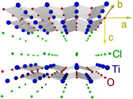
Figure 1: (color online) Crystal structure of TiOCl at room temperature (space group Pnma).

Previously, electron spin resonance (ESR) data suggested that there might be significant changes in the splittings of the $d$-orbitals between $T_{\textrm{c2}}$ and room temperature, based on the temperature dependence of the anisotropic $g$-values.Kataev03 In contrast, significant orbital fluctuations have been discarded by optical spectroscopy studies Rueckamp05 and polarization dependent ARPES measurements.Hoinkis05 However, the first excited $d$-level could not be detected by the optical measurements leaving the question of a possible degeneracy of the lowest lying $d$-orbitals unsolved. Using ESR we reinvestigated TiOCl in detail and find almost temperature-independent $g$-values up to room temperature in agreement with the optical and ARPES studies. Moreover, we discuss possible spin relaxation processes in this compound and analyze the temperature and angular dependence of the ESR linewidth in terms of the symmetric anisotropic exchange interaction and the antisymmetric Dzyaloshinsky-Moriya interaction.

II Sample preparation and experimental details

Single crystals of TiOCl were prepared by chemical vapor transport from TiCl₃ and TiO₂.Schaefer58 The samples have been characterized using x-ray diffraction, specific heat, and magnetization measurements. The crystal structure at room temperature was found to be orthorhombic (space group Pnma) with lattice parameters of $a$ = 0.379 nm, $b$ = 0.338 nm and $c$ = 0.803 nm. The magnetic properties were found to be in excellent agreement with published results.Seidel03 ; Hemberger05 The good quality of the crystals has been clearly confirmed by the susceptibility measurements which reveal a hysteresis at the first-order transition at $T_{\textrm{c1}}$ = 67 K which had not been reported previously.Hoinkis05

The ESR experiments have been carried out with a Bruker ELEXSYS E500 CW-spectrometer at X-band frequency ($\nu\approx$ 9.4 GHz) in the temperature range between 4.2 and 500 K with continuous gas-flow cryostats for He (Oxford Instruments) and N₂ (Bruker). ESR detects the power $P$ absorbed by the sample from the transverse magnetic microwave field as a function of the static magnetic field $H$. The signal-to-noise ratio of the spectra is improved by recording the derivative $dP/dH$ using lock-in technique with field modulation. Dielectric measurements were performed at temperatures 300 $<T<$ 500 K over a frequency range 1 Hz $<\nu<$ 1.08 MHz using a Novocontrol $\alpha$-analyzer.

III Experimental Results

ESR spectra obtained for TiOCl in the paramagnetic regime at different temperatures are displayed in Fig. 2. The spectra consist of a broad, exchange-narrowed resonance line, which is well fitted by a single Lorentzian line shape. The intensity of the ESR signal $I_{\rm ESR}$ is proportional to the static susceptibility Abragam70 and, hence, exhibits also the sharp drop at $T_{\textrm{c1}}$ to the non-magnetic state and the kink at $T_{\textrm{c2}}$. For our samples, $I_{ESR}(T)$ is in agreement with the results obtained in Ref. Kataev03, and, therefore, not shown here.

The temperature dependent ESR linewidth $\Delta H$ and the effective $g$-factor are depicted in Figs. 3(a) and 3(b), respectively. As reported previously, both quantities show an anisotropic behavior with the external magnetic field $H$ applied along the three crystallographic axes of the orthorhombic structure.Kataev03 Above $T\simeq 90$ K the linewidth is largest when $H\|a$ while the values for $H\|b$ and $H\|c$ are almost equal. The linewidth increases monotonously for all three directions for $T>T_{\textrm{c2}}$ K, however, a peculiar change from a negative to positive curvature is observed at about 250 K. Below $T\simeq 90$ K there is a crossover of the linewidth data resulting in the broadest spectra for $H\|b$, which is highlighted in Fig. 7. On approaching the first-order transition at $T_{\textrm{c1}}$, the linewidth for all directions drops down to a value of about 50 Oe. This corresponds to the residual signal due to paramagnetic impurities which will not be further discussed. Focusing on the high-temperature behavior above 250 K we find that the anisotropy of the linewidth becomes smaller and vanishes at about 430 K.

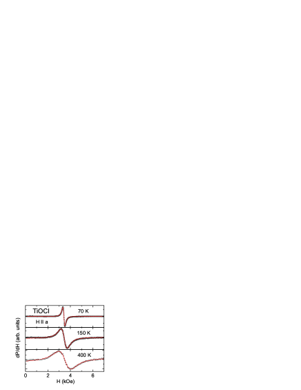
Figure 2: (color online) Temperature evolution of the ESR spectrum in TiOCl for $H\parallel a$. Solid lines represent fits using a Lorentzian line shape.

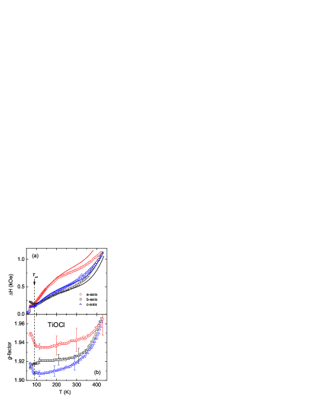
Figure 3: (color online) ESR linewidth (a) and $g$-factor (b) as a function of temperature for the magnetic field applied along the three crystallographic axes. The lines in Fig. 3(a) represent a fit by Eq. (12) using parameters listed in Table 2.

Notably, at the same temperature the anisotropy of the effective $g$-factor vanishes, too (see Fig. 3(b)), and we obtain $g(430~{}\textrm{K})\sim 1.96$ for all three directions. Concomitantly with the change of curvature of the linewidth at 250 K the temperature dependencies of the $g$-factor show a steep increase above 250 K, while the $g$-tensor is nearly constant in the temperature range $T_{\textrm{c2}}<T<250$ K. This behavior differs from previously published results where a much larger and temperature dependent anisotropy of the $g$-factor was reported for $T_{\textrm{c2}}<T<300$ K and interpreted in terms of changes of the energy splittings.Kataev03 Unfortunately, no spectra were shown in Ref. Kataev03, , making it difficult to judge where this discrepancy comes from, especially, because the spectra were fitted with a single Lorentzian line shape in both cases:
Concerning the uncertainty of the obtained $g$-values, one has to take into account the strong increase of the linewidth with temperature, because the uncertainty of the $g$-value becomes larger as the order of magnitude of the linewidth becomes comparable to the resonance field of the ESR spectrum (see e.g. Ref. Deisenhofer02, ; Deisenhofer03, ). Therefore, we assume the uncertainty in the resonance field as 5% of the linewidth and obtain the error bars shown in Fig. 3(b). Despite these error bars our $g$-values at room temperature $g_{a}=1.943$, $g_{b}=1.926$, and $g_{c}=1.919$ differ considerably from the ones presented in Ref. Kataev03, (see Table 1). Here, we would like to emphasize that we investigated several samples, which were shown to be of very high-quality by clearly revealing the hysteresis at $T_{\textrm{c1}}$ in the magnetic susceptibility.Hoinkis05

Table 1: Comparison of the $g$-values at room temperature to experimental results and model calculations of Ref. Kataev03, .

	this work	Ref. Kataev03,	AOM (Model A)	AOM (Model B)
$\textrm{ }g_{a}\textrm{ }$	1.943(12)	2.010	1.946	1.976
$g_{b}$	1.926(8)	1.958	1.935	1.959
$g_{c}$	1.919(8)	1.904	1.926	1.911

Note that the largest discrepancy for the $g$-values is found for $g_{a}$, i.e. with the external field applied along the $a$-axis. Interestingly, for this case there is also a slight deviation in the temperature dependence of $\Delta H_{a}$ in comparison to our data, suggesting that $\Delta H_{a}\simeq\Delta H_{b}$ at room temperature, which we can exclude from our data. Hence, the given error for the $g$-value in Ref. Kataev03, might have been somewhat underestimated. Moreover, none of the calculated sets of $g$-values obtained by using an angular overlap model (AOM) (see Table 1) can reproduce $g_{a}=2.01$ from Ref. Kataev03, , while the corresponding orbital energy levels seem to be in agreement with optical data.Rueckamp05b Instead, the values obtained from the AOM in case of isotropic $\pi$-interaction (model A) describe our $g$-values very nicely. Therefore, we conclude that our $g$-factors correctly reflect the properties of TiOCl and exclude relevant changes in the crystal-field splitting up to room temperature. This is in agreement with direct optical measurements of the $d$-level splittingsRueckamp05 and the fact that x-ray diffraction measurements did not detect significant changes of the crystal structure with temperature.Shaz05

With regard to the increase of the $g$-values towards higher temperatures one has to take into account the larger uncertainty due to the broadening of the line. In principle, however, such a shift could indicate a change of the local structure of the TiO₄Cl₂-octahedra. To decide about this possibility, additional structural investigations for $T>300$ K are desirable.

IV g-factor and crystal field splittings of $\textrm{Ti}^{3+}$

To analyze our experimental $g$-factors, we consider the local environment of the Ti³⁺ ion as a TiO₄Cl₂-octahedron with a strong tetragonal distortion along the $a$-axis. Then we can express the $g$ value parallel ($g_{\|}$) and perpendicular ($g_{\perp}$) to the direction of tetragonal distortion as follows:Abragam70

$$g_{\|}=2-8\lambda_{\parallel}/\Delta_{0},\qquad g_{\perp}=2-2\lambda_{\perp}/\Delta^{\prime}$$ (1)

Here $\lambda_{\parallel}$ ($\lambda_{\perp}$) and $\Delta_{0}$ ($\Delta^{\prime}$) denote the spin-orbit (SO) coupling parameter and the relevant crystal-field splitting, respectively, for the magnetic field applied parallel (perpendicular) to the $a$-axis. Recalling the above discussion about the increase of uncertainty in the $g$-values with increasing temperatures (see Fig. 3(b)), we will restrict the following evaluation to the $g$-values $g_{a}=1.935(8)$, $g_{b}=1.921(5)$, and $g_{c}=1.908(5)$ obtained at 150 K, because this temperature is well above $T_{\textrm{c1}}$ and the uncertainty is still quite low. Note, however, that the absence of any significant temperature dependence of the $g$-factor up to room temperature allows to apply the following results in this temperature range with good accuracy.

Thus, identifying the experimental value of $g_{a}$ with $g_{\|}=1.935(10)$ and substituting $\lambda_{\parallel}$ by the isotropic free-ion value $\lambda_{\textrm{fi}}/k_{B}=224$ K for Ti³⁺,Abragam70 we derive the energy splitting between the ground state and the $|d_{x^{2}-y^{2}}\rangle$ level to be $\Delta_{0}=\Delta_{x^{2}-y^{2}}\approx 2.4(2)$ eV.LocalCoord In comparison to the value $\Delta_{x^{2}-y^{2}}^{\textrm{(opt)}}=1.5$ eV obtained by optical measurementsRueckamp05 the value derived from our $g$-factor is too large. Therefore, we have to take into account a covalence reduction of the spin-orbit coupling $\lambda_{\parallel}$.Abragam70 To estimate the reduction factor we use the experimental value $\Delta_{x^{2}-y^{2}}^{\textrm{(opt)}}$ and obtain $\lambda_{\parallel}/k_{B}\simeq 140$ K for TiOCl, considerably smaller than the free-ion value $\lambda_{\textrm{fi}}$ but in agreement with literature.Abragam70 ; Kataev03 This large splitting allows to discard the scenario of $|d_{x^{2}-y^{2}}\rangle$ being the first excited state approximately $0.34$ eV above the ground state (point-charge model), in favor of cluster calculations predicting the first excited state to be $(|d_{xz}\rangle-|d_{yz}\rangle)/\sqrt{2}$.Kataev03 ; Rueckamp05

Additionally, the $g$-factors in the $(bc)$-plane can be used to estimate the energy of the first exited state in TiOCl. In order to simulate the anisotropy of the $g$-factor with the AOM model (see Table 1), also Kataev and coworkers had to consider covalence reduction factors, which were chosen to be anisotropic because of a presumably stronger covalency of the short Ti-O bond along the $a$-axis compared with the longer bonds in the ($bc$)-plane. We cannot unambiguously determine the covalence reduction within the $(bc)$-plane, but we can use $\lambda_{\perp}=140$ K and the free ion value $\lambda_{\textrm{fi}}=224$ K to obtain lower and upper limits for the energy splittings. Starting with $\lambda_{\perp}\equiv\lambda_{\parallel}=140$ K and $g_{\perp}=(g_{b}+g_{c})/2\approx 1.92(1)$ we derive $\Delta^{\prime}_{\lambda_{\parallel}}\approx 0.3$ eV for the energy splitting of the doublet $|d_{xz}\rangle$, $|d_{yz}\rangle$ with respect to the ground state. In the real structure this doublet splits into the lower antisymmetric $(|d_{xz}\rangle-|d_{yz}\rangle)/\sqrt{2}\equiv|-\rangle$ (energy $\Delta_{1}$) and higher symmetric $(|d_{xz}\rangle+|d_{yz}\rangle)/\sqrt{2}\equiv|+\rangle$ (energy $\Delta_{2}$) state. Using $2/\Delta^{\prime}=1/\Delta_{1}+1/\Delta_{2}$ and the experimental value $\Delta_{2}=0.65(\pm 0.15)$ eV,Rueckamp05 we finally obtain the lower limit $\Delta_{1}^{(\lambda_{\parallel})}=0.2(1)$ eV. Analogously, we derive the upper limit $\Delta_{1}^{(\lambda_{\textrm{fi}})}=0.4(1)$ eV, narrowing down the energy of the first exited state to $\Delta_{1}=0.2-0.4$ eV. This is in good agreement with the theoretical estimates of $\Delta_{1}=0.25-0.3$ eV obtained by cluster calculations.Rueckamp05

Thus, by means of ESR we can exclude the degeneracy of the first and second excited states in TiOCl, as indicated by band-structure results,Seidel03 ; Saha-Dasgupta04 corroborating the results obtained by optics and ARPES measurements.Rueckamp05 ; Hoinkis05

V Spin relaxation in TiOCl

V.1 General remarks

Having identified the character and splitting of the ground and low lying excited states via the $g$-factors, we will now discuss the angular and temperature dependence of the linewidth above $T_{\textrm{c1}}$, which provides information on the microscopic spin dynamics involving these energy levels. The behavior of the ESR linewidth in TiOCl can be clearly divided into the three regimes $T<90$ K, 90 K $<T<250$ K, and $T>250$ K. In the temperature range $T_{\textrm{c1}}<T<90$ K the linewidth is almost constant (for $H\|a,c$) or decreases (for $H\|b$) on increasing temperature. This behavior changes at about 90 K together with a change of the linewidth anisotropy (see Fig. 7) to the monotonous increase for all directions. At high temperatures $T>250$ K a strong additional increase of $\Delta H(T)$ dominates this saturation behavior (see Fig. 6) and the anisotropy of the line vanishes (Fig. 3). We attribute these different regimes to the competition of relaxation mechanisms prevailing at different temperatures, which will be discussed in detail in the following. At first we have to single out the relevant interactions which drive the relaxation in TiOCl:

Single-ion anisotropy is absent for Ti³⁺ (S=$1/2$). Other sources of line broadening such as dipolar interaction or hyperfine coupling are negligible as a result of the large isotropic exchange $J/k_{\rm B}=660$ K. Taking into account the average distance between the Ti-ionsShaz05 of about 3.355 Å and the value of the hyperfine constant $A_{\textrm{Ti}^{3+}}=6\cdot 10^{-4}$ cm^-1 (see Ref. Altshuler64, ) we can estimate the contribution to the linewidth from these sources as $10^{-1}$ Oe and $10^{-5}$ Oe, respectively. The minor importance of these interactions for the linewidth broadening in low-dimensional systems with a strong exchange coupling has been discussed in detail e.g. by Pilawa et al. Pilawa97 for CuGeO₃ and Yamada et al. Yamada98 for NaV₂O₅. A larger contribution to the ESR linewidth could be expected for the anisotropic Zeeman interaction in case of different Ti³⁺ sites in adjacent layers.Pilawa97 However, this broadening strongly depends on the value of the resonance field $H_{\textrm{res}}$. At X-band frequency used in our experiment ($H_{\textrm{res}}\sim 3$ kOe) the resulting contribution is less than 1 Oe for any reasonable choice of parameters (e.g. an interlayer coupling $J_{\textrm{inter}}\approx 0.05\cdot J$ (Ref. Saha-Dasgupta04, ) and $\Delta g\sim 0.3$).

The remaining relevant contributions stem from the anisotropic exchange interactions. Conventional estimationsMoriya60 of their magnitude result in values at least two order of magnitudes higher as for the other sources of line broadening. Note, however, that the applicability of such estimations for low-dimensional systems like TiOCl has been questioned, recently.vonNidda02 ; Oshikawa02 ; Choukroun01 Hence, one has to analyze carefully each spin system under consideration on a microscopic level.

In general, anisotropic exchange interactions arise due to virtual hopping processes of electrons or holes between two interacting ions via the bridging diamagnetic ions in combination with the SO coupling ${\cal H}_{\textrm{SO}}=\lambda L_{\alpha}S_{\alpha}$. Here $L_{\alpha}$ and $S_{\alpha}$ denote the orbital and spin momentum of the magnetic ion, respectively. For a more detailed discussion of the exchange interactions we refer to Refs. Bencini90, and Eremin85, . Now, we will discuss the symmetric part of the anisotropic exchange (AE) interaction as well as the antisymmetric Dzyaloshinsky-Moriya (DM) exchange interaction and their importance for the spin relaxation in TiOCl. Their influence on the spin relaxation will be analyzed in terms of the so called moment method: In the case of sufficiently strong exchange interaction the ESR linewidth can be obtained from the second moment

$$M_{2}=h^{2}\langle(\nu-\nu_{0})^{2}\rangle=-\frac{\langle[{\cal H}_{\textrm{int}},S^{+}]\,[{\cal H}_{\textrm{int}},S^{-}]\rangle}{\langle[S^{+},S^{-}]\rangle}$$ (2)

of the ESR line via the relationKubo54

$$\Delta H=\frac{1}{g\mu_{\textrm{B}}}\cdot\frac{M_{2}}{J},$$ (3)

where $\mu_{\textrm{B}}$ denotes the Bohr magneton. This method is well established only in the high-temperature limit $T>J/k_{\textrm{B}}$. In this limit the second moment is temperature independent and can be expressed via the parameters of the microscopic spin Hamiltonian ${\cal H}_{\textrm{int}}$.Kochelaev03 As the exchange constant is quite large in TiOCl, we do not reach the high-temperature limit in our experiment. However, the anisotropy of the linewidth yields the relative values of the exchange parameters even at low temperatures.Oshikawa02 In the following we determine the leading components of the symmetric AE tensor and of the DM vector. Inserting these parameters into Eq. (2) yields the angular dependence of the linewidth which then can be compared to the experimental observations.

V.2 Symmetric anisotropic exchange

The importance of symmetric anisotropic exchange for low-dimensional systems has been emphasized in a recent study by Eremin and coworkers for $\alpha^{\prime}$-NaV₂O₅.Eremin05 It was shown that it is necessary to take into account both the exchange geometry and the energies of the involved orbital states in order to obtain reliable estimates of the AE on a microscopic basis. All electron transfers processes both between the exited states on two sites and between the exited and ground states of the involved ions must be considered. Then, contributions of possible pathways to the AE can be calculated using the respective values of hopping integrals and energy splittings.Eremin05 Such microscopic estimations are beyond the scope of this paper, but we will discuss qualitatively the relevant exchange processes in TiOCl based on the analysis of Ref. Eremin05, .

Crystal-field field splittings of the relevant exited states have been already estimated above (see Sec. IV) and in order to illustrate the exchange geometry via these orbital levels we show the charge-distribution pictures for the pathways of AE for the intra-chain and inter-layer exchange in Figs. 4(a) and 4(b), respectively. The inter-chain AE within one layer is not effective here because of the orthogonality of the ground-state orbital with respect to the direction of the exchange.

In analogy to the estimations made in Ref. Eremin05, we argue that the pathways of AE shown in Fig. 4 are by far the most relevant ones. The first exchange process between neighboring Ti ions in the chain (depicted at the left side of the upper panel) with an electron transfer between $|d_{x^{2}-y^{2}}\rangle$ and $|d_{xy}\rangle$-orbitals becomes important as a result of the strong $\sigma$-bounding between the titanium $d$– and the oxygen $p$-orbitals. The importance of the second intra-chain AE process (at the right side of the upper panel of Fig. 4) via $|-\rangle$-orbitals is due to the small energy $\Delta_{1}$ of the involved exited state. Note that only the exchange paths between the exited $|-\rangle$-states are shown in the second case, since the exchange path between the ground $|d_{xy}\rangle$-orbitals has already been discussed elsewhere.Seidel03 In the lower panel of Fig. 4 the dominating exchange paths of the inter-layer AE are presented: the left one being between $|-\rangle$ and $|d_{xy}\rangle$-orbitals and the second between $|+\rangle$ and $|d_{xy}\rangle$-orbitals. These processes are of the same order of magnitude as the intra-chain exchange and cannot be neglected.

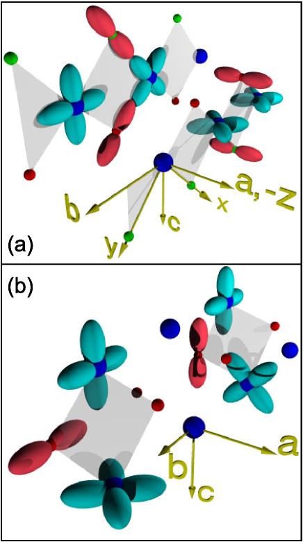
Figure 4: (color online) Schematic pathway of the symmetric anisotropic exchange between Ti ions in TiOCl. Big spheres denote Ti ions, small spheres – O and Cl ions. Upper frame: The most relevant intra-chain ($\parallel b$-axis) exchange paths. Left one – between the ground state $|d_{xy}\rangle$-orbital on one site and the exited $|d_{x^{2}-y^{2}}\rangle$-orbital on the other site, second one – between two exited $|-\rangle$-orbitals on both sites. Lower frame: two dominating exchange paths of the inter-chain AE between a Ti ion in the $|d_{xy}\rangle$-state and the nearest-neighbor Ti ion from the adjacent chain in the exited states $|-\rangle$ (left) or $|+\rangle$ (right) .

The non-zero elements of the exchange tensors can be determined via the SO operators included in this process.Bencini90 ; Yosida96 ; Eremin85 For the first intra-chain AE process (via the $|d_{x^{2}-y^{2}}\rangle$-orbital) the exited state is connected to the ground state $d_{xy}$ of the same Ti ion via SO coupling with only one nonzero matrix element, namely $\langle d_{x^{2}-y^{2}}|L_{z}|d_{xy}\rangle=-2i$. Following Ref. Eremin05, , all AE processes via this level contribute to $J_{zz}$ only. Taking now into account the relation for the diagonal components of the AE tensor $\sum J_{\alpha\alpha}=0$ we obtain for this process

$$J_{zz}^{(|x^{2}-y^{2}\rangle)}=-2J_{xx}^{(|x^{2}-y^{2}\rangle)}=-2J_{yy}^{(|x^{2}-y^{2}\rangle)}.$$ (4)

All other AE processes which make a considerable contribution to the linewidth in TiOCl involve the $|-\rangle$ or $|+\rangle$-orbitals ($|\pm\rangle\equiv\{|d_{xz}\rangle\pm|d_{yz}\rangle\}/\sqrt{2}$), which are connected to the ground state orbital $|d_{xy}\rangle$ via the matrix elements $\langle d_{xz}|L_{x}|d_{xy}\rangle=i$ and $\langle d_{yz}|L_{y}|d_{xy}\rangle=-i$. The resulting nonzero elements $J_{xx}$ and $J_{yy}$ of the AE tensor have the same magnitude because of symmetry reasons and they have the same sign, because the expression for $J_{\alpha\beta}$ (see Ref. Eremin05, ) depends on the square of the orbital momentum. Thus, we can write the AE tensor for these processes as $J_{zz}^{(|-\rangle,|+\rangle)}=-2J_{xx}^{(|-\rangle,|+\rangle)}=-2J_{yy}^{(|-\rangle,|+\rangle)}$. It becomes clear that the maximal component of the anisotropic exchange tensor is $J_{zz}$. Therefore, we would expect the maximal linewidth for $H\|z$ in agreement with the experimental data for $T>90$ K.

Consequently, we can describe the resulting angular dependence of $\Delta H$ in terms of the moment method in analogy to CuGeO₃ (Ref. Eremina03, )

$$\Delta H_{AE}(T,\theta)=K_{AE}(T)(1+\textrm{cos}^{2}\theta),$$ (5)

where $\theta$ is the polar angle of $H$ with respect to the $a\equiv-z$ axis and $K_{AE}(T)$ is proportional to the strength of the AE interaction. This parametrization does not allow to obtain the exact values of the anisotropic exchange parameters, but it is valid for all temperatures and, hence, we will apply it to describe our data using $K_{AE}$ as a fit parameter.

Concerning the temperature dependence of the ESR linewidth produced by AE exchange interaction, clear theoretical predictions do only exist in two limiting cases: (i) For the high-temperature regime $T>J$, the linewidth approaches the result of the Kubo-Tomita theoryKubo54 $\Delta H^{(T>J)}_{AE}(T)\rightarrow K_{AE}(\infty)\propto J_{\alpha\beta}^{2}/J=\textrm{const}$, and (ii) the result $\Delta H^{(T\ll J)}_{AE}(T)\propto(K_{AE}(\infty)/J)\cdot T$ in the case $T\ll J$ for the $S=1/2$ quantum antiferromagnetic chain.Oshikawa02 To model the crossover regime we will use the following empirical expression which has already provided a successful description for several low-dimensional systems like CuGeO₃,Eremina03 LiCuVO₄,vonNidda02 and Na_1/3V₂O₅ (Ref. Heinrich04, ):

$$\Delta H_{AE}(T)\equiv K_{AE}(T)=K_{AE}(\infty)\cdot\textrm{e}^{-\frac{C_{1}}{T+C_{2}}}.$$ (6)

Thus, the fit parameters to describe the contribution of the AE are $K_{AE}(\infty),C_{1},C_{2}$.

V.3 Dzyaloshinsky-Moriya interaction

The contribution of the DM interaction to the ESR line broadening in one-dimensional systems is a heavily debated topic at the moment.Yamada98 ; Choukroun01 ; Oshikawa02 ; Ivanshin03 Using the well-established high-temperature Kubo-Tomita approach,Kubo54 the DM interaction was considered to be the dominating relaxation mechanism in spin-chain compounds like e.g. NaV₂O₅.Yamada98 However, the applicability of this approach was questioned in a field theoretical one by Oshikawa and Affleck,Oshikawa02 arguing that the contribution of the DM interactions is strongly overestimated by the Kubo-Tomito approach. A recent conclusive experimental conformation of the results of Oshikawa and Affleck was reported by Zvyagin et al. , who unambiguously showed that the importance of the DM interaction in antiferromagnetic spin-1/2 chains has to be considered with special care.Zvyagin05 While the DM interaction was not explicitly discussed by Kataev and coworkers for TiOCl,Kataev03 Kato et al. considered it to be the main source of line broadening in the isostructural system TiOBr by referring to the Kubo-Tomita approach.Kato05

In general, the structure of TiOCl allows for a contribution of the antisymmetric DM interaction

$${\cal H}_{DM}^{(ij)}=\mathbf{d}_{ij}\cdot[\mathbf{S}_{i}\times\mathbf{S}_{j}]$$ (7)

between the Ti spins $\mathbf{S}_{i}$ and $\mathbf{S}_{j}$ via an intermediate diamagnetic ion.Dzialoshinski58 ; Moriya60 The DM vector $\mathbf{d}_{ij}$ is an axial vector perpendicular to the plane spanned by the Ti spins and the ligand ion, determined by $\mathbf{d}_{ij}=d^{(l)}\cdot[\mathbf{n}_{il}\times\mathbf{n}_{jl}]$, where the unit vectors $\mathbf{n}_{il}$ and $\mathbf{n}_{jl}$ connect the spins $i$ and $j$ with the bridging ion $l$, respectively.Keffer62 When the point bisecting the straight line connected two interacting ions is not a center of inversion, which is the case for TiOCl or TiOBr,Shaz05 one can expect that $\mathbf{d}_{ij}\neq 0$.Moriya60 Kato et al. Kato05 argued that the maximal component of the DM vector in TiOBr is parallel to the $a$ axis, accounting for the maximal linewidth along the $a$ axis in the temperature regime $T_{\textrm{c1}}<T<T_{\textrm{c2}}$. Note, that in TiOCl the maximum linewidth in this temperature regime is observed for $H\parallel b$ (Fig. 7 and Ref. Kataev03, ).

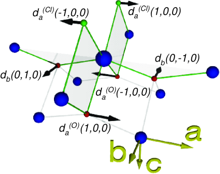
Figure 5: (color online) Next-neighbor bonds of the Ti ion together with the associated parameters of the antisymmetric anisotropic exchange. $d_{b}$, $d_{a}^{(\textrm{O})}$ and $d_{a}^{(\textrm{Cl})}$ denote the Dzyaloshinsky-Moriya parameters for the exchange along the $a$-axis, along the $b$-axis via the oxygen ion and along the $b$-axis via the chlorine ion, respectively. Components of the DM vectors are given in the depicted cartesian coordinate system {$b$,$c$,$a$}. Big spheres denote Ti ions, small spheres – O and Cl ions.

In what follows, we will analyze the DM interaction in TiOCl considering every next-neighbor bond of the Ti ion on basis of the structural data of Shaz et al. at room temperature.Shaz05 All bonds of the Ti ion together with the corresponding DM vectors are shown in Fig. 5. Only interactions of Ti ions in the same layer give rise to the antisymmetric exchange in TiOCl because of the existence of an inversion center between the Ti ions from adjacent layers. The two remaining contributions arise from the chains of the Ti ions along the $b$ and $a$ directions. The first one, which results in a component of $\mathbf{d}_{ij}$ in the $a$ direction, has been considered in Ref. Kato05, as the dominating source of the line broadening. However, we would like to point out that there are two different bridging ions (Cl^- and O^2-) leading to DM vectors with opposite sign in this case. Although the two paths are asymmetric ($n_{\textrm{Ti-Cl}}\simeq 2.393$ Å, $n_{\textrm{Ti-O}}\simeq 2.187$ Å at T = 295 K)Shaz05 and, hence, lack inversion symmetry, one can assume that the opposite DM vectors will partially compensate each other. If we denote the respective DM parameters $d^{(l)}$ as $d_{a}^{(\textrm{O})}$ and $d_{a}^{(\textrm{Cl})}$ for the exchange via the O^2- and Cl^- ions, respectively, only its difference $\Delta d_{a}=d_{a}^{(\textrm{O})}-d_{a}^{(\textrm{Cl})}$ will give rise to the ESR line broadening and can be detected experimentally (see e.g. the discussion about the cancelation of DM interaction in LiCuVO₄)vonNidda02 . Looking now at the contribution of the inter-chain DM interaction (between two neighboring Ti³⁺ sites along the $a$ axis via the oxygen ion lying in the same $(ac)$-plane), we can conclude that the corresponding DM vector is pointed along the $b$-axis (see Fig. 5).

The general expression for the $M_{2}$ due to the DM interaction has been given in Ref. Deisenhofer02, . In the case of TiOCl only two intra-chain and two inter-chain contribution must be taken into account by the calculation of the respective ESR line broadening. Estimation of the ”geometrical factors” $\textbf{G}^{(l)}=[\mathbf{n}_{il}\times\mathbf{n}_{jl}]$ yields: (i) for the inter-chain exchange $G_{b}^{(\textrm{O})}=\pm 0.501\approx 1/2$, (ii) $G_{a}^{(\textrm{O})}=\pm 0.98\approx 1$ and $G_{a}^{(\textrm{Cl})}=\pm 0.99\approx 1$ for the intra-chain exchange via the O^2- and Cl^- ions, respectively. Therefore, we obtain the following expression for the second moment of the DM interaction in the crystallographic system:

$$\begin{array}[]{ll}M_{2}^{DM}(\theta,\varphi)\propto&(d_{b}\cdot 1/2)(1+\textrm{sin}^{2}\theta\textrm{cos}^{2}\varphi)+\\ &+(\Delta d_{a}\cdot 1)(1+\textrm{cos}^{2}\theta),\end{array}$$ (8)

where $\theta$ and $\varphi$ are the polar and azimuthal angles of $H$ with respect to the $a$ axis. Finally, the ratios of the linewidth along the three crystallographic axes read

$$\begin{array}[]{ll}\Delta H_{b}:\Delta H_{a}:\Delta H_{c}&=M_{2}(\frac{\pi}{2},0):M_{2}(0,\varphi):M_{2}(\frac{\pi}{2},\frac{\pi}{2})\\ &=\frac{2+(2\Delta d_{a}/d_{b})^{2}}{1+(2\Delta d_{a}/d_{b})^{2}}:\frac{1+2(2\Delta d_{a}/d_{b})^{2}}{1+(2\Delta d_{a}/d_{b})^{2}}:1.\end{array}$$ (9)

Simplifying this expression for the case $\Delta d_{a}/d_{b}\rightarrow 0$, one gets $\Delta H_{b}:\Delta H_{a}:\Delta H_{c}=2:1:1$ and the angular dependence

$$\Delta H_{DM}^{(\Delta d_{a}/d_{b}\rightarrow 0)}(T,\theta,\varphi)=K_{DM}(T)(1+\textrm{sin}^{2}\theta\textrm{cos}^{2}\varphi),$$ (10)

where $\varphi$ is the azimuthal angle of $H$ in $(bc)$-plane with respect to the $b$ axis and $K_{DM}(T)$ is proportional to the strength of the DM interaction.

Regarding the temperature dependence of $\Delta H_{DM}$ (or $K_{DM}(T)$), we will use the result obtained by Oshikawa and Affleck $\Delta H^{(T\ll J)}_{DM}(T)\propto J^{2}/T^{2}$ obtained for the case of a staggered DM interaction ${\cal H}_{DM}^{(ij)}=\sum_{i}\textbf{d}_{i}\cdot[\textbf{S}_{i}\times\textbf{S}_{i+1}]$ with $\textbf{d}_{i}=(-1)^{i}\textbf{d}$ for $T\ll J$.Oshikawa02 Assuming that this temperature dependence also holds for a uniform DM interaction along the chain as in our case, we will apply the power law

$$\Delta H_{DM}(T)\equiv K_{DM}(T)=K_{DM}(\infty)\left(\frac{J}{T}\right)^{2}$$ (11)

to fit the experimental data using $K_{DM}(\infty)$ as a fit parameter. An analytical expression for the crossover behavior from this power-law (valid for $T\ll J=660$ K) to the constant high-temperature value of the Kubo-Tomita approach has not been derived up to now. Therefore, we extrapolate the power law up to $T=J$ and identify $K_{DM}(T=J)=K_{DM}(\infty)$ in order to compare the experimental values to the theoretical estimates of the Kubo-Tomita approach. We would like to recall that the ratio of $\Delta H$ along different axes in Eq. (9) evaluated in the high-temperature limit does not depend on the form of the temperature dependence.

VI Analysis and Discussion of the ESR linewidth

Starting out with the superposition of the angular and temperature dependence for the AE and DM interactions, it is possible to describe the anisotropy and the temperature dependence of the linewidth for $T_{\textrm{c1}}<T<250$ K, but the change of curvature (Fig. 3) for $T>250$ K clearly shows that an additional relaxation channel dominates at higher temperatures. Before we discuss the low-temperature data in detail, we shortly comment on possible reasons for this high-temperature behavior.

In order to determine the temperature dependence more accurately up to 500 K, we additionally performed measurements of crushed single crystals (see Fig. 6). This was necessary because of the fact that the single crystals of TiOCl are thin platelets of small mass and that the linewidth above room temperature is already very large.

It turns out that the strong increase of the ESR linewidth with temperature can be very well accounted for by adding an exponential term $K_{\textrm{exp}}\cdot e^{-\Delta_{ESR}/k_{\textrm{B}}T}$ to the temperature dependence of the anisotropic exchange interactions:

$$\begin{array}[]{ll}\Delta H(T)=&K_{DM}(\infty)\cdot\left(\frac{J}{T}\right)^{2}+\\ &+K_{AE}(\infty)\cdot\textrm{e}^{-\frac{C_{1}}{T+C_{2}}}+\\ &+K_{\textrm{exp}}\cdot e^{-\Delta_{ESR}/k_{\textrm{B}}T}.\end{array}$$ (12)

The resulting fit is shown as a solid line in Fig. 6, yielding $\Delta_{ESR}=0.28$ eV. The exponential nature of the additional increase is highlighted in the inset of Fig. 6, where the reduced linewidth data $\Delta H_{\textrm{red}}$ are plotted after subtraction of the contributions of the AE and DM interactions (dashed line in Fig. 6).

An additional relaxation channel via thermally activated charge carriers might cause an exponential increase of $\Delta H(T)$, as it has been discussed for doped manganites,Shengelaya00 and at the metal-to-insulator transition in $\beta$-Na_1/3V₂O₅.Heinrich04 In both cases the leading contribution to the temperature dependence is determined by the Arrhenius law of the conductivity $e^{-\Delta_{\sigma}/2k_{\textrm{B}}T}$. The corresponding temperature behavior of the dc-conductivity which could be obtained from dielectric measurements.Lunkenheimer02 In an Arrhenius representation one can extract an activation energy $\Delta_{\sigma}/2\approx 0.31$ eV (see inset of Fig. 6).Lunkenheimerunpublished Although this value is similar to the one obtained from the ESR linewidth, it is by far too small compared with the experimental gap value of about 2 eV observed by optical spectroscopy.Rueckamp05b Therefore, such a scenario appears rather unlikely. Alternatively, the exponential increase can be interpreted analogously to the case of the one-dimensional magnet CuSb₂O₆. In this compound a similar temperature dependence of the linewidth with $\Delta_{ESR}^{\textrm{(CuSb}_{2}\textrm{O}_{6})}=0.13$ eV was observed and explained in terms of a thermally activated dynamic Jahn-Teller (JT) process.Heinrich03 However, a rigorous theoretical treatment of this effect has not yet been undertaken. Moreover, we would like to mention that the obtained value $\Delta_{ESR}=0.28$ eV is very close to the energy 0.3(1) eV of the first excited state. This might indicate the involvement of exited orbital states in this relaxation process. To finally decide about the origin of the high-temperature relaxation, however, detailed structural studies in this temperature region are necessary.

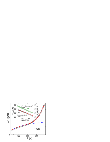
Figure 6: (color online) Temperature dependence of the ESR linewidth for a powder sample together with a fit by Eq. (12). The obtained fit parameters are given in Table 2. $\Delta H_{\textrm{ex}}(T)=\Delta H_{AE}(T)+\Delta H_{DM}(T)$ is shown as dashed line. Inset: reduced contribution $\Delta H_{\textrm{red}}(T)=\Delta H(T)-\Delta H_{\textrm{ex}}(T)$ compared to conductivity as Arrhenius plot.

Fixing the value $\Delta_{ESR}=0.28$ eV, we now proceed to describe the anisotropic temperature dependence of the linewidth for the main orientations of the single crystal. Note that $\Delta_{ESR}$ should not depend on the orientation of the magnetic field with respect to the crystal axes, justifying the further use of this value for the single crystal. The resulting fit curves are shown in Fig. 3 and the obtained fit parameters are given in Table 2. The agreement between fit and data below 250 K is excellent (see also Fig. 7), but at higher temperatures deviations are clearly visible for $H\|\,a$ and $H\|\,b$. The anisotropy inferred from the AE and the DM interaction below 250 K is somewhat larger than the observed one. The gradual suppression of the anisotropy with increasing temperature may result from the thermal occupation of higher lying $d$-levels, which is also in agreement with the disappearance of the anisotropy of the $g$-tensor (Fig. 3). A similar effect was observed at the transition from a cooperative static JT-effect to a dynamic JT-phase in (La:Sr)MnO₃.Kochelaev03

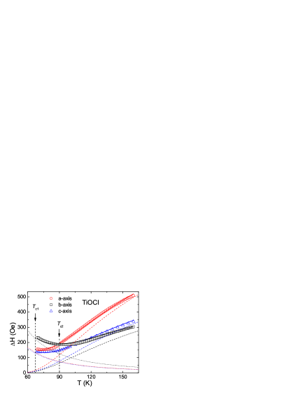
Figure 7: (color online) Temperature dependence of the ESR linewidth in TiOCl for the magnetic field applied parellel to the three crystallographic axes. The fit curves were obtained by the sum of $\Delta H_{AE}(T)$ and $\Delta H_{DM}(T)$ (Eqs. (6),(11)) with the parameters listed in Table 2. The dashed and dotted lines represent the contributions from the AE and DM interactions, respectively.

Table 2: Parameters determined from fits on the temperature (Figs. 3,6,7) and angular (Fig. 8) dependencies of the linewidth by the Eq. (12) and (13), respectively. The parameters $C_{1}=129.12$ K, $C_{2}=-38.1$ K, $\Delta_{ESR}=0.28$ eV, $K_{\textrm{exp}}=0.87$ MOe are assumed to be isotropic. Parameter $S_{AE}$ used by the fit of the angular dependence of $\Delta H$ in the $(ab)$-plane is equal to 1.05.

	$K_{AE}(\infty)\textrm{ [Oe]}$	$K_{DM}(\infty)\textrm{ [Oe]}$
$H\|\,a$ (single crystal)	$1429$	$1.397$
$H\|\,b$ (single crystal)	$765$	$2.319$
$H\|\,c$ (single crystal)	$930$	$1.344$
crushed single crystal	$990$	$1.344$

Let us turn to the discussion of the anisotropic exchange contributions which dominate the relaxation below 250 K. Using the obtained fit parameters we additionally fitted the angular dependence of the linewidth data for the single crystal in the crystallographic $(ab)$-plane (Fig. 8) by using

$$\begin{array}[]{lll}\Delta H^{(ab)}(T,\theta)&=&K_{DM}^{(H\|\,a)}(\infty)\cdot\left(\frac{J}{T}\right)^{2}(1+\textrm{sin}^{2}\theta)+\\ &+&\frac{1}{S_{AE}}\cdot K_{AE}^{(H\|\,b)}(\infty)\cdot\textrm{e}^{-\frac{C_{1}}{T+C_{2}}}(1+\textrm{cos}^{2}\theta)+\\ &+&K_{\textrm{exp}}\cdot e^{-\Delta_{ESR}/k_{\textrm{B}}T},\end{array}$$ (13)

where $\theta$ denotes the angle in the $(ab)$-plane with respect to the $a$ axis. Here, we took into account only the DM contribution along the crystallographic $b$-axis (see Sec. V.3). Concerning the AE interaction, we had to introduce the additional fit parameter $S_{AE}\approx K_{AE}^{(H\|\,a)}(\infty)/[2\cdot K_{AE}^{(H\|\,b)}(\infty)]=1.05$ which indicates the deviation from the theoretically expected ratio of 1, if only the AE paths described above are taken into account (i.e. $J_{zz}=-2J_{xx}=-2J_{yy}$). The fact that $S_{AE}=1.05$ can be explained by small contributions of the other relaxation processes (see Sec. V.1). Thus, we were able to corroborate the validity of the fit parameters given in Table 2 by a consistent description of the temperature and angular dependence of the linewidth. Moreover, we find a good agreement of the ratios of the obtained high-temperature fit parameters for the DM interactions $K_{DM}^{(H\|\,b)}(\infty):K_{DM}^{(H\|\,a)}(\infty):K_{DM}^{(H\|\,c)}(\infty)\equiv\Delta H_{b}^{\textrm{(fit)}}:\Delta H_{a}^{\textrm{(fit)}}:\Delta H_{c}^{\textrm{(fit)}}=1.72:1.04:1$ with the theoretically expected ratio $2:1:1$.

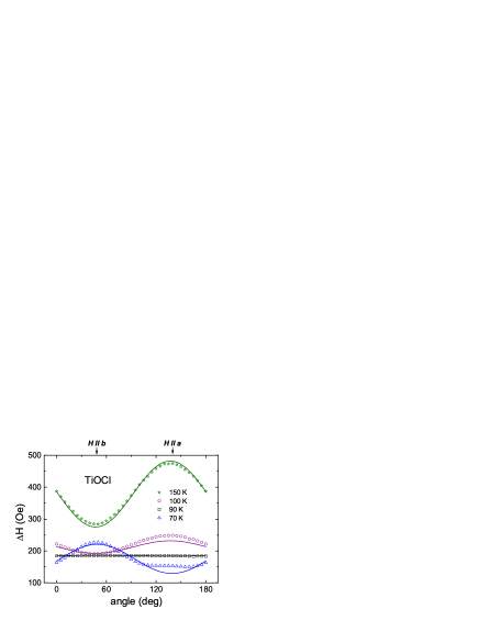
Figure 8: (color online) Angular dependence of the ESR linewidth $\Delta H$ in TiOCl for the magnetic field applied within the ($ab$)-plane at different temperatures between 70 and 150 K. The solid lines represent the fit by the Eq. (13), where the fitting parameters are taken from Table 2.

Looking at the corresponding contributions of AE and the DM interactions shown in Fig. 7, it becomes clear that the dominant relaxation mechanism for $T>90$ K is the AE, while the DM interaction takes over for $T_{\textrm{c1}}<T<90$ K. This competition is nicely evidenced by the corresponding orientation dependences and the crossover at about 90 K (Fig. 8). However, significant contributions of the DM interactions can already be anticipated below 135 K where the linewidth for $H\parallel b$ already becomes larger than the one for $H\parallel c$. Here, we have to emphasize that our analysis of the DM interaction is based on the room-temperature structure and does not take into account a possible structural phase transition at $T_{\textrm{c2}}$. Since the linewidth data does not reveal a discontinuity at $T_{\textrm{c2}}$ but a smooth crossover, we conclude that the structural changes do not significantly alter the involved relaxation processes.

VII Summary

In summary, we have investigated the temperature dependence ($T<500$ K) of the ESR linewidth $\Delta H$ and the $g$ value in TiOCl. From the $g$ values we derive the energy of the first excited state as $\Delta_{1}=0.2-0.4$ eV, in good agreement with theoretical estimations. Furthermore, we describe the angular and temperature dependence of the linewidth as a competition of the anisotropic exchange interactions and an additional exponential increase for $T>250$ K higher temperature that might be related to thermally activated lattice fluctuations. We could show that the line broadening is dominated by the symmetric anisotropic exchange for 90 K $<T<250$ K which produces the maximal linewidth along the $a$ direction, while the antisymmetric DM interaction leads to the crossover at about 90 K with the maximal linewidth along the $b$ direction.

- (1) B. Keimer, D. Casa, A. Ivanov, J. W. Lynn, M. v. Zimmermann, J. P. Hill, D. Gibbs, Y. Taguchi, and Y. Tokura, Phys. Rev. Lett. 85, 3946 (2000).
- (2) M. Cwik, T. Lorenz, J. Baier, R. Muller, G. Andre, F. Bouree, F. Lichtenberg, A. Freimuth, R. Schmitz, E. Muller-Hartmann, and M. Braden, Phys. Rev. B 68, 060401 (2003).
- (3) J. Hemberger, H.-A. Krug von Nidda, V. Fritsch, J. Deisenhofer, S. Lobina, T. Rudolf, P. Lunkenheimer, F. Lichtenberg, A. Loidl, D. Bruns, and B. Buchner, Phys. Rev. Lett. 91, 066403 (2003).
- (4) R. M. Eremina, M. V. Eremin, V. V. Iglamov, J. Hemberger, H.-A. Krug von Nidda, F. Lichtenberg, and A. Loidl, Phys. Rev. B 70, 224428 (2004).
- (5) C. Ulrich, G. Khaliullin, S. Okamoto, M. Reehuis, A. Ivanov, H. He, Y. Taguchi, Y. Tokura, and B. Keimer, Phys. Rev. Lett. 89, 167202 (2002).
- (6) A. Seidel, C. A. Marianetti, F. C. Chou, G. Ceder, and P. A. Lee, Phys. Rev. B 67, 020405(R) (2003).
- (7) M. Shaz, S. van Smaalen, L. Palatinus, M. Hoinkis, M. Klemm, S. Horn, and R. Claessen, Phys. Rev. B 71, 100405(R) (2005).
- (8) T. Imai, F.C. Chou, cond-mat/0301425.
- (9) R. Beynon and J. Wilson, J. Phys.: Condens. Matter 5, 1983 (1993).
- (10) T. Saha-Dasgupta, R. Valenti, H. Rosner and C. Gros, Europhys. Lett. 67, 63 (2004).
- (11) L. Craco, M. S. Laad, E. Müller-Hartmann, cond-mat/0410472.
- (12) M. Hoinkis, M. Sing, J. Schafer, M. Klemm, S. Horn, H. Benthien, E. Jeckelmann, T. Saha-Dasgupta, L. Pisani, R. Valenti, and R. Claessen, Phys. Rev. B 72, 125127 (2005).
- (13) J. Hemberger, M. Hoinkis, M. Klemm, M. Sing, R. Claessen, S. Horn, and A. Loidl, Phys. Rev. B 72, 012420 (2005).
- (14) R. Ruckamp, J. Baier, M. Kriener, M. W. Haverkort, T. Lorenz, G. S. Uhrig, L. Jongen, A. Moller, G. Meyer, and M. Gruninger, Phys. Rev. Lett. 95, 097203 (2005).
- (15) S. van Smaalen, L. Palatinus, and A. Schonleber, Phys. Rev. B 72, 020105(R) (2005).
- (16) G. Caimi, L. Degiorgi, N. N. Kovaleva and P. Lemmens, F. C. Chou, Phys. Rev. B 69, 125108 (2004).
- (17) P. Lemmens, K. Y. Choi, G. Caimi, L. Degiorgi, N. N. Kovaleva, A. Seidel, and F. C. Chou, Phys. Rev. B 70, 134429 (2004).
- (18) V. Kataev, J. Baier, A. Moller, L. Jongen, G. Meyer, and A. Freimuth, Phys. Rev. B 68, 140405(R) (2003).
- (19) R. Ruckamp, E. Benckiser, M. W. Haverkort, H. Roth, T. Lorenz, A. Freimuth, L. Jongen, A. Moller, G. Meyer, P. Reutler, B. Buchner, A. Revcolevschi, S.-W. Cheong, C. Sekar, G. Krabbes and M. Gruninger, New J. Phys. 7, 144 (2005); cond-mat/0503405.
- (20) H. Schaefer, F. Wartenpfuhl, E. Weise, Z. anorg. und allg. Chemie 295, 268 (1958).
- (21) A. Abragam and B. Bleaney, Electron Paramagnetic Resonance of Transition Ions, Clarendon, Oxford, (1970).
- (22) J. Deisenhofer, M.V. Eremin, D. Zakharov, V.A. Ivanshin, R. Eremina, H.-A. Krug von Nidda, A.A. Mukhin, A.M. Balbashov, and A. Loidl, Phys. Rev. B 65, 104440 (2002); cond-mat/0108515.
- (23) J. Deisenhofer, B.I. Kochelaev, E. Shilova, A.M. Balbashov, A. Loidl, and H.-A. Krug von Nidda, Phys. Rev. B 68, 214427 (2003).
- (24) The local coordinate frame {} is chosen so that , and the and axes are rotated by with respect to the and axis, respectively (Fig. 4).
- (25) S. A. Altshuler and B. M. Kozyrev, Electron Paramagnetic resonance, Acad. Press, New York (1964).
- (26) B. Pilawa, J. Phys.: Condens. Matter 9, 3779 (1997).
- (27) I. Yamada, H. Manaka, H. Sawa, M. Nishi, M. Isobe and Y. Ueda, J. Phys. Soc. Jpn. 67, 4269 (1998).
- (28) T. Moriya, Phys. Rev. Lett. 4, 228 (1960); Phys. Rev. 120, 91 (1960).
- (29) H.-A. Krug von Nidda, L. E. Svistov, M. V. Eremin, R. M. Eremina, A. Loidl, V. Kataev, A. Validov, A. Prokofiev, and W. Assmus, Phys. Rev. B 65, 134445 (2002).
- (30) M. Oshikawa and I. Affleck, Phys. Rev. B 65, 134410 (2002).
- (31) J. Choukroun, J.-L. Richard, and A. Stepanov, Phys. Rev. Lett. 87, 127207 (2001).
- (32) A. Bencini and D. Gatteschi, EPR of Exchange Coupled Systems, Springer, Berlin, (1991).
- (33) M. V. Eremin, Theory of exchange interaction of magnetic ions in dielectrics, Spectroskopy of Crystals, pp. 150-172 (edited by A. A. Kaplyanskii, Nauka, 1985).
- (34) R. Kubo and K. Tomita, J. Phys. Soc. Jpn. 9, 888 (1954), P. W. Anderson and P. R. Weiss, Rev. Mod. Phys. 25, 269 (1953).
- (35) B.I. Kochelaev, E. Shilova, J. Deisenhofer, H.-A. Krug von Nidda, A. Loidl, A.A. Mukhin and A.M Balbashov, Mod. Phys. Lett. B 17, 459 (2003).
- (36) M. V. Eremin, D. V. Zakharov, R. M. Eremina, J. Deisenhofer, H.-A. Krug von Nidda, G. Obermeier, S. Horn, and A. Loidl, Phys. Rev. Lett. 96, 027209 (2006).
- (37) K. Yosida, Theory of Magnetism, Springer, Berlin, (1996).
- (38) R. M. Eremina, M. V. Eremin, V. N. Glazkov, H.-A. Krug von Nidda, and A. Loidl, Phys. Rev. B 68, 014417 (2003).
- (39) M. Heinrich, H. A. Krug von Nidda, R. M. Eremina, A. Loidl, Ch. Helbig, G. Obermeier, and S. Horn, Phys. Rev. Lett. 93, 116402 (2004).
- (40) V. A. Ivanshin, V. Yushankhai, J. Sichelschmidt, D. V. Zakharov, E. E. Kaul, and C. Geibel, Phys. Rev. B 68, 064404 (2003); J. Magn. Magn. Mat. 272, 960 (2004).
- (41) S. A. Zvyagin, A. K. Kolezhuk, J. Krzystek, and R. Feyerherm, Phys. Rev. Lett. 95, 017207 (2005).
- (42) C. Kato, Y. Kobayashi, M. Sato, J. Phys. Soc. Jpn. 74, (1), 473 (2005).
- (43) I. Dzialoshinski, J. Phys. Chem. Solids 4, 241 (1958).
- (44) F. Keffer, Phys. Rev. 126, 896 (1962).
- (45) A. Shengelaya, Guo-meng Zhao, H. Keller, and K. A. Muller, B. I. Kochelaev, Phys. Rev. B 61, 5888 (2000).
- (46) P. Lunkenheimer, V. Bobnar, A. V. Pronin, A. I. Ritus, A. A. Volkov, and A. Loidl, Phys. Rev. B 66, 052105 (2002).
- (47) P. Lunkenheimer, unpublished.
- (48) M. Heinrich, H.-A. Krug von Nidda, A. Krimmel, A. Loidl, R. M. Eremina, A. D. Ineev, B. I. Kochelaev, A. V. Prokofiev, and W. Assmus, Phys. Rev. B 67, 224418 (2003).