Field dependence of the magnetic spectrum in anisotropic and Dzyaloshinskii-Moriya antiferromagnets: II. Raman spectroscopy

Abstract

We compare the theoretical predictions of the previous article on the field dependence of the magnetic spectrum in anisotropic two-dimensional and Dzyaloshinskii-Moriya layered antiferromagnets [L. Benfatto and M. B. Silva Neto, cond-mat/0602419], with Raman spectroscopy experiments in Sr₂CuO₂Cl₂ and untwinned La₂CuO₄ single crystals. We start by discussing the crystal structure and constructing the magnetic point group for the magnetically ordered phase of the two compounds, Sr₂CuO₂Cl₂ and La₂CuO₄. We find that the magnetic point group in the ordered phase is the $\underline{m}m\underline{m}$ orthorhombic group, in both cases. Furthermore, we classify all the Raman active one-magnon excitations according to the irreducible co-representations for the associated magnetic point group. We find that the in-plane (or Dzyaloshinskii-Moriya) mode belongs to the $DA_{g}$ co-representation while the out-of-plane (XY) mode belongs to the $DB_{g}$ co-representation. We then measure and fully characterize the evolution of the one-magnon Raman energies and intensities for low and moderate magnetic fields along the three crystallographic directions. In the case of La₂CuO₄, a weak-ferromagnetic transition is observed for a magnetic field perpendicular to the CuO₂ layers. We demonstrate that from the jump of the Dzyaloshinskii-Moriya gap at the critical magnetic field $H_{c}\simeq 6.6$ T one can determine the value of the interlayer coupling $J_{\perp}/J\simeq 3.2\times 10^{-5}$, in good agreement with previous estimates. We furthermore determine the components of the anisotropic gyromagnetic tensor as $g_{s}^{a}=2.0$, $g_{s}^{b}=2.08$, and the upper bound $g_{s}^{c}=2.65$, also in very good agreement with earlier estimates from magnetic susceptibility. For the case of Sr₂CuO₂Cl₂, we compare the Raman data obtained in an in-plane magnetic field with previous magnon-gap measurements done by ESR. Using the very low magnon gap estimated by ESR ($\sim 0.05$ meV), the data for the one-magnon Raman energies agree reasonably well with the theoretical predictions for the case of a transverse field (only hardening of the gap). On the other hand, an independent fit of the Raman data provides an estimate for $g_{s}\simeq 1.98$ and gives a value for the in-plane gap larger than the one measured by ESR. Finally, because of the absence of the Dzyaloshinskii-Moriya interaction in Sr₂CuO₂Cl₂, no field-induced modes are observed for magnetic fields parallel to the CuO₂ layers in the Raman geometries used, in contrast to the situation in La₂CuO₄.

I Introduction

In the preceding article,LM1 we investigated the field dependence of the magnetic spectrum in anisotropic two-dimensional and Dzyaloshinskii-Moriya layered antiferromagnets. The first case is relevant to the understanding of the magnetic properties of Sr₂CuO₂Cl₂, which is a body-centered tetragonal $S=1/2$ antiferromagnetVaknin with $I4/mmm$ structureGrande and $D_{4h}$ point group in the paramagnetic phase, $T>T_{N}$. Because of its tetragonal character, at the classical level there should be no in-plane anisotropies present in Sr₂CuO₂Cl₂. Furthermore, because of its body-centered structure, $J_{\perp}$ is strongly frustrated.Greven However, such perfect frustration can be removed by quantum fluctuations due to the spin-orbit interaction, and indeed a small in-plane anisotropy is present in Sr₂CuO₂Cl₂,Yildirim determining a spin easy-axis at low temperatures, and giving rise to a very small in-plane spin gap.ESR For this reason, the magnetism in Sr₂CuO₂Cl₂ can be fairly well described by the following two-dimensional square-lattice spin-Hamiltonian

$$H_{con}=\sum_{\langle i,j\rangle}JS_{i}^{b}S_{j}^{b}+(J-\alpha_{a})S_{i}^{a}S_{j}^{a}+(J-\alpha_{c})S_{i}^{c}S_{j}^{c}.$$ (1)

In the above expression, $S_{i}^{a,b,c}$ are the components along the crystallographic axes $a,b,c$ (see Fig. 1) of the Cu⁺⁺ spin, $J$ is the planar antiferromagnetic superexchange, and $\alpha_{a}$ and $\alpha_{c}$ are, respectively, parameters that control the in-plane and XY anisotropies. It should be emphasized here, once more, that at the classical level $\alpha_{a}=0$ because the crystal structure is body centered tetragonal.Kastner A nonzero $\alpha_{a}$ can however be effectively obtained once quantum fluctuations (mostly from the spin-orbit coupling), which lift the frustration, are taken into account by considering the mean field effect of the neighboring layers.Greven

Figure 1: Tetragonal magnetic unit cell of Sr₂CuO₂Cl₂ for $T<T_{N}$ (only Cu⁺⁺, O^– and Cl^- ions are shown for clarity). For the sake of unifying notations between Sr₂CuO₂Cl₂ and La₂CuO₄, in what follows we shall use the $(abc)$ coordinate system above where $a\parallel x^{\prime}$, $b\parallel y^{\prime}$, and $c\parallel z$. Since the crystal structure is tetragonal, we have $a=b<c$. The Cu⁺⁺ spins are confined to the $(ab)$ plane (CuO₂ layers) and are oriented along the $(\overline{1}10)$ direction in the $(xyz)$ coordinate system, or, equivalently, parallel to the $b$ axis. In the paramagnetic phase, the point group is the $I4/mmm$ tetragonal group, but, as we shall discuss soon, below $T_{N}$ the symmetry is lowered because of the antiferromagnetic ordering of the spins.

Conversely, any realistic model for the magnetism of La₂CuO₄ that takes into account the tilting of the oxygen octahedra should incorporate both a Dzyaloshinskii-Moriya (DM) interaction and also the interlayer coupling $J_{\perp}\neq 0$.Shekhtman In the low-temperature orthorhombic phase of La₂CuO₄, $T<530$ K, the crystal has the $Bmab$ structure with the $D_{2h}$ point group in the paramagnetic phase, $T>T_{N}$. The full Hamiltonian that incorporates the Dzyaloshinskii-Moriya and XY interactions allowed by symmetry, as well as the interlayer coupling, reads

$$H=J_{\perp}\sum_{m}{\bf S}^{m}\cdot{\bf S}^{m+1}+\sum_{m}H_{sl}[{\bf S}^{m},{\bf D}^{m}],$$ (2)

where ${\bf S}^{m}$ and ${\bf D}^{m}$ represent, respectively, the Cu⁺⁺ spins and Dzyaloshinskii-Moriya vectors at a generic lattice position $(i,j)$ of the $m$th layer. The sum is over the Hamiltonian for a single layer

$$H_{sl}[{\bf S},{\bf D}]=J\sum_{\langle i,j\rangle}{\bf S}_{i}\cdot{\bf S}_{j}+\sum_{\langle i,j\rangle}{\bf D}_{ij}\cdot\left({\bf S}_{i}\times{\bf S}_{j}\right)+\sum_{\langle i,j\rangle}{\bf S}_{i}\cdot\overleftrightarrow{\bf\Gamma}_{ij}\cdot{\bf S}_{j},$$ (3)

where ${\bf D}_{ij}$ and $\overleftrightarrow{\bf\Gamma}_{ij}$ are, respectively, the DM and XY anisotropic interaction terms that arise due to the spin-orbit coupling and direct-exchange in the low-temperature orthorhombic (LTO) phase of La₂CuO₄ (see Fig. 3 and the preceding article for a proper definition of these quantities). It should be noted here that due to the peculiar staggered pattern of the tilting angle of the oxygen octahedra in neighboring layers, the Dzyaloshinskii-Moriya vector alternates in sign from one layer to the other, ${\bf D}^{m}_{AB,AC}=(-1)^{m}{\bf D}_{AB,AC}$. Moreover, since the unit cell is body centered, the coupling $J_{\perp}$ in Eq. (2) connects the spin at position (0,0,0) to the one at (1/2,0,1/2) in the LTO coordinate system (see also Fig. 2).

As it has been discussed extensively in the preceeding articleLM1 , the DM interaction leads to a quite unconventional response of the system to an external magnetic field. Indeed, due to the DM interaction the spins develop small out-of-plane ferromagnetic moments along with the staggered ones characteristic of the AF order, which in turn couple to the external field leading for example to unusual magnetic susceptibility anisotropies, as measured at small fields in La₂CuO₄.Thio ; Ando-Mag-Anisotropy ; MLVC ; Gooding At larger field values one can observe a ferromagnetic ordering of these moments along the $c$ axis for magnetic fields applied perpendicular to the CuO₂ layers,Thio ; Thio90 ; Papanicolaou or to a two-step spin-flop of the staggered moments for an applied in-plane field Thio90 ; Papanicolaou . This physical picture, which was discussed in the previous work of Refs. [Shekhtman, ; Thio, ; Thio90, ; Papanicolaou, ], has been confirmed by the calculations reported in Ref. [LM1, ], where additional results concerning the $(H,T)$ phase diagram and Raman response at finite magnetic field have been discussed. This same approach turned out to be quite successfull recently in demostrating that the Dzyaloshinskii-Moriya interaction is behind the appearance of a field-induced mode in the one-magnon Raman spectrum in La₂CuO₄ for longitudinal magnetic fields, as a consequence of a rotation of the spin-quantization basis which was first suggested in Ref. Gozar, , theoretically explained in Ref. Marcello-Lara, , and quite recently observed in neutron diffraction in Ref. Reehuis, . Thus, the purpose of the present paper is to directly compare the one-magnon spectrum measured in both La₂CuO₄ and Sr₂CuO₂Cl₂ with the calculations presented in Ref. [LM1, ], as far as both the position and intensity of the Raman peak is concerned. As we shall see, the excellent agreement between the thoery and the experiments allows from one side to establish on firmer grounds the general picture of the anomalous effect of the DM interaction in the La₂CuO₄ system, and from the other side to estimate some relevant physical quantities as the spin gyromagnetic ratio.

Figure 2: (Color online) - Orthorhombic magnetic unit cell of La₂CuO₄ for $T<T_{N}$ (only Cu⁺⁺ and O^– ions -except the apical ones- are shown for clarity). We use the $(abc)$ orthorhombic coordinate system, where $a\neq b\neq c$. The Cu⁺⁺ ions order antiferromagnetically parallel to the $b$ orthorhombic axis but are also canted out of each CuO₂ layer, and are thus confined to the $(bc)$ plane. Observe that the canting pattern is staggered along the $c$ orthorhombic direction.

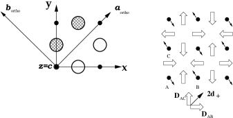
Figure 3: Left: filled (small) circles represent the Cu⁺⁺ ions. The hatched larger circles represent the oxygen O^– ions that are tilted above the CuO₂ layer while the open larger circles are O^– ions that are tilted below the CuO₂ layer, see also Fig. 2. Right: the staggered pattern of the Dzyaloshinskii-Moriya vectors, represented by open arrows along the Cu-Cu bonds, follows from the staggered pattern of the tilting of the oxygen octahedra. Small arrow: in-plane projection of the Cu⁺⁺ spins in the ordered phase.

II Magnetic Group Analysis for La₂CuO₄ and Sr₂CuO₂Cl₂

Before introducing the experimental setup, a preliminary discussion is needed about the point group of La₂CuO₄ and Sr₂CuO₂Cl₂ both in the paramagnetic and antiferromagnetic phases, in order to establish the irreducible co-representations of the Raman tensors. While the paramagnetic case has been already extensively discussed in the literature (see for example Ref. Reehuis, and references therein), a discussion of the magnetic phase is still missing, and we shall briefly review here the basic steps needed to make this analysis.

Let us consider a crystal with a certain symmetry group, ${\bf G}$, and its set of allowed symmetry group operations in the paramagnetic phase, $T>T_{N}$. When the system orders antiferromagnetically, $T<T_{N}$, usually the symmetry is lowered because now not all the sites are equivalent, and the corresponding magnetic group must be determined.Birss In general, two situations can occur:

• Let us call ${\bf H}$ the restricted unitary subgroup of ${\bf G}$ containing the symmetry operations still allowed below $T_{N}$. If ${\bf H}$ is a subgroup of ${\bf G}$ of index 2 (i.e. ${\bf H}$ contains exactly $n/2$ elements of ${\bf G}$) then all the remaining elements of ${\bf G}-{\bf H}$ can nevertheless be promoted to allowed symmetry operations when combined with the time-reversal operation $\theta$, and are thus called anti-unitary elements. One can then identify, for $T<T_{N}$, the magnetic point group corresponding to the classical point group ${\bf G}$ as

  $${\bf M}={\bf H}+\theta({\bf G}-{\bf H}).$$ (4)

• However, it is possible that below $T_{N}$ the unitary operations still allowed form a subgroup ${\bf\cal H}$ of index larger than 2 for ${\bf G}$, but corresponding to a subgroup of index 2 of a different classical group ${\bf\cal G}$ (i.e. ${\bf\cal H}$ contains $r/2<n/2$ elements, where $r$ is the dimension of the group ${\bf\cal G}$). In this case the magnetic group is identified by ${\bf\cal H}$ and the anti-unitary group $\theta({\bf\cal G-H})$, so that

  $${\bf M}={{\bf\cal H}+\theta({\bf\cal G}-{\bf\cal H})}.$$ (5)

II.1 Magnetic point group for La₂CuO₄

The crystal structure of the low temperature orthorhombic phase of La₂CuO₄ is the $Bmab$ structure in Fig. 2, which has as unitary group the $D_{2h}$ point group in the paramagnetic phase $T>T_{N}$. Above the Néel ordering temperature the allowed symmetry operations of the $D_{2h}$ group are

$$D_{2h}=1,{\;}\bar{1},{\;}2_{a},{\;}2_{b},{\;}2_{c},{\;}\bar{2}_{a},{\;}\bar{2}_{b},{\;}\bar{2}_{c},$$ (6)

where the $8$ elements have their usual meaningsBirss : 1= identity; $\bar{1}$= inversion through the symmetry center, which is in this case the central Cu⁺⁺ ion in position 2 of Fig. 2, so that $(a,b,c)\rightarrow(-a,-b,-c)$; $n_{z}$= rotation of $2\pi/n$ around the $z$ axis; $\bar{n}_{z}$= inversion through the symmetry center followed by a $2\pi/n$ rotation around the $z$ axis (note that $\bar{2}_{z}$ corresponds also to a reflexion with a mirror perpendicular to the $z$ axis).

Although it may seem at first that neither $2_{b}$ nor $2_{c}$ are symmetry operations, in both cases the final atomic configurations can be brought back to the original one by a translation of half of the diagonal along the $(011)$ direction (in the $(abc)$ coordinate system). In this sense, the octahedra in position $1$ (front-bottom-left corner) is brought to position $2$ (central ion) and the one from position $2$ is brought to position $3$ (back-top-right corner). Such translation is allowed because there is no way to distinguish the corner and central Cu⁺⁺ ions in the crystal.

Below $T_{N}$, the Cu⁺⁺ ions order antiferromagnetically in the pattern shown in Fig. 2. We can verify that the remaining allowed unitary symmetry operations are

$${\bf H}=1,{\;}\bar{1},{\;}2_{b},{\;}\bar{2}_{b},$$

bearing in mind that a half translation along the $(011)$ diagonal is allowed. We immediately conclude that La₂CuO₄ belongs to the case (a) discussed above, where the subgroup of allowed unitary operations is of index $2$, see Eq. (4). We can now construct the magnetic group of the ordered phase of La₂CuO₄ by combining all the ${\bf G}-{\bf H}$ unitary operations that are not allowed below $T_{N}$ with the time reversal operation $\theta$ (represented in what follows by an underline), thus forming anti-unitary operations. The allowed unitary $+$ anti-unitary operations for La₂CuO₄ below $T_{N}$ are

$${\bf M}={\bf H}+\theta({\bf G}-{\bf H})=1,{\;}\bar{1},{\;}\underline{2}_{a},{\;}2_{b},{\;}\underline{2}_{c},{\;}\bar{\underline{2}}_{a},{\;}\bar{2}_{b},{\;}\bar{\underline{2}}_{c},$$ (7)

such that the magnetic point group for La₂CuO₄ below $T_{N}$ is the

$${\bf M}=\underline{m}m\underline{m}$$

orthorhombic group, which also has $8$ elements. The Raman tensors for such magnetic group are given in terms of the co-representations (see CracknellCracknell )

$$DA_{g}{=}\left(\begin{array}[]{ccc}A&{\rm i}B&0\\ {\rm i}D&E&0\\ 0&0&I\end{array}\right),{\;}\quad DB_{g}{=}\left(\begin{array}[]{ccc}0&0&C\\ 0&0&{\rm i}F\\ G&{\rm i}H&0\end{array}\right),{\;}$$ (14)

where $A,B,C,D,E,F,G,H,I$ are unconstrained real numbers.

II.2 Magnetic point group for Sr₂CuO₂Cl₂

The crystal structure of the high temperature tetragonal (HTT) phase of Sr₂CuO₂Cl₂ is the $I4/mmm$ structure in Fig. 1, which has as unitary group the $D_{4h}$ point group in the paramagnetic phase $T>T_{N}$. Above the Néel ordering temperature the 16 allowed symmetry operations of the $D_{4h}$ group areBirss

$$D_{4h}=1,{\;}\bar{1},{\;}2_{x},{\;}2_{y},{\;}2_{z},{\;}2_{x^{\prime}},{\;}2_{y^{\prime}},{\;}\bar{2}_{x},{\;}\bar{2}_{y},{\;}\bar{2}_{z},{\;}\bar{2}_{x^{\prime}},{\;}\bar{2}_{y^{\prime}},{\;}\pm 4_{z},{\;}\pm\bar{4}_{z},$$

where we used the reference system of Fig. 1. As we can see, the tetragonal character of the unit cell allows for a $4$-fold axis, the $c$-axis, which is perpendicular to the CuO₂ planes (see Fig. 1).

In the antiferromagnetic phase the spin easy-axis is along the $y^{\prime}$ or $(010)$ direction in the $(abc)$ coordinate system, see Fig. 1. Thus, one can easily verify that, below $T_{N}$, $2_{x}$, $2_{y}$, and $\pm 4_{z}$ are no longer symmetry operations, not even when supplemented by the time reversal operation $\theta$. The only allowed unitary operations in the Néel ordered phase of Sr₂CuO₂Cl₂ are

$${\cal H}=1,{\;}\bar{1},{\;}2_{y^{\prime}},{\;}\bar{2}_{y^{\prime}},$$

again bearing in mind that a half translation along the $(011)$ diagonal is allowed. We immediately conclude that Sr₂CuO₂Cl₂ belongs to the case (b) discussed above, as in Eq. (5), where the subgroup $\cal H$ of allowed unitary operations is a subgroup of $D_{4h}$ with index larger than $2$, but it is a subgroup of ${\cal G}=D_{2h}$ ($mmm$) with index $2$. We can now construct the magnetic group of the ordered phase of Sr₂CuO₂Cl₂ by combining all the ${\cal G}-{\cal H}$ unitary operations that are not allowed below $T_{N}$ with the time reversal operation $\theta$, thus forming anti-unitary operations. The allowed unitary $+$ anti-unitary operations for Sr₂CuO₂Cl₂ below $T_{N}$ are

$${\bf M}={{\bf\cal H}+\theta({\bf\cal G}-{\bf\cal H})}=1,{\;}\bar{1},{\;}\underline{2}_{x^{\prime}},{\;}2_{y^{\prime}},{\;}\underline{2}_{z},{\;}\bar{\underline{2}}_{x^{\prime}},{\;}\bar{2}_{y^{\prime}},{\;}\bar{\underline{2}}_{z},$$ (15)

and thus the magnetic group, with only $8$ elements, is again the orthorhombic $\underline{m}m\underline{m}$ group, just like the case of La₂CuO₄.Discussion-NiF2 In fact, when expressed in terms of the $(abc)$ coordinate system of Fig. 1, such that $a\parallel x^{\prime}$, $b\parallel y^{\prime}$, and $c\parallel z$, Eq. (15) can be written:

$${\bf M}=1,{\;}\bar{1},{\;}\underline{2}_{a},{\;}2_{b},{\;}\underline{2}_{c},{\;}\bar{\underline{2}}_{a},{\;}\bar{2}_{b},{\;}\bar{\underline{2}}_{c},$$

which coincides with Eq. (7) above. Thus, to unify the notation we shall use in the following the $(abc)$ coordinate system for both La₂CuO₄ and Sr₂CuO₂Cl₂ while discussing the antiferromagnetic phase. Moreover, since the magnetic group is the same, the Raman tensors are given by Eq. (14) for both systems.

III Inelastic light scattering by magnons in La₂CuO₄ and Sr₂CuO₂Cl₂

One of the possible mechanisms for the inelastic scattering of light by magnetic excitations in crystals is an indirect electric-dipole (ED) coupling via the spin-orbit interaction.Fleury-Loudon Such a mechanism has been in fact used to determine the spectrum of magnetic excitations in many different condensed matter systems like fluorides, XF₂, where X is Mn²⁺, Fe²⁺, or Co²⁺,Fleury-Loudon inorganic spin-Peirls compounds, CuGeO₃,Spin-Pierls and the parent compounds of the high-temperature superconductors.Gozar The Hamiltonian representing the interaction of light with magnons can be written quite generally asCottam-Lockwood

$$H_{ED}=\sum_{{\bf r}}{\bf E}_{S}^{T}\chi({\bf r}){\bf E}_{I},$$

where ${\bf E}_{S}$ and ${\bf E}_{I}$ are the electric fields of the scattered and incident radiation, respectively (${\bf a}^{T}$ is the transposed of the ${\bf a}$ vector) and $\chi({\bf r})$ is the spin dependent susceptibility tensor. We can expand $\chi({\bf r})$ in powers of the spin-operators, ${\bf S}$, as

$$\chi^{\alpha\beta}({\bf r})=\chi^{\alpha\beta}_{0}({\bf r})+\sum_{\mu}K_{\alpha\beta\mu}S^{\mu}({\bf r})+\sum_{\mu\nu}G_{\alpha\beta\mu\nu}S^{\mu}({\bf r})S^{\nu}({\bf r})+\dots,$$

where $\mu,\nu=x,y,z$ label the spin components. The lowest order term $\chi^{\alpha\beta}_{0}({\bf r})$ is just the susceptibility in the absence of any magnetic excitation (it corresponds to elastic scattering), and it will be neglected in what follows. The second and third terms can give rise to one-magnon excitations because they can be written as $S^{\pm}({\bf r})$ and $S^{z}({\bf r})S^{\pm}({\bf r})$, respectively, where here $z$ is the direction of the spin easy-axis. The intensity of the scattering, as well as the selection rules, will be determined by the structure and symmetry properties of the complex tensors $K$ and $G$.

The ED Hamiltonian that describes the ${\bf k}=0$ one-magnon absorption/emission on sublattice A/B can now be written in terms of the $x,y,z$ components of the sublattice magnetization, ${\bf M}_{i}=({\bf S}_{i_{A}}-{\bf S}_{i_{B}})/2$, as

$$H_{ED}=\sum_{i}\left\{{\bf E}_{S}^{T}\chi^{x}{\bf E}_{I}{\;}M^{x}_{i}+{\bf E}_{S}^{T}\chi^{y}{\bf E}_{I}{\;}M^{y}_{i}\right\},$$ (16)

where the matrices $\chi^{x}$ and $\chi^{y}$ are both written in terms of the original $K$ and $G$ tensors. Here we made the usual mean-field assumption $\langle S^{z}_{i_{A}}\rangle=-\langle S^{z}_{i_{B}}\rangle=-S$ and we dropped terms of the type $S_{i_{A}}^{x,y}+S_{i_{B}}^{x,y}$ since these do not contribute for the ${\bf k}=0$ scattering.

III.1 Magnetic excitations and selection rules for La₂CuO₄ and Sr₂CuO₂Cl₂

It is very important to emphasize here that, differently from two-magnon Raman scattering, where the Raman response does not depend on the direction of the spin easy-axis, the one-magnon Raman response does. Indeed, it has been shown by Fleury and LoudonFleury-Loudon that one of the incoming/outgoing components of the electric field must always lie in the direction of the easy axis, and the other one in the perpendicular plane, oriented in the direction of the mode that one wants to probe. In the specific case of La₂CuO₄ and Sr₂CuO₂Cl₂ that we are considering, the easy axis is along $b$. Thus, the only nonvanishing matrix elements for $\chi^{x}\equiv\chi^{a}$, which corresponds to the in-plane or $a$ (DM) mode, are those that mix the spin easy-axis, $b$, with $a$, while for $\chi^{y}\equiv\chi^{c}$, which corresponds to the out-of-plane or $c$ (XY) mode, are those that mix $b$ and $c$. This information allows us to establish: (i) to which magnetic-group co-representation the one-magnon modes belong, and (ii) the precise scattering geometries needed to observe the associated one-magnon Raman modes. For example, it tells us that, for either Sr₂CuO₂Cl₂ or La₂CuO₄, the out-of-plane mode (also referred to as XY modeGozar ; ESR ) belongs to the $DB_{g}$ co-representation of the magnetic point group $\underline{m}m\underline{m}$

$$\chi^{c}\equiv\chi^{XY}=\left(\begin{array}[]{ccc}0&0&0\\ 0&0&{\rm i}F\\ 0&{\rm i}H&0\end{array}\right),{\;}$$ (17)

with $C=G=0$. On the other hand, the in-plane mode (also referred to as DM mode for La₂CuO₄Gozar ; Marcello-Lara ), belongs to the $DA_{g}$ co-representation of the magnetic point group $\underline{m}m\underline{m}$

$$\chi^{a}\equiv\chi^{DM}=\left(\begin{array}[]{ccc}0&{\rm i}B&0\\ {\rm i}D&0&0\\ 0&0&0\end{array}\right),{\;}\quad$$ (18)

with $A=E=I=0$. The precise numerical evaluation of the remaining elements $B,D,F,H$ requires a more detailed microscopic calculation of the electric-dipole induced transitions and spin-orbit coupling in second order perturbation theory, for each system, and this is beyond the scope of this article.

III.2 One-magnon Raman response

According to the electric-dipole Hamiltonian (16), one-magnon Raman scattering probes the long-wavelength spin excitations $M_{i}$ around the staggered spin configuration realized in the antiferromagnetic state. These correspond to the $({\bf k}=0)$ value of the usual spin-wave dispersions, where ${\bf k}$ is measured with respect to the ${\bf Q}=(\pi,\pi)$ vector of the antiferromagentic ordering. In an isotropic Heisenberg antiferromagnet the spin modes are soft at long wavelength, $\omega_{\bf k}\simeq ck$, but for anisotropic spin-spin interactions a gap appears at ${\bf k}=0$, $\omega_{\bf k}=\sqrt{\omega_{a,c}^{2}+c^{2}{\bf k}^{2}}$, where $\omega_{a,c}$ are related to the anisotropy parameters ($\alpha_{a},\alpha_{c}$ in Eq. (1), or to $D_{+},\Gamma$ in Eq. (3)). Starting from the Hamiltonian (16), the Raman response can be obtained using Fermi’s golden rule and, for Stokes scattering, we haveMarcello-Lara

$${\cal I}(\omega)=[n_{B}(\omega)+1]\left\{|\Pi_{a}|^{2}{\cal A}_{a}({\bf 0},\omega)+|\Pi_{c}|^{2}{\cal A}_{c}({\bf 0},\omega)\right\},$$ (19)

where ${\cal I}(\omega)$ is the Raman intensity, $n_{B}(\omega)=(e^{\beta\omega}-1)^{-1}$ is the Bose function and ${\cal A}_{a,c}({\bf 0},\omega)$ is the spectral function of the ${\bf k}=0$ transverse $a/c$ components of the antiferromagnetic (staggered) order parameter. The projectors

$$\Pi_{a,c}={\bf E}_{S}^{T}\chi^{a,c}{\bf E}_{I}$$ (20)

are given in terms of the Raman tensors $\chi^{a,c}$ presented above. The properties of ${\cal A}_{a,c}$ have been extensively discussed in the preceeding paper.LM1 In particular, it has been shown that the spectral function ${\cal A}_{a,c}({\bf 0},\omega)$ is peaked at the energy $\omega_{a,c}(H)$ of the magnon gaps in magnetic field, with an intensity $I_{a,c}$ which also depends on $H$. For La₂CuO₄, $\omega_{a}$ corresponds to the Dzyaloshinskii-Moriya gap, while for Sr₂CuO₂Cl₂ it corresponds to the in-plane gap, as discussed in the introduction. For both compounds, $\omega_{c}$ corresponds to the XY anisotropy gap.

IV Experimental Setup

Single crystals of La₂CuO₄ and Sr₂CuO₂Cl₂Lance were measured in a backscattering geometry with the incoming photons propagating along the $c$ crystallographic axis. The polarization configurations are denoted by $({\bf E}_{I},{\bf E}_{S})$ with ${\bf E}_{I/S}$ representing the direction of the incoming/scattered electric field. The crystals were mounted in a continuous flow optical cryostat and the Raman spectra were taken using about 5mW power and the wavelength $\lambda=647.1$ nm from a Kr⁺ laser. The measurements in magnetic fields were taken with the cryostat inserted in a room temperature horizontal bore of a superconducting magnet. The orthorhombic axes of the La₂CuO₄ sample were identified by X-ray diffraction. The data from Sr₂CuO₂Cl₂ crystal were taken from a freshly cleaved $(ab)$ surface but in this case the in-plane axes directions were not determined.

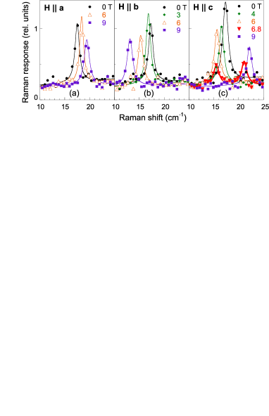
Figure 4: (Color online) One-magnon Raman response for La₂CuO₄ at $T=10$ K in the $(RL)$ circular polarization configuration, where only the Dzyaloshinskii-Moriya gap is Raman active. In $(a)$ the gap only hardens, in $(b)$ the gap only softens, while in $(c)$ it first softens and then hardens above the weak-ferromagnetic transition at $H\simeq 6.6$ T (see discussion in the text).

We first present the one-magnon Raman response in La₂CuO₄ for the $(RL)$ polarization configuration. In this geometry, the electric-field of the incident light is circularly polarized rotating clockwise, ${\bf E}_{I}^{R}=(\hat{\bf x}_{a}-{\rm i}\hat{\bf x}_{b})/\sqrt{2}$, while the electric-field of the scattered light is circularly polarized and rotating anti-clockwise, ${\bf E}_{S}^{L}=(\hat{\bf x}_{a}+{\rm i}\hat{\bf x}_{b})/\sqrt{2}$. Here $\hat{\bf x}_{a}$ and $\hat{\bf x}_{b}$ are unit vectors along the $a$ and $b$ directions respectively. According to our earlier discussion on the classification of the magnetic excitations in La₂CuO₄, the $(RL)$ in-plane polarization configuration is the adequate Raman geometry in order to observe the Dzyaloshinskii-Moriya gap, because it probes directly the nonvanishing element $B,D$ of the $\chi^{DM}$ matrix (18). The results are presented in Fig. 4. In $(a)$ the magnetic field is applied along the $a$ axis (transverse field). We observed a monotonic hardening of the gap with increasing magnetic field. In $(b)$ the magnetic field is applied along the $b$ axis (longitudinal field). We observed a monotonic softening of the gap with increasing magnetic field. Finally, in $(c)$ the magnetic field is applied perpendicular to the CuO₂ layers (transverse field). We observed first a softening of the gap with increasing field, a jump at a field of approximately $6.6$ T, and finally a hardening with increasing field.

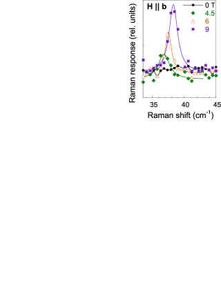
Figure 5: (Color online) One-magnon Raman response for La₂CuO₄ at $T=10$ K in the $(RR)$ circular polarization configuration for a magnetic field applied along the orthorhombic $b$ easy-axis, where the field-induced mode becomes Raman active (see discussion in the text). We observed a monotonic hardening of the field-induced mode with increasing applied field.

Next we present the one-magnon Raman response in La₂CuO₄ for the $(RR)$ polarization configuration. In this geometry, the electric-field of both the incident and scattered light is circularly polarized rotating anti-clockwise, ${\bf E}_{I}^{R}={\bf E}_{S}^{R}=(\hat{\bf x}_{a}+{\rm i}\hat{\bf x}_{b})/\sqrt{2}$. According to the theory described in Ref. Marcello-Lara, , the $(RR)$ in-plane polarization configuration is the adequate Raman geometry in order to observe the field-induced mode for a magnetic field applied along the orthorhombic $b$ easy-axis, because it probes directly the nonvanishing elements of the rotated $\chi^{XY}_{\theta}$ matrix

$$\chi^{XY}_{\theta}=\left(\begin{array}[]{ccc}0&0&0\\ 0&{\rm i}(F+H)\sin\theta\cos\theta&-{\rm i}H\sin^{2}\theta+{\rm i}F\cos^{2}\theta\\ 0&-{\rm i}F\sin^{2}\theta+{\rm i}H\cos^{2}\theta&-{\rm i}(F+H)\sin\theta\cos\theta\end{array}\right),{\;}$$ (21)

where $\theta$ is the angle of rotation of the spin-quantization basis within the $(bc)$ plane.Marcello-Lara The $(RR)$ polarization configuration then probes the element ${\rm i}(F+H)\sin\theta\cos\theta$. The results are presented in Fig. 5 and we observed a monotonic hardening of the gap with increasing magnetic field. Only the data points for higher fields are shown in Fig. 5 because the intensity of the peak rapidly drops for fields lower than $4$ T.

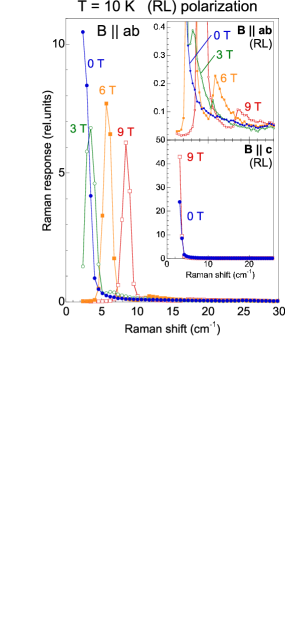
Figure 6: (Color online) One-magnon Raman response for Sr₂CuO₂Cl₂ at $T=10$ K in the $(RL)$ polarization configuration, where only the in-plane gap is Raman active. Main figure: hardening of the in-plane gap with increasing in-plane magnetic field. Insets: (top) zoomed immage of the main plot, showing the much weaker intensity of the two-magnons scattering, starting at approximately twice the magnon gap; (bottom) featureless response for perpendicular magnetic field (the out-of-plane (XY) mode is not Raman active in the backscattering geometry used here).

Finally we present the one-magnon Raman response in Sr₂CuO₂Cl₂ also for the $(RL)$ polarization configuration. The results are presented in Fig. 6. First, we observe that at zero applied field the Raman spectrum is continuously increasing up to the lowest accessible frequency of 2 cm^-1. As a consequence, we can only establish an upper bound of 2 cm^-1 for the in-plane magnon gap. This very small value is consistent with the general expectation that the in-plane gap for Sr₂CuO₂Cl₂ has a purely quantum origin. When the magnetic field is in the plane (main panel) one observes a hardening of the one-magnon peak, which allows us to clearly identify the magnon gap as the field increases, while no changes are observed for a magnetic field parallel to $c$ (bottom inset). Observe also (top inset) that the signal corresponding to the two-magnon continuum (which starts at the edge of approximately twice the magnon gap) has much lower intensity with respect to the one-magnon peak.

V Magnetic spectrum in La₂CuO₄

V.1 ${\bf H}$ parallel to $a$

For a field applied parallel to the $a$ orthorhombic axis, we obtain the conventional field dependence of the magnon gaps in a transverse field:LM1 the hardening of the mode in the field direction, while the second mode remains unchanged

$$\omega_{a}(H)=\sqrt{m^{2}_{a}+(g_{s}^{a}\mu_{B}H)^{2}},\quad\omega_{c}(H)=m_{c}.$$ (22)

Here we indicate with $m_{a},m_{c}$ the gaps of the magnon modes at zero field, $\omega_{a}(0)=m_{a}$ and $\omega_{c}(0)=m_{c}$. Moreover, with respect to the preceding article,LM1 we restored the physical units for the magnetic field, introducing the Bohr magneton $\mu_{B}=0.4668$ cm^-1T^-1 and the gyromagnetic ratio $g_{s}^{a}$ for the field along $a$. We then obtain for the $\omega_{a}$ mode the relation

$$\omega_{a}^{2}=m_{a}^{2}+\gamma_{a}H^{2},\quad\gamma_{a}=(g_{s}^{a}\mu_{B})^{2}.$$ (23)

As one can see in Fig. 7, the data for $\omega_{a}({\bf H}\parallel a)$ follow perfectly the previous equation, with a coefficient $\gamma_{a}^{F}=0.93$ (cm T)^-2 estimated by fitting the data with Eq. (23). This value allows us to estimate the gyromagnetic ratio as:

$$g_{s}^{a}=\sqrt{\gamma_{a}^{F}}/\mu_{B}=2.0,$$ (24)

in good agreement with the estimate given usually in the literature.

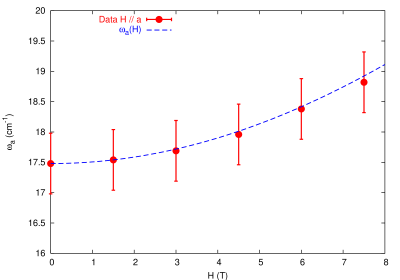
Figure 7: (Color online) Comparison between the experimental data and theoretical predictions for the field dependence of the DM gap for ${\bf H}\parallel a$. The closed circles are the experimental data. The line is the best fit obtained using Eq. (23), with $\gamma_{a}^{F}=0.93$ (cm T)^-2.

V.2 ${\bf H}$ parallel to $c$

When the field is applied along the $c$ direction one observes a spin-flop of the ferromagnetic spin components along $c$, which are ordered antiferromagnetically in neighboring planes at low fieldLM1 ; Thio90 ; Papanicolaou . This weak ferromagnetic (WF) transition has been indeed measured in Ref. [Magnetoresistence, ] for the $x=0.01$ doped compound, occuring at a temperature-dependent critical field of about 4 T at $T=50$ K. Since the magnitude of the ferromagnetic spin components along $c$ decreases with the temperature proportionally to the AF order parameter $\sigma_{0}$, also the critical field $H_{c}$ for the WF transition decreases with temperature. By properly taking into account the effect of quantum and thermal fluctuations on the order parameter one can determine the $H_{c}(T)$ curve reported in Fig. 8,LM1 where we also sketch the spin configuration above and below the transition. However, as it has been discussed in Ref. LM1, , a first estimate for the critical field at low temperature and for the field dependence of the magnon gaps can be obtained by neglecting the renormalization of $\sigma_{0}$. Using the notation of Ref. LM1, , we will decompose the spin at site $i$ in its staggered ${\bf n}$ and uniform ${\bf L}$ component, so that ${\bf S}_{i}/S=e^{i{\bf Q}\cdot{\bf r}_{i}}{\bf n}_{i}+a{\bf L}$. In the AF ordered state $\langle{\bf n}\rangle=\sigma_{0}$, where in general $\sigma_{0}$ is corrected both by quantum and thermal corrections. At low temperatures, and neglecting quantum fluctuations $(\sigma_{0}=1)$, one obtains that the critical field is

$$H_{c}=\frac{2\eta}{g_{s}^{c}\mu_{B}D_{+}},$$ (25)

where $\eta=2JJ_{\perp}$ is the energy scale associated to the interlayer coupling $J_{\perp}$, and $D_{+}$ is the modulus of the DM vector, which controls also the ${\bf H}=0$ value of the DM gap, $D_{+}\equiv m_{a}$LM1 .

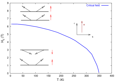
Figure 8: (Color online) Phase diagram of the weak-ferromagnetic transition and spin configuration for $H\parallel c$. The arrows with open tip represent the spins in each layer, the small ones on the right of the layers the uniform spin components. At low temperature and zero or low field the uniform components of the spins in each layers are ordered antiferromagnetically in the $c$ direction. Above the critical field (25) the uniform components order ferromagnetically in the $c$ direction. As the temperature increases the uniform components decrease follwing the decrease of the AF spin component along $b$, and as a consequence also the critical field for the WF transition decreases. The phase diagram has been calculated in Ref. [LM1, ] (see Fig. 10) by using parameter values appropriate for La₂CuO₄.

According to the analysis of Ref. LM1, , the magnon gaps evolve, below $H_{c}$, as

$$\omega^{2}_{a} = m_{a}^{2}+2\eta-\sqrt{4\eta^{2}+\left(g_{s}^{c}\mu_{B}HD_{+}\right)^{2}},$$

$$\omega^{2}_{c} = m_{c}^{2}+(g_{s}^{c}\mu_{B}H)^{2}+2\eta-\sqrt{4\eta^{2}+\left(g_{s}^{c}\mu_{B}HD_{+}\right)^{2}},\quad H<H_{c},$$ (26)

while above the WF transition they are given by

$$\omega^{2}_{a} = m_{a}^{2}+|g_{s}^{c}\mu_{B}HD_{+}|,$$

$$\omega^{2}_{c} = m_{c}^{2}+(g_{s}^{c}\mu_{B}H)^{2}+|g_{s}^{c}\mu_{B}HD_{+}|,\quad H>H_{c}.$$ (27)

Using this set of equations we recognize that the parameter $\eta$ can be determined from the jump of the gap at $H_{c}$, since

$$\omega^{2}_{a}(H_{c}^{-})=m_{a}^{2}-2\eta(\sqrt{2}-1),\quad\omega^{2}_{a}(H_{c}^{+})=m_{a}^{2}+2\eta.$$

We can then estimate

$$2\eta=\frac{\omega^{2}_{a}(H_{c}^{+})-\omega^{2}_{a}(H_{c}^{-})}{\sqrt{2}}=143.25\,{\mathrm{c}m}^{-2},$$ (28)

from which it follows also that

$$\eta=2JJ_{\perp}\Rightarrow J_{\perp}/J\sim 3.2\times 10^{-5},$$ (29)

where we used $J=130$ meV. We can then recognize that the field evolution of the $\omega_{a}$ gap above and below the WF transition is controlled by a single parameter $\gamma_{c}$

$$\omega^{2}_{a} = m_{a}^{2}+2\eta-\sqrt{4\eta^{2}+(\gamma_{c}H)^{2}},\quad H<H_{c}$$

$$\omega^{2}_{a} = m_{a}^{2}+\gamma_{c}H,\quad H>H_{c},$$ (30)

where $\gamma_{c}$ is uniquely determined by $2\eta$, $H_{c}$ and the gyromagnetic ratio of the $c$ direction $g_{s}^{c}$

$$\gamma_{c}=g_{s}^{c}\mu_{B}D_{+}=\frac{2\eta}{H_{c}}.$$ (31)

As a consequence, we can extract $g_{s}^{c}$ both by fitting the experimental data with Eqs. (30) and obtaining a value $\gamma_{c}^{F}$, and by using directly the last two equalities of Eq. (31). In the former case we obtain $\gamma_{c}^{F}=$ 21.83 cm^-2T^-1, which corresponds to $g_{s}^{c}=2.7$. In the latter case instead we can use the value of $2\eta$ obtained from the jump of the gap at $H_{c}$, the value $D_{+}=m_{a}=17.48$ cm^-1, and the measured value $H_{c}\simeq 6.6$ T, finding

$$g_{s}^{c}=\frac{2\eta}{\mu_{B}H_{c}D_{+}}=2.65.$$ (32)

Thus, both estimates give a value which is quite close to the one commonly quoted in the literature, $g_{s}^{c}=2.45$.

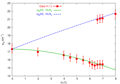
Figure 9: (Color online) Comparison between the experimental data and the theoretical predictions for the field dependence of the DM gap for ${\bf H}\parallel c$. The closed circles are the experimental data. Observe that near the WF transition two values of the gap have been measured (see also panel (c) of Fig. 4). Indeed, since the transition is first order in a finite sample the transition is observed as a coexistence of the two phases (above and below the transition) for a range of field values around the thermodynamic critical field. The lines are the fit using Eqs. (30), with $\gamma_{c}^{F}=21.83$ cm^-2T^-1.

Observe that this value of $g_{s}^{c}$ is only an upper bound because we did not include in the set of Eqs. (30) and in the definition of the critical field (25) the quantum and thermal correction of the order parameter $\sigma_{0}$, which reduce its value with respect to $\sigma_{0}=1$ used so far. As it has been explained in Ref. LM1, , when this effect is taken into account one must replace $D_{+}$ by $D_{+}/\sigma_{0}$ in Eqs. (26)-(27)

$$\omega^{2}_{a} = m_{a}^{2}+2\eta-\sqrt{4\eta^{2}+\left(\frac{g_{s}^{c}\mu_{B}HD_{+}}{\sigma_{0}}\right)^{2}},$$

$$\omega^{2}_{c} = m_{c}^{2}+(g_{s}^{c}\mu_{B}H)^{2}+2\eta-\sqrt{4\eta^{2}+\left(\frac{g_{s}^{c}\mu_{B}HD_{+}}{\sigma_{0}}\right)^{2}},\quad H<H_{c},$$ (33)

and

$$\omega^{2}_{a} = m_{a}^{2}+\left(\frac{g_{s}^{c}\mu_{B}HD_{+}}{|\sigma_{0}|}\right),$$

$$\omega^{2}_{c} = m_{c}^{2}+(g_{s}^{c}\mu_{B}H)^{2}+\left(\frac{g_{s}^{c}\mu_{B}HD_{+}}{|\sigma_{0}|}\right),\quad H>H_{c}.$$ (34)

At the same time the critical field is a function of $\sigma_{0}$ according to

$$H_{c}=\frac{4\eta}{g_{s}^{c}\mu_{B}D_{+}}\frac{\sigma_{0}}{1+\sigma_{0}^{2}}.$$ (35)

The order parameter $\sigma_{0}$ is determined at each temperature by computing the effect of transverse spin-wave fluctuations, which depends on the magnon gap according to a general equation like

$$\sigma_{0}^{2}(H,T)=1-I_{\perp}(\omega_{a}(H),\omega_{c}(H),T),$$ (36)

where the precise expression for $I_{\perp}$ is given in Ref. LM1, . Note that since the DM interaction introduces an explicit dependence of the magnon gaps on the order parameter, see Eqs. (33)-(34), Eq. (36) is a self-consistency equation for $\sigma_{0}$. As far as the previous estimates of $\eta$ and $g_{s}^{c}$ are concerned, one can see that the solution of the full set of Eqs. (33)-(34) (35) and (36) can slightly modify the values previously obtained in two respects. First, the jump of the gap at the critical field will depend not only on $\eta$ but also on $\sigma_{0}$. Second, the analogous of Eq. (32) will be

$$g_{s}^{c}=\frac{4\eta}{\mu_{B}H_{c}D_{+}}\frac{\sigma_{0}}{1+\sigma_{0}^{2}}.$$ (37)

Observe that both these corrections will contribute to a reduction of $g_{s}^{c}$ with respect to the previous estimate. However, since the experimental determination of $\sigma_{0}$ in this sample is not available and the theoretical value depends on the approximations used to derive Eq. (36), we retain here the estimates given above using $\sigma_{0}=1$ and we refer the reader to Ref. LM1, for a more detailed discussion of this issue.

We should point out that a somewhat larger estimate for the critical field $H_{c}$ has been extracted recently from the neutron scattering measurements of Ref. Reehuis, , in a La₂CuO₄ sample with almost the same Néel temperature as the one considered here. According to the previous Eq. (35), several factors can affect the critical field. Thus, the larger critical field measured in the sample of Ref. Reehuis, can be explained with a larger value of the staggered order parameter and of the interlayer coupling $\eta$, or also with a smaller value of the DM vector $D_{+}$. However, one should remember that the weak-ferromagnetic transition for $H\parallel c$ is a first-order transition accompanied by a hysteresis that can be large at low temperature (see for example Ref. Magnetoresistence, ), and hence the experimentally determined critical field could be affected by the hysteresis. As a consequence, further investigation of the parameter values for this sample can shed more light on this apparent discrepancy between the Raman and the neutron scattering measurements.

V.3 ${\bf H}$ parallel to $b$

Finally, let us discuss the case of ${\bf H}\parallel b$, where also the data for the field-induced mode $\omega_{c}$ are available for $H\geq 4$ T. Here again the field dependence of the magnon gaps follows a different behavior for small and large field. As it has been explained in Ref. LM1, , due to the DM interaction a field along $b$ generates an effective staggered field in the $c$ direction, giving rise to a rotation of the staggered order parameter in the $bc$ plane.Reehuis As a consequence, at low field the classical configuration of the staggered AF order parameter ${\bf n}_{m}$ in the $m$-th plane is given by

$${\bf n}_{m}=(0,\sigma_{b},(-1)^{m}\sigma_{c}).$$ (38)

where $\sigma_{b}$ and $\sigma_{c}$ indicate, respectively, the components of the order parameter along $b$ and $c$ direction. Observe that an oscillating staggered $\sigma_{c}$ component implies that in the spin decomposition ${\bf S}_{i}/S=e^{i{\bf Q}\cdot{\bf r}_{i}}{\bf n}_{i}+{\bf L}_{i}$ given above actually the $S^{c}$ components coming from $n^{c}$ are ordered ferromagnetically in neighboring planes, to allow for the (average) uniform spin components ${\bf L}$ induced by the DM vector to align along the applied field.LM1

As the field strenght increases, the spins perform a two-step spin-flop transition:LM1 ; Thio90 ; Papanicolaou at $H=H_{c}^{(1)}$ the in-plane AF components allign along the $a$ direction, while at $H=H_{c}^{(2)}>H_{c}^{(1)}$ the $a$ component vanishes and only the staggered spin components in the $c$ direction are left. In Fig. 10 we shown the $(H-T)$ phase diagram which has been evaluated in Ref. [LM1, ] by means of a saddle-point approximation for the transverse spin fluctuations. The temperature $T_{N}$ is the one where the in-plane spin component (along $b$ or $a$) vanishes, leaving a non-zero $\sigma_{c}$ component. Observe that the jump of $T_{N}(H)$ at $H_{c}^{(1)}$ is an artifact of the approximation: indeed, the critical field for this transition is controlled by the energy scale where the $\omega_{a}$ gap vanishes (see Eq. (40) below), i.e.

$$g_{s}^{b}\mu_{B}H_{c}^{(1)}=m_{a}=D_{+},$$ (39)

which corresponds, in our case, to $H_{c}^{(1)}=18$ T. Since within the saddle-point approximation $m_{a}$ is temperature independent, at this level one cannot recover the temperature variation of $H_{c}^{(1)}$ which would eliminate the anomalous jump of $T_{N}(H)$ reported in Fig. 10. Since the maximum field used in the present experiments is $H=11$ T, this spin flop transition is out of the range accessible in our measurements. It is perhaps worth pointing out that in a recent work the evolution of the magnetic signal for $H\parallel b$ has been measured by means of neutron scattering up to fields of 14 T.Reehuis By assuming a power-law decay of the intensity of the $(100)$ neutron peak - corresponding to magnetic order along the $b$ direction - the authors could estimate for the above critical field a slightly higher value of $22$ T. Considering that a theoretical prediction of the neutron-peak intensity as a function of magnetic field is still lacking, this estimate seems in good agreement with the value (39) given above.

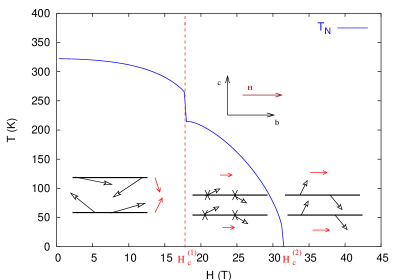
Figure 10: (Color online) Phase diagram and evolution of the spin configuration for $H\parallel b$. For the spin components we use the same notation as in Fig. 8 above. At $H<H_{c}^{(1)}$ both the spins and the uniform components rotate in the $bc$ plane, so that the net uniform magnetization in along the $b$ axis. In this region $T_{N}(H)$ is the temperature at which the in-plane AF component along $b$ vanishes. At $H_{c}^{(1)}<H<H_{c}^{(2)}$ the AF spin components allign along $a$ which is perpendicular to the plane of the figure, so that these spin components, which vanish at the temperature $T_{N}(H)$, are represented by the small crosses. At the same time, the uniform components align ferromagnetically in neighboring planes. At $H>H_{c}^{(2)}$ only the $c$ components survive.

As far as the magnon-gap evolution with magnetic field is concerned, at field below $H_{c}^{(1)}$ it is the usual one for longitudinal fieldsLM1

$${\omega_{a}^{2}}=\frac{m^{2}_{a}+m_{c}^{2}}{2}+(g_{s}^{b}\mu_{B}H)^{2}-\sqrt{\left(\frac{m^{2}_{a}-m_{c}^{2}}{2}\right)^{2}+4(g_{s}^{b}\mu_{B}H)^{2}\left(\frac{m^{2}_{c}+m_{a}^{2}}{2}\right)},$$

$${\omega_{c}^{2}}=\frac{m^{2}_{a}+m_{c}^{2}}{2}+(g_{s}^{b}\mu_{B}H)^{2}+\sqrt{\left(\frac{m^{2}_{a}-m_{c}^{2}}{2}\right)^{2}+4(g_{s}^{b}\mu_{B}H)^{2}\left(\frac{m^{2}_{c}+m_{a}^{2}}{2}\right)}.$$ (40)

At small field these expressions can be approximated as

$$\omega^{2}_{a}=m_{a}^{2}-\gamma_{a}H^{2},\quad\gamma_{a}=(g_{s}^{b}\mu_{B})^{2}\Delta m^{a},\quad\Delta m^{a}=\left[2\frac{m^{2}_{c}+m^{2}_{a}}{m^{2}_{c}-m^{2}_{a}}-1\right]$$ (41)

$$\omega^{2}_{c}=m_{c}^{2}+\gamma_{c}H^{2},\quad\gamma_{c}=(g_{s}^{b}\mu_{B})^{2}\Delta m^{c},\quad\Delta m^{c}=\left[2\frac{m^{2}_{c}+m^{2}_{a}}{m^{2}_{c}-m^{2}_{a}}+1\right]$$

Using Eq. (40) and the zero-field value of the $a$ mode we obtain again an excellent agreement with the experimental points, as one can see in Fig. 11. For the sake of completeness we also report in Fig. 11 the approximate expression (41), which is indeed valid until the field $H_{l}\simeq 4$ T. From the fit of the $\omega_{a}$ data using Eqs. (40) we obtain both $m_{c}=\omega_{c}(H=0)$ and the gyromagnetic ratio. The results are

$$m_{c}=36\,\mathrm{cm}^{-1},\quad g_{s}^{b}=2.08,$$ (42)

which are again in excellent agreement with the values reported in the literature.

In the inset of Fig. 11 we show also the field dependence of the field-induced $\omega_{c}$ (XY) mode according to Eq. (40), using the values (42) extracted from the fitting of the $\omega_{a}$ mode. As one can see, only the data point at $9$ T is out of the range of the thoeretical curve. The appearence of the field-induced $\omega_{c}$ mode for the in-plane Raman scattering in the $(RR)$ polarization configuration is now well understood as being a consequence of a continuous rotation of the magnetization axis when ${\bf H}\parallel b$.Marcello-Lara

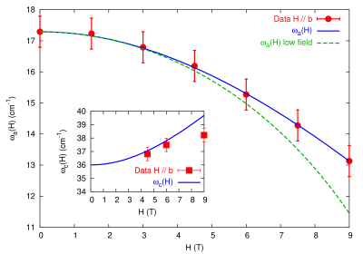
Figure 11: (Color online) Comparison between the experimental data and the theoretical predictions for the field dependence of the $a$ mode for ${\bf H}\parallel b$. The blue solid line is the fit done using the first of Eqs. (40) with $g_{s}$ and $m_{c}$ as fitting parameters, giving $g_{s}^{b}=2.08$ and $m_{c}=36$ cm^-1. The green dashed line is the approximated expression (41) evaluated with the same parameters values, and it is only valid at low field. Inset: field dependence of the $c$ mode observed at fields larger than 4 T. The solid line is the curve corresponding to the second of Eqs. (40).

V.4 Peak intensity as a function of magnetic field

A complete microscopic theory of the Raman scattering which allows one to compute the exact shape and the absolute intensity of the Raman peaks is out of the scope of the present paper. Nonetheless, when data taken at different magnetic fields are compared, one could expect that the main dependence of the relative peak intensity measured by Raman can be at least qualitatively described by the theory developed in Ref. LM1, . Indeed, the spectral function ${\cal A}_{a,c}$ contains itself an intrinsic dependence of the peak intensity on the magnetic field, which enters in the Raman response trough the relation (19). Thus, we can evaluate Eq. (19) using the theoretical prediction for ${\cal A}_{a,c}$ and compare it with the experimental data. As we shall see, even though our analysis does not include the spin damping processes, the overall agreement between the theoretical predictions and the experimental data is fairly good.

As it has been discussed in Ref. LM1, , the spectral function of each mode is defined from the Green’s function for the corresponding fluctuations. In the absence of magnetic field the Green’s function for the transverse mode is a diagonal matrix

$$\hat{G}^{-1}=\frac{1}{gc}\left(\begin{array}[]{cc}\omega_{n}^{2}+\varepsilon_{a}^{2}({\bf k})&0\\ 0&\omega_{n}^{2}+\varepsilon_{c}^{2}({\bf k})\end{array}\right),$$ (43)

where the magnon gap is by definition $\omega_{a,c}=\varepsilon_{a,c}({\bf k}=0)$. In this case the Green’s function matrix is also diagonal and we simply obtain

$${\cal A}_{a}(\omega>0)=-\frac{1}{\pi}ImG_{a}(i\omega_{n}\rightarrow\omega+i0^{+})=\frac{1}{2\omega_{a}}\delta(\omega-\omega_{a}),$$ (44)

and analogously for ${\cal A}_{c}$. Thus, from Eq. (44) we can deduce that the peak intensity $I_{a}$ evolves as $1/\omega_{a}$, i.e. it is larger for smaller gap values.

When a magnetic field is applied, two different cases must be considered: (i) if the matrix $\hat{G}$ is still diagonal the structure (44) of the spectral function is preserved, and both the peak position and its intensity evolve as $\omega_{a,c}(H)$, and $I_{a}=1/\omega_{a,c}(H)$, respectively; (ii) if off-diagonal terms proportional to the magnetic field appear in Eq. (43) the Green’s function of the transverse fluctuations has a non-diagonal structure which leads to the appearance of several magnon gaps in the response of each single mode. For example, in the case of longitudinal field one has for the spectral function of the $a$ mode a structure likeLM1

$${\cal A}_{a}(\omega>0)=\left[\frac{Z_{a}}{2\omega_{a}}\delta(\omega-\omega_{a})+\frac{Z_{c}}{2\omega_{c}}\delta(\omega-\omega_{c})\right].$$ (45)

However, one finds in general that $Z_{a}/\omega_{a}\gg Z_{c}/\omega_{c}$, so that essentially a single peak at the $\omega_{a}$ energy is observed in the measurements, but the spectral weight of this peak is $I_{a}=Z_{a}/\omega_{a}$ and not just $1/\omega_{a}$ as in Eq. (44). Indeed, the factor $Z_{a}$ in Eq. (45) leads in general to an additional field dependence of the intensity on the magnetic field.

For an ordinary easy-axis AF Eq. (44) is valid when a transverse field is applied, so that an hardening of the gap in the field direction should be also accompanied by a softening of the peak intensity. For a longitudinal field one finds instead the spectral function (45) given above. According to the calculations of Ref. LM1, , $Z_{a}$ is given by

$$Z_{a}=\frac{-\omega^{2}_{a}+m^{2}_{c}-H^{2}}{\omega_{c}^{2}-\omega_{a}^{2}},$$ (46)

and it is a decreasing function of the magnetic field. As a consequence, the overall factor $Z_{a}/\omega_{a}$ in Eq. (45) is increasing much more slowly than the $\sim 1/\omega_{a}$ behavior that one could expect for a transverse gap, as it is shown in Fig. 12. Here, according to Eq. (19), we included also the bose factor $[n_{B}(\omega)+1]$, whose contribution to the overall dependence of the peak intensity is however very small.

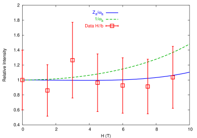
Figure 12: (Color online) Field dependence of the normalized intensity $I_{a}(H)/I_{a}$ of the $a$ peak for a longitudinal field. We estimated the relative error on the measured peak intensity around 20 $\%$. Solid line: field dependence of the peak intensity according to Eqs. (45) and (46). Observe that by neglecting the contribution of the $Z_{a}$ factor from Eq. (46) one would obtain $I_{a}=1/\omega_{a}$, corresponding to the dashed line, which shows an increasing of the relative intensity not observed in the experiments.

In the case of ${\bf H}\parallel c$ in an ordinary easy-axis AF one would expect the peak for the $a$ to be unchanged, as indeed observed in Sr₂CuO₂Cl₂. However, for La₂CuO₄ the presence of the DM interaction does modify both the peak position and its intensity as a function of magnetic field. Below the critical field for the spin-flop transition the spectral function of the $a$ mode isLM1

$${\cal A}_{a}(\omega>0)\approx\frac{Z_{a}}{\omega_{a}}\delta(\omega-\omega_{a}),$$ (47)

where

$$Z_{a}=\frac{2\eta+\sqrt{4\eta^{2}+(HD_{+}/\sigma_{0})^{2}}}{2\sqrt{4\eta^{2}+(HD_{+}/\sigma_{0})^{2}}}.$$ (48)

Once again, while the $1/\omega_{a}(H)$ increases with magnetic field the $Z_{a}$ factor decreases, giving rise to an almost constant spectral weight below the spin-flop transition, see Fig. 13. Here we used the $\eta$ value extracted from the fit with $\sigma_{0}=1$. Above the spin-flop transition the matrix of the transverse fluctuations is again diagonal and the standard $I_{a}=1/\omega_{a}$ spectral weight is expected, with the $\omega_{a}(H)$ dependence given by Eq. (34).

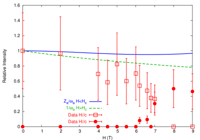
Figure 13: (Color online) Field dependence of the intensity of the $a$ peak for a transverse field in the $c$ direction. Observe that the spin-flop WF transition is first order, so that by increasing the magnetic field one first access a crossover regime where the Raman intensity is split between the two peaks corresponding to the equilibrium gap values at $H<H_{c}$ and $H>H_{c}$. Thus, only the data at $H>7$ T should be compared with the dashed curve, corresponding to the state above the spin flop.

VI Magnetic Spectrum in Sr₂CuO₂Cl₂

The case of Sr₂CuO₂Cl₂ is rather simple. This system is very well described by the Hamiltonian (1) with a large XY anisotropy $\alpha_{c}\sim 10^{-4}J$. Since the system is tetragonal, one does not have in principle any intrinsic in-plane anisotropy, i.e. one would expect $\alpha_{a}=0$ in this case. Nonetheless, it has been suggested in Ref. Yildirim, that a very small in-plane gap can still exist as due to purely quantum effects. Recent ESR measurements seem to confirm this prediction and give an estimate of the in-plane gap as $m_{a}=0.048\sim 0.05$ meV.ESR As we can see from Fig. 6 there might be a peak at low energies (below 2 cm^-1 for $H=0$ T), which can well correspond to the same in-plane gap as observed by ESR. As far as the field dependence of the gaps is concerned, the results obtained in the Sec. III-IV of the preceding article for a conventional easy-axis AF still apply.LM1 Moreover, since no orthormonbic distortion exists in Sr₂CuO₂Cl₂, no DM interaction is present, and no effects due to staggered fields will show up in the field dependence of the magnon gaps.

In Fig. 14 we compare the extracted dispersion of the in-plane gap in Sr₂CuO₂Cl₂ for an applied magnetic field parallel to the CuO₂ layers, with the predictions for a transverse magnetic field from the theory presented in the preceding articleLM1

$${\omega_{a}}(H)=\sqrt{m_{a}^{2}+(g_{s}\mu_{B}H)^{2}}.$$ (49)

As we can see, by using the value of the gap given by the ESR measurements, $m_{a}=0.048\sim 0.05$ meV,ESR and $g_{s}=2.05$ the agreement is already quite good. On the other hand, we can use the Raman data alone to give an independent estimate of both $m_{a}$ and $g_{s}$, in the same spirit of the previous Sections. This is shown in Fig. 14, and the best fit is for $g_{s}=1.98$ and $m_{a}=1.96$ cm^-1 ($m_{a}=0.24$ meV). Observe that this estimate of $m_{a}$ is larger than the one measured by ESR, but it is still consistent with the fact that at $H=0$ no gap was observed in the Raman spectra at frequency larger than 2 cm^-1, which is the lower bound of the accessible frequency range as shown in Fig. 6.

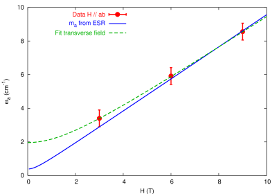
Figure 14: (Color online) Field dependence of the in-plane spin-wave gap measured by Raman in Sr₂CuO₂Cl₂. Solid line: field dependence of the $a$ gap obtained using the value $m_{a}=0.4$ cm^-1 and $g_{s}=2.05$ measured by ESR and the theoretical prediction for a transverse field. Dashed line: best fit on the data point using Eq. (49) with $m_{a}$ and $g_{s}$ as fitting parameters.

Finally, we should emphasize that no field-induced modes were observed in Sr₂CuO₂Cl₂ neither for perpendicular nor in-plane magnetic fields. This results from the absence of the Dzyaloshinskii-Moriya interaction in Sr₂CuO₂Cl₂. In fact, it is exactly the DM interaction in La₂CuO₄ that causes the rotation of the spin-quantization basis and modifies the Raman selection rules allowing for the appearance of a field-induced mode when the field is along the easy axis.Marcello-Lara Moreover, the DM interaction is responsible for the in-plane gap evolution for a field along $c$, which is instead unexpected in a conventional easy-axis antiferromagnet.

VII Conclusions

We have measured, discussed, and compared the one-magnon Raman spectrum of Sr₂CuO₂Cl₂ and La₂CuO₄. We have seen that, for the case of Sr₂CuO₂Cl₂, which is a conventional easy-axis antiferromagnet, there is an in-plane magnon mode at very low energies in the $DA_{g}$ channel that is accessible in the $(RL)$ polarization configuration. No out-of-plane nor field-induced modes were observed in the geometries used, in agreement with the general expectation for a conventional easy-axis antiferromagnet. For the case of La₂CuO₄, the magnetic field evolution of the in-plane gap measured in the $(RL)$ polarization configuration is made rather nontrivial due to the presence of the DM interaction. When the field is along $c$ the DM gap first softens, jumps discontinuously at the critical field for the WF transition and then hardens. At the same time, when a longitudinal field is applied the $a$ mode softens and the (field-induced) $c$ mode appears in the $(RR)$ polarization, as a consequence of a rotation of the spin quantization basis.Marcello-Lara . The magnetic-field dependence of the one-magnon Raman energies were found to agree remarkably well with the theoretical predictions of part I of this work,LM1 allowing us to extract from the Raman spectra the values of the various components of the gyromagnetic tensor and of the interlayer coupling. Moreover the analysis of the field-evolution of the Raman-peak intensity, which also shows a general good agreement with the experiments, demonstrated that the long-wavelength analysis of Ref. LM1, contains new useful informations with respect to the standard spin-wave calculations of the magnon gaps existing in the literature.

VIII Acknowledgements

The authors would like to acknowledge helpful discussions with R. Gooding and B. Keimer.

References

- (1) L. Benfatto and M. B. Silva Neto, cond-mat/0602419.
- (2) D. Vaknin, S. K. Sinha, C. Stassis, L. L. Miller, and D. C. Johnston, Phys. Rev. B41, 1926 (1990).
- (3) B. Grande and Hk. Müller-Buschbaum, Z. Anorg. Allg. Chem. 417, 68 (1975).
- (4) M. Greven, R. J. Birgeneau, Y. Endoh, M. A. Kastner, M. Matsuda, and G. Shirane, Z. Phys. B 96, 465 (1995).
- (5) T. Yildirim, A. B. Harris, A. Aharony, and O. E-. Wohlman, Phys. Rev. B52, 10239 (1995).
- (6) K. Katsumata, M. Hagiwara, Z. Honda, J. Satooka, A. Aharony, R. J. Birgeneau, F. C. Chou, O. E-. Wohlman, A. B. Harris, M. A. Kastner, Y. J. Kim, and Y. S. Lee, Europhys. Lett. 54, 508 (2001).
- (7) M. A. Kastner, R. J. Birgeneau, G. Shirane, and Y. Endoh, Rev. Mod. Phys. 70, 897 (1998).
- (8) D. Coffey, T. M. Rice, and F. C. Zhang, Phys. Rev. B44, 10112 (1991); L. Shekhtman, O. E. Wohlman, and A. Aharony, Phys. Rev. Lett. 69, 836 (1992); W. Koshibae, Y. Ohta, and S. Maekawa, Phys. Rev. B50, 3767 (1994).
- (9) T. Thio, T. R. Thurston, N. W. Preyer, P. J. Picone, M. A. Kastner, H. P. Jenssen, D. R. Gabbe, C. Y. Chen and R. J. Birgeneau, and A. Aharony, Phys. Rev. B38, R905 (1988); T. Thio, and A. Aharony, Phys. Rev. Lett. 73, 894 (1994).
- (10) T. Thio, C. Y. Chen, B. S. Freer, D. R. Gabbe, H. P. Jenssen, M. A. Kastner, P. J. Picone, N. W. Preyer, and R. J. Birgeneau, Phys. Rev. B41, 231 (1990).
- (11) J. Chovan and N. Papanicolaou, Eur. Phys. J. B 17, 581 (2000).
- (12) A. N. Lavrov, Yoichi Ando, Seiki Komiya, and I. Tsukada, Phys. Rev. Lett. 87, 017007 (2001).
- (13) M. B. Silva Neto, L. Benfatto, V. Juricic, and C. Morais Smith, Phys. Rev. B73, 045132 (2006).
- (14) K. V. Tabunshchyk, and R. J. Gooding, J. Phys.: Condensed Matter 17, 6701 (2005).
- (15) A. Gozar, B. S. Dennis, G. Blumberg, Seiki Komiya, and Yoichi Ando, Phys. Rev. Lett. 93, 027001 (2004).
- (16) M. B. Silva Neto and L. Benfatto, Phys. Rev. B72, 140401(R) (2005).
- (17) M. Reehuis, C. Ulrich, K. Prokes, A. Gozar, G. Blumberg, Seiki Komiya, Yoichi Ando, P. Pattison, and B. Keimer, Phys. Rev. B73, 144513 (2006).
- (18) R. R. Birss, Symmetry and Magnetism, Selected Topics in Solid State Physics, North-Holland (1964).
- (19) A. P. Cracknell, J. Phys. C 2, 500 (1969).
- (20) It is perhaps worth pointing out that exactly the same situation occurs for the case of NiF2. NiF2 has a rutile crystal structure and in the paramagnetic phase the point group is the tetragonal group. Below , however, the magnetic point group is the group exactly because the spin easy-axis is not parallel to the -fold axis of symmetry. For MnF2 on the other hand, where the easy-axis is in fact parallel to the -fold axis, the magnetic group is also tetragonal (see Birss’ book Birss ).
- (21) P. A. Fleury and R. Loudon, Physical Review 166, 514 (1968).
- (22) P. H. M. van Loosdrecht, Contemporary studies in condensed matter physics, volume 61-62 of Solid State phenomena, M. Davidovic and Z. Ikonic eds., pp 19-26, (Scitec publ., Switserland, 1998).
- (23) M. G. Cottam and D. J. Lockwood, Light Scattering in Magnetic Solids (Wiley, New York, 1986).
- (24) L. L. Miller, X. L. Wang, S. X. Wang, C. Stassis, D. C. Johnston, J. Faber, Jr. and C.-K. Loong, Phys. Rev. B41, 1921 (1990).
- (25) Yoichi Ando, A. N. Lavrov, and Seiki Komiya, Phys. Rev. Lett. 90, 247003 (2003).