How to determine local elastic properties of lipid bilayer membranes from atomic-force-microscope measurements: A theoretical analysis

Abstract

Measurements with an atomic force microscope (AFM) offer a direct way to probe elastic properties of lipid bilayer membranes locally: provided the underlying stress-strain relation is known, material parameters such as surface tension or bending rigidity may be deduced. In a recent experiment a pore-spanning membrane was poked with an AFM tip, yielding a linear behavior of the force-indentation curves. A theoretical model for this case is presented here which describes these curves in the framework of Helfrich theory. The linear behavior of the measurements is reproduced if one neglects the influence of adhesion between tip and membrane. Including it via an adhesion balance changes the situation significantly: force-distance curves cease to be linear, hysteresis and nonzero detachment forces can show up. The characteristics of this rich scenario are discussed in detail in this article.

I Introduction

Lipid bilayer membranes constitute one of the most fundamental components of all living cells. Apart from their obvious structural role in organizing distinct biochemical compartments, their contributions to essential functions such as protein organization, sorting, or signalling are now well documented Lodish . In fact, their tasks significantly exceed mere passive separation or solubilization of proteins, since often mechanical membrane properties are intricately linked to these biological functions, most visibly in all cases which go along with distinct membrane deformations, such as exo- and endocytosis Marsh01 , vesiculation Kirchhausen93 ; Robinson97 ; McMahonGallop05 , viral budding GaHe98 , cytoskeleton interaction LuHi92 , and cytokinesis UmEm99 . Consequently, a quantitative knowledge of the material parameters which characterize a membrane’s elastic response – most notably the bending modulus $\kappa$ – is also biologically desirable.

Several methods for the experimental determination of $\kappa$ have been proposed, such as monitoring the spectrum of thermal undulations via light microscopy BroLen75 ; FaMiMeBiBo89 , analyzing the relative area change of vesicles under micropipette aspiration EvaRaw90 ; RaOlMcNeEv00 , or measuring the force required to pull thin membrane tethers DaiShe95_99 ; HoShDaSh96 ; CuDeBaNa05 ; MaeSenMeg02 . With the possible exception of the tether experiments, these techniques are global in nature, i. e., they supply information averaged over millions of lipids, if not over entire vesicles or cells. Yet, in a biological context this may be insufficient HeiWir04 . For instance, membrane properties such as their lipid composition or bilayer phase (and thus mechanical rigidity) have been proposed to vary on submicroscopic length scales BroLon97_98 ; SiIk97 . Despite being biologically enticing, this suggestion, known as the “raft hypothesis”, has repeatedly come under critical scrutiny Munro03 ; Nichols05 ; Hancock06 , precisely because the existence of such small domains is extremely hard to prove.

An obvious tool to obtain mechanical information for small samples is the atomic force microscope (AFM) BuCaKa05 , and it has indeed been used to probe cell elastic properties (such as for instance their Young modulus) Radmacher02 ; Costa03 . Yet, obtaining truly local information still poses a formidable challenge. Apart from several complications associated with the inhomogeneous cell surface and intra-cellular structures beneath the lipid bilayer, one particularly notable difficulty is that the basically unknown boundary conditions of the cell membrane away from the spot where the AFM tip indents it preclude a quantitative interpretation of the measured force, i. e. a clean way to translate this force into (local) material properties. To overcome this problem Steltenkamp et al. have recently suggested to spread the cell membrane over an adhesive substrate which features circular pores of well-defined radius Steltenkamp_etal06 . Poking the resulting “nanodrums” would then constitute an elasto-mechanical experiment with precisely defined geometry. Using simple model membranes, the authors could in fact show that a quantitative description of such measurements is possible using the standard continuum curvature-elastic membrane model due to Canham Canham70 and Helfrich Helfrich73 .

Spreading a cellular membrane without erasing interesting local lipid structures obviously poses an experimental challenge; but the setup also faces another problem which has its origin in an “elastic curiosity”: even significant indentations, which require the full nonlinear version of the Helfrich shape equations for their correct description, end up displaying force-distance-curves which are more or less linear—a finding in accord with the initial regime of membrane tether pulling Goldstein02 ; Derenyi02 . Yet, this simple functional form makes a unique extraction of the two main mechanical properties, tension and bending modulus, difficult. Is the nanodrum setup thus futile?

In the present work we develop the theoretical basis for a slight extension of the nanodrum experiment that will help to overcome this impasse. We will show that an additional adhesion between the AFM tip and the pore-spanning membrane will change the situation very significantly—quantitatively and qualitatively. Force-distance-curves cease to be linear, hysteresis, nonzero detachment forces and membrane overhangs can show up, and various new stable and unstable equilibrium branches emerge. The magnitude and characteristics of all these new effects can be quantitatively predicted using well established techniques which have previously been used successfully to study vesicle shapes Svetina89 ; Miao91 ; Berndl91 ; Hamiltonian95 ; Seifert97 , vesicle adhesion Seifert90 ; Seifert95 , colloidal wrapping wrapping1 ; wrapping2 ; wrapping3 or tether pulling Goldstein02 ; Derenyi02 ; Smith03 ; Smith04 ; Koster05 .

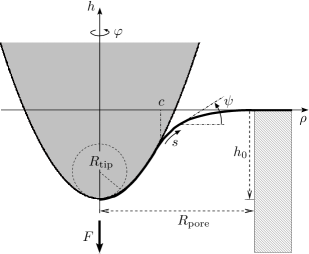
Figure 1: Illustration of the geometry. A parabolic tip with curvature radius $R_{\text{tip}}$ indents a pore-spanning membrane with a force $F$ to a certain depth $h_{0}$. The radius of the pore is $R_{\text{pore}}$. The membrane detaches from the tip at a radial distance $\rho=c$. The two possible parametrizations $h(\rho)$ and $\psi(s)$ are explained in the beginning of Chapter III.

The key “ingredient” underlying most of the new physics is the fact that the membrane can choose its point of detachment from the AFM tip. Unlike in the existing point force descriptions Goldstein02 ; Derenyi02 , in which a certain (pushing or pulling) force is applied at one point of the membrane, our description accounts for the fact that the generally nonvanishing interaction energy per unit area between tip and membrane co-determines their contact area over which they transmit forces, and thereby influence the entire force-distance-curve. What may at first seem like a minor modification of boundary conditions quickly proves to open a very rich and partly also complicated scenario, whose various facets may subsequently be used to extract information about the membrane. In fact, Smith et al. Smith03 ; Smith04 have demonstrated in a related situation that the competition between adhesion and tether pulling for substrate-bound vesicles gives rise to various first- and second-order transitions, details of which depend in a predictable way on the experimental setup. In our case we will for instance find snap-on and snap-off events between tip and membrane, which rest on the fact that binding is not pre-determined, and whose correct description is very important for reliably interpreting any AFM force experiments. Moreover, we will also see that the very occurrence of tethers is a much more subtle phenomenon, since an adhering membrane pulled upwards may in fact prefer to detach rather than being pulled into a tether—a question treated previously (and on the linear level) by Boulbitch Boulbitch .

Our paper is organized as follows: in Chapter II we introduce the model of our system and discuss the relevant energies. In Chapter III we present the equations that have to be solved in order to find membrane profiles, force-indentation curves and detachment forces. This will also include a treatment of the nonlinear case which was only mentioned very briefly in Ref. Steltenkamp_etal06 . In Chapter IV the results of our calculations are summarized and compared to existing Steltenkamp_etal06 measurements. We end in Chapter V with a discussion how the predictions for indentation and adhesion characteristics can be used to extract material properties in future experiments.

II The model

II.1 Geometry of the system

We consider a flat solid substrate with a circular pore of radius $R_{\text{pore}}$. A lipid bilayer membrane is adsorbed onto the substrate and spans the pore. In the situation we want to analyze an AFM tip is used to probe the properties of the free pore-spanning membrane. We assume that the tip has a parabolic shape with curvature radius $R_{\text{tip}}$ at its apex. Furthermore, we restrict ourselves to the static axisymmetric situation in which the tip pokes the free-standing membrane exactly in the middle of the pore (see Fig. 1).

For a certain downward force $F>0$ the membrane is indented to a corresponding depth $h_{0}>0$ which is measured from the plane of the substrate to the depth of the apex of the tip. Note that it is also possible to pull the membrane up with a force $F<0$ in the opposite direction if attractive interactions attach the membrane to the tip.

In the following, we will model the bilayer as a two-dimensional surface. This is a valid approach provided the thickness of the membrane (approx. 5 nm) is much smaller than (i) the membrane’s lateral extension as well as (ii) length scales of interest such as local radii of curvature.

With this geometric setup in mind, let us now consider the different energy contributions we want to include in our model.

II.2 Energy considerations

The total energy of the system “pore-tip” comprises different contributions: the membrane is under a lateral tension $\sigma$. To pull excess area into the pore, work has to be done against the adhesion between membrane and flat substrate substrate . It is given by $\sigma$ times the excess area lateraltension . Additionally, a curvature energy is associated with the membrane. According to Canham Canham70 and Helfrich Helfrich73 the Hamiltonian for an up-down symmetric membrane is then

$$E_{\text{elast}}=\int_{\Sigma}\!\!{\operatorname{d}}A\;\big{(}\sigma+\frac{\kappa}{2}K^{2}+\bar{\kappa}K_{\text{G}}\big{)}\;,$$ (1)

where $\Sigma$ denotes the surface of the membrane part which spans the pore. The proportionality constants $\kappa$ and $\bar{\kappa}$ are called bending rigidity and saddle-splay modulus, respectively. The Gaussian curvature $K_{\text{G}}$ is the product of the two principal curvatures whereas $K$ is their sum DifferentialGeometry ; signconvention . Note that the last term of energy (1) yields zero in our specific problem Gaussiancurvature .

With the help of the two material constants $\sigma$ and $\kappa$ one can define a characteristic lengthscale

$$\lambda:=\sqrt{\frac{\kappa}{\sigma}}\;,$$ (2)

which does not depend on geometric boundary conditions such as the radius of the tip or the pore but only on properties of the membrane. On scales larger than $\lambda$ tension is the more important energy contributions; on smaller scales bending dominates.

Apart from tension and bending, an adhesion between tip and membrane may contribute to the total energy. We assume that it is proportional to the contact area $A_{\text{contact}}$ between tip and membrane with a proportionality constant $w$, the adhesion energy per area.

If the indentation $h_{0}$ is given and one wants to determine the force $F$, the total energy can thus be written as

$$E^{h_{0}}_{\text{total}}=\int_{\Sigma}\!\!{\operatorname{d}}A\;\big{(}\sigma+\frac{\kappa}{2}K^{2}\big{)}-wA_{\text{contact}}\ .$$ (3)

Under certain circumstances, however, it is more convenient to consider the problem for a given force $F$. Both ensembles (“constant indentation” vs. “constant force”) are connected via a Legendre transformation Smith03 ; Smith04 , $E^{F}_{\text{total}}=E^{h_{0}}_{\text{total}}-Fh_{0}$. While the ground states one obtains for the two ensembles will be the same, questions of stability depend on the ensemble: a profile found to be stable under constant height conditions is not necessarily stable under constant force conditions.

The route we want to follow here in order to find force-indentation curves is to determine the equilibrium shapes of the non-bound section of the membrane via a functional minimization. The energy contributions caused by the bounded section of the membrane enter via the appropriate boundary conditions (see Chapter III and Appendix A). These imply that the contact point $c$ is not known a priori but has to be determined as well (“moving boundary problem”). In the next section we will show how one can set up the appropriate mathematical formulation of the problem to get membrane profiles and force-indentation curves.

III Shape equation and appropriate boundary conditions

To describe the shape of the membrane we use two different kinds of parametrization (see Fig. 1): for the linear approximation it is sufficient to use “Monge” gauge where the position of the membrane is given by a height $h(\rho)$ above (or below) the underlying reference plane. The disadvantage of this parametrization is that it does not allow for “overhangs”. Since these may be present in the full nonlinear problem, we will use the “angle-arclength” parametrization in the exact calculations: the angle $\psi(s)$ with respect to the horizontal substrate as a function of arclength $s$ fully describes the shape.

III.1 Linear approximations

To get the profile of the free membrane one has to solve the appropriate Euler-Langrange (“shape”) equation. This equation is typically a fourth order nonlinear partial differential equation and thus in most cases impossible to solve analytically. One may, however, consider cases where the membrane is indented only a little and gradients are small. In that case one may linearize the energy functional. In the constant indentation ensemble one gets for the free part

$$E=\int_{\Sigma_{\text{free}}}\!\!\!\!{\operatorname{d}}A_{\|}\;\Big{[}\frac{\kappa}{2}({\boldsymbol{\nabla}}^{2}h)+\frac{\sigma}{2}({\boldsymbol{\nabla}}h)^{2}\Big{]}\;,$$ (4)

where ${\operatorname{d}}A_{\|}$ is the area element on the flat reference plane and $\Sigma_{\text{free}}$ is the projected surface of the free pore-spanning membrane. The symbol ${\boldsymbol{\nabla}}$ denotes the two-dimensional nabla operator in the reference plane.

The appropriate shape equation can be derived by setting the first variation of energy (4) to zero, yielding

$${\boldsymbol{\nabla}}^{2}\big{(}{\boldsymbol{\nabla}}^{2}-\lambda^{-2}\big{)}h=0\;.$$ (5)

The solution to this equation is a linear combination of the eigenfunctions of the Laplacian corresponding to the eigenvalues 0 and $\lambda^{-2}$. For axial symmetry it is given by $h(\rho)=h_{1}+h_{2}\ln{(\rho/\lambda)}+h_{3}I_{0}(\rho/\lambda)+h_{4}K_{0}(\rho/\lambda)$, where $I_{0}$ and $K_{0}$ are the modified Bessel functions of the first and the second kind, respectively Abramowitz . The constants $h_{1},\ldots,h_{4}$ are determined from the appropriate boundary conditions (see Appendix A):

$$h(R_{\text{pore}}) = 0\;,\quad h(c)=-h_{0}+\frac{c^{2}}{2R_{\text{tip}}}\;,$$ (6a)

$$h^{\prime}(R_{\text{pore}}) = 0\;,\quad h^{\prime}(c)=\frac{c}{R_{\text{tip}}}\;,$$ (6b)

$$\text{and}\quad h^{\prime\prime}(c) = \frac{1}{R_{\text{tip}}}-\sqrt{\frac{2w}{\kappa}}\;,$$ (6c)

where a dash denotes a derivative with respect to $\rho$. Even though the differential equation is of fourth order, five conditions are required due to its moving boundary nature, i. e., $c$ is to be determined from an adhesion balance—which is in fact the origin of the fifth condition (6c) (see Appendix A).

The solution of the boundary value problem (5,6) can be used in two ways to calculate the force for a prescribed indentation: first, one can insert the profile back into the functional (4) to obtain the energy of the equilibrium solution, which will then parametrically depend on the indentation $h_{0}$. Its derivative with respect to $h_{0}$ yields the force $F$. Second, one can also consider stresses: in analogy to elasticity theory LaLi_elast $F$ is given by the integral of the flux of surface stress surfacestresstensor through a closed contour around the tip.

The second approach is used in the present work; it has the advantage that the final expression for the force can be written in a closed form Steltenkamp_etal06 (see also Appendix B):

$$F=2\pi R_{\text{pore}}\times\kappa\,\frac{\partial K}{\partial\rho}\Big{|}_{\rho=R_{\text{pore}}}\ .$$ (7)

This equation is exact. Inserting the solution $h(\rho)$ of the boundary value problem (5,6) into (7) yields the value of the force in the linear regime.

A little warning might be due here: expression (7) is evaluated at the rim of the pore where the profile is flat even for high indentations. One might thus wonder whether inserting the small gradient solution would actually lead to an exact result. This is, however, not the case, because the membrane shape at the rim predicted by the linear calculation is not identical with the prediction from the full nonlinear theory—except for its flatness, which is enforced by the boundary conditions. There is no magical way to avoid solving the nonlinear shape equation if one wants the exact answer.

III.2 Complete nonlinear formulation

Let us now shift to the angle-arclength parametrization and consider the full nonlinear problem. In principle, the constant height ensemble could be used here as well. It is, however, technically much easier to fix $F$ instead in order to reduce the number of boundary conditions one has to fulfill at the rim of the pore (see below and Appendix C).

In this paragraph all variables with a tilde are scaled with $\pi\kappa$, i. e.: $\tilde{E}:=E/(\pi\kappa)$, $\tilde{F}:=F/(\pi\kappa)$, etc. The energy functional of the free membrane can then be written as Berndl91 ; Hamiltonian95 ; Seifert97 ; wrapping2 ; Smith03 :

$$\tilde{E} = \int_{\underline{s}}^{\bar{s}}{\operatorname{d}}s\;\tilde{L}=\int_{\underline{s}}^{\bar{s}}{\operatorname{d}}s\;\Big{\{}\rho\;\Big{(}\dot{\psi}+\frac{\sin{\psi}}{\rho}\Big{)}^{2}+\frac{2\rho}{\lambda^{2}}$$ (8)

$$\quad+\,\lambda_{\rho}(\dot{\rho}-\cos{\psi})+\lambda_{z}(\dot{z}-\sin{\psi})-\tilde{F}\dot{z}\Big{\}}\;,\;\;\;\;$$

where $\underline{s}$ is the arclength at the contact point $c$ and $\bar{s}$ the arclength at $R_{\text{pore}}$. The dot denotes the derivative with respect to $s$. The Langrange multiplier functions $\lambda_{\rho}$ and $\lambda_{z}$ ensure that the geometric conditions $\dot{\rho}=\cos{\psi}$ and $\dot{z}=\sin{\psi}$ are fulfilled everywhere.

In order to make the numerical integration easier let us rewrite the problem in a Hamiltonian formulation Berndl91 ; Hamiltonian95 ; wrapping2 ; Smith03 : the conjugate momenta are $p_{\psi}=\partial\tilde{L}/\partial\dot{\psi}=2\rho[\dot{\psi}+\sin(\psi)/\rho]$, $p_{\rho}=\partial\tilde{L}/\partial\dot{\rho}=\lambda_{\rho}$, and $p_{z}=\partial\tilde{L}/\partial\dot{z}=\lambda_{z}-\tilde{F}$. The (scaled) Hamiltonian is then given by

$$\tilde{H}\! = \!\dot{\psi}p_{\psi}+\dot{\rho}p_{\rho}+\dot{z}p_{z}-\tilde{L}$$ (9)

$$= \!\frac{p_{\psi}^{2}}{4\rho}-\frac{p_{\psi}\sin{\psi}}{\rho}-\frac{2\rho}{\lambda^{2}}+p_{\rho}\cos{\psi}+(p_{z}+\tilde{F})\sin{\psi}.\;\;\;\;\,$$

Note that $\tilde{H}$ is not explicitly dependent on $s$ and is thus a conserved quantity. Instead of one fourth order one then has six first order ordinary differential equations, the Hamilton equations:

$$\dot{\psi} \;= \frac{\partial\tilde{H}}{\partial p_{\psi}} \;=\;\frac{p_{\psi}}{2\rho}-\frac{\sin{\psi}}{\rho}$$ (10a)

$$\dot{\rho} \;= \frac{\partial\tilde{H}}{\partial p_{\rho}} \;=\;\cos{\psi}$$ (10b)

$$\dot{z} \;= \frac{\partial\tilde{H}}{\partial p_{z}} \;=\;\sin{\psi}$$ (10c)

$$\dot{p}_{\psi} \;= -\frac{\partial\tilde{H}}{\partial\psi} \;=\;\Big{[}\frac{p_{\psi}}{\rho}-(p_{z}+\tilde{F})\Big{]}\cos{\psi}+p_{\rho}\sin{\psi}$$ (10d)

$$\dot{p}_{\rho} \;= -\frac{\partial\tilde{H}}{\partial\rho} \;=\;\frac{p_{\psi}}{\rho}\Big{(}\frac{p_{\psi}}{4\rho}-\frac{\sin{\psi}}{\rho}\Big{)}+\frac{2}{\lambda^{2}}$$ (10e)

$$\dot{p}_{z} \;= -\frac{\partial\tilde{H}}{\partial z} \;=\;0\;.$$ (10f)

According to the last equation, $p_{z}$ has to be constant along the profile. Its value can be found by considering the integral over the flux of surface stress which has to equal the applied force. This implies that $p_{z}$ vanishes everywhere (see Appendix B).

Equations (10) can be solved numerically subject to the boundary conditions (see also Appendices A and C):

$$\psi(\bar{s}) = 0\;,\quad\psi(\underline{s})=\alpha\;,$$ (11a)

$$\dot{\psi}(\underline{s}) = \frac{(\cos{\alpha})^{3}}{R_{\text{tip}}}-\sqrt{\frac{2w}{\kappa}}\;,$$ (11b)

$$\text{and}\quad\tilde{H} = 0\;,$$ (11c)

where contact radius $c$ and contact angle $\alpha$ are connected via $c=R_{\text{tip}}\tan{\alpha}$. The solution to (10, 11) gives the indentation $h_{0}$ for some prescribed force $\tilde{F}$.

IV Results

This chapter will summarize the characteristic features of the solution to the boundary value problems (5, 6) and (10, 11). In addition, the theory will be shown to be in accord with available experimental results.

We will introduce some additional variable rescaling in order to make generalizations of the results easier: lengths will be scaled with $R_{\text{tip}}$. We also define

$$\tilde{\sigma}:=\frac{\sigma R_{\text{tip}}^{2}}{\kappa}\quad,\quad\tilde{w}:=\frac{2wR_{\text{tip}}^{2}}{\kappa}\quad\text{and}\quad\tilde{f}:=\frac{FR_{\text{tip}}}{\pi\kappa}\;.$$ (12)

In a typical experiment the curvature of the tip is of the order of ten nanometer (5–40 nm) and pore radii may lie between 30 and 200 nm personalcommStelt . The bending rigidity of a fluid membrane may vary between one and a hundred $k_{\text{B}}T$ bendingrigidityfluidmembrane . One expects a maximum surface tension of the order of a few mN/m, which is approximately the rupture tension for a fluid phospholipid bilayer surfacetension . A maximum value of the adhesion can be found by assuming that a few $k_{\text{B}}T$ per lipid is stored if membrane and tip are in contact. One arrives at $w_{\text{max}}\approx 10\,\text{mJ}/\text{m}^{2}$. For the continuum theory to be valid Eqns. (6c, 11b) imply that $\sqrt{2w_{\text{max}}/\kappa}\lesssim 1/d$, where $d\approx 5\,\text{nm}$ is the bilayer thickness. This estimate yields approx. the same maximum value for $w_{\text{max}}$ as before since $\kappa$ is at most 100 $k_{\text{B}}T$.

Thus, $\tilde{\sigma}$ and $\tilde{w}$ can in principal vary between 0 and $10^{3}$. Realistically, if we set $R_{\text{tip}}=10\;\text{nm}$ and consider a typical fluid phospholipid bilayer with $\kappa\simeq 20\,k_{\text{B}}T$, $\tilde{\sigma}$ and $\tilde{w}$ are of the order of 1. Furthermore, we will focus on a pore radius of $\tilde{R}_{\text{pore}}=3$ in the following.

In order to understand, how adhesion energy modifies the force-distance behavior, let us first briefly revisit the case where there is no adhesion between tip and membrane ($\tilde{w}=0$).

IV.1 No adhesion between tip and membrane

In Fig. 2 the shapes of the membrane for different values of indentation are presented in scaled units. The linear calculations are dotted whereas the exact result is plotted with solid lines. For small indentations the two solutions overlap; for increasing $\tilde{h}_{0}$, however, the deviations become larger just as one expects for a small gradient approximation (see also Ref. wrapping2 for another example). While the differences are noticeable, they appear fairly benign, such that one would maybe not expect big changes in the force-distance behavior. We will soon find out that these hopes will not be fulfilled.

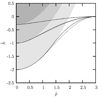
Figure 2: Membrane profiles for different indentations $\tilde{h}_{0}$, all for $\tilde{\sigma}=1$ (solid lines: nonlinear calulations, dashed lines: linear approximation, grey shades: AFM tips). The corresponding forces $\tilde{f}(\tilde{h}_{0})$ for the three different indentations are (nonlinear calculations): $\tilde{f}(0.3)=0.81$, $\tilde{f}(1)=2.45$, $\tilde{f}(2)=4.27$.

A deeper indentation also means that the tip has to exert a higher force. In Figs. 3 and 4 log-log plots of force-distance curves for different values of $\tilde{\sigma}$ are shown. The dashed line marks the maximum indentation $\tilde{h}_{0,\text{max}}=\tilde{R}_{\text{pore}}^{2}/2$ which is allowed by the geometry of tip and pore. In the limit of high forces all curves converge and approach $\tilde{h}_{0,\text{max}}$; for small forces the curves are linear in $\tilde{f}$. Let us quantify the indentation response by defining the (scaled) apparent spring constant $\tilde{\mathcal{K}}$ of the nanodrum-AFM system via

$$\tilde{\mathcal{K}}=\left.\frac{\partial\tilde{f}}{\partial\tilde{h_{0}}}\right|_{\tilde{w},\tilde{\sigma}}\ .$$ (13)

A linear force-distance-curve has a constant $\tilde{\mathcal{K}}$ and thus follows an apparent Hookean behavior $\tilde{f}=\tilde{\mathcal{K}}\tilde{h}_{0}$. In unscaled units, the spring constant is given by $\mathcal{K}=\partial F/\partial h_{0}=\tilde{\mathcal{K}}\pi\kappa/R_{\text{tip}}^{2}$. For typical values $R_{\text{tip}}=10\,\text{nm}$ and $\kappa=20\,k_{\text{B}}T$ this implies $\mathcal{K}=\tilde{\mathcal{K}}\times 2.6\,\text{mN/m}$.

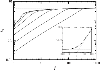
Figure 3: Force-distance curves for $\tilde{w}=0$ and $\tilde{\sigma}=\frac{1}{16},\frac{1}{4},1,4,16$ and $64$ ($\sigma$ increasing from left to right). The curve for $\tilde{\sigma}=0$ is dashed-dotted. The inset shows the corresponding scaled apparent spring constant $\tilde{\mathcal{K}}$ (see Eqn. (13)) in the small force limit, illustrating its two different regimes of small and large tension with a crossover around $\tilde{\sigma}\simeq 1$.

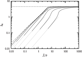
Figure 4: Scaled force-distance curves for $\tilde{w}=0$ and $\tilde{\sigma}=\frac{1}{16},\frac{1}{4},1,4,16$ and $64$ ($\sigma$ increasing from right to left). The solution for $\tilde{\sigma}\to\infty$ in the linear regime is dashed-dotted. Nonlinear results are plotted with solid lines, the linear approximation is dotted.

The smaller $\tilde{\sigma}$, the less force has to be applied to reach the same indentation (see Fig. 3). For decreasing $\tilde{\sigma}$ the force-distance curves converge to the limiting curve of the pure bending case, for which $\tilde{\sigma}=0$; this is plotted dashed-dotted in Fig. 3. In the opposite pure tension limit ($\kappa\rightarrow 0$ or $\tilde{\sigma}\to\infty$) the curves become essentially linear in $\tilde{\sigma}$, as can be seen clearly after scaling out the tension (see Fig. 4). It is possible to calculate this second limiting curve in the linear regime: the linearized Euler Lagrange equation reduces to the Laplace equation, $\Delta h=0$, which is solved by $h(\rho)=d_{1}+d_{2}\ln(\rho/R_{\text{pore}})$ in the present axial symmetry. The constants $d_{1}$ and $d_{2}$ can be determined with the help of the two boundary conditions $h(R_{\text{pore}})=0$ and $h(c)=-h_{0}+c^{2}/2R_{\text{tip}}$. The contact point $c$ is then determined by a straightforward energy minimization. The final result for the indentation depth is:

$$\tilde{h}_{0}^{\tilde{\sigma}\to\infty}=\frac{\tilde{f}/\tilde{\sigma}}{4}\bigg{[}1-\ln{\bigg{(}\frac{\tilde{f}/\tilde{\sigma}}{2\tilde{R}_{\text{pore}}^{2}}\bigg{)}}\bigg{]}\;,$$ (14)

which is plotted dashed-dotted in Fig. 4. At any given penetration the force is now strictly proportional to the tension. Notice also the remarkably weak (logarithmic) dependency of penetration on pore size.

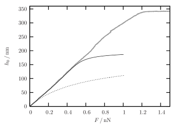
Figure 5: Comparison between experiment (solid grey line) and theory (dashed line: linear approximation; solid black line: nonlinear calculations) Steltenkamp_etal06 . The theoretical curves are obtained with the following parameters: $R_{\text{pore}}=90\,\text{nm}$, $R_{\text{tip}}=20\,\text{nm}$, $\kappa=10^{-19}\,\text{J}\approx 24\,k_{\text{B}}T$, $\sigma=1.1\,\text{mN/m}$.

All force-distance curves presented in this section exhibit a linear behavior for small forces. In this limit the scaled spring constant for the systems just discussed is well described by the empirical relation $\tilde{\mathcal{K}}\simeq 1.76+\tilde{\sigma}^{0.89}$ (see inset in Fig. 3). Combining this with our observation that for typical system parameters $\mathcal{K}=\tilde{\mathcal{K}}\times 2.6\,\text{mN/m}$, we see that a nanodrum’s stiffness can be very well matched by available (soft) AFM cantilevers, showing that the suggested experiments are indeed feasible. In fact, Fig. 5 shows the results of such an indentation experiment (solid grey line). Here, a fluid DOTAP (1,2-dioleoyl-3-trimethylammonium-propane chloride) membrane was suspended over a pore of radius $R_{\text{pore}}=90\,\text{nm}$ and subsequently probed with a tip of radius $R_{\text{tip}}=20\,\text{nm}$ Steltenkamp_etal06 . The apparent spring constant is found to be $3.9\,\text{mN/m}$. To fit the data we optimized the material parameters $\sigma$ and $\kappa$. The linear approximation (asymptotically) matches the curve down to an indentation depth of about 40 nm as one can see in Fig. 5 (dashed line). For larger indentations the small gradient assumption breaks down. The nonlinear calculation (solid black line) describes the data correctly down to a much deeper penetration depth of 150 nm but diverges for larger values. This deviation is most likely not a failure of the elastic model but a consequence of our simplified assumptions for the tip geometry. As shown in Fig. 1B of the Supplementary Information to Ref. Steltenkamp_etal06 the tip is parabolic at its apex, but further up it narrows quicker and assumes a more cylindrical shape. It therefore can penetrate the pore much deeper than one would expect if the parabolic shape were correct for the entire tip.

Apart from this difficulty, theory and experiment are in good agreement. There is, however, a catch. Since we cannot trust the force-distance behavior close to the depth-saturation (due to its displeasingly strong dependence on the actual tip shape), the remaining interpretable part of the force-distance-curve is linear, and its slope is the only parameter that can be extracted from the data axisintercept . For the theoretical calculation one needs two parameters, $\sigma$ and $\kappa$. Fitting both to a line is not possible. In Ref. Steltenkamp_etal06 this obstacle was overcome by estimating $\kappa$ from other measurements to be about $10^{-19}\,\text{J}$. The surface tension $\sigma$ could then be adjusted to $1.1\,\text{mN/m}$ to match the data—which, reassuringly, is a very meaningful value.

Alternatively, one may proceed in a different manner. In the experiment a small snap-off peak could be observed upon retraction of the AFM tip which was due to the attraction between tip and membrane. Although this could be neglected in the interpretation of the measurements of Ref. Steltenkamp_etal06 , one may think of deliberately increasing the adhesion between membrane and tip in a follow-up experiment by chemically functionalizing the tip. With this additional tuning parameter one may get further information on the values of the material parameters in question.

IV.2 Including adhesion between tip and membrane

In the following, we will also allow for adhesion between tip and membrane, i. e. $\tilde{w}$ is not necessarily equal to zero. This will change the qualitative behavior of the force-distance curves dramatically: for fixed $\tilde{\sigma}$ and $\tilde{w}$ different solution branches can be found. A hysteresis may occur as well, as we will see in the next section. Additionally, stable membrane profiles exist even if the tip is pulled upwards. It is therefore possible to calculate the maximum pulling force that can be applied before the tip detaches from the membrane and relate it to the value of the adhesion between tip and membrane.

IV.2.1 Weak adhesion energy

In this section, we will first investigate the case of weak adhesion, $\tilde{w}\leq 5$. The scaled surface tension $\tilde{\sigma}$ will be fixed to 1. It turns out that once the tip is adhesive, “overhang” profiles may occur, i. e., shapes where at some point $|\psi(s)|>90^{\circ}$. We will first ignore these solution branches and come back to them later.

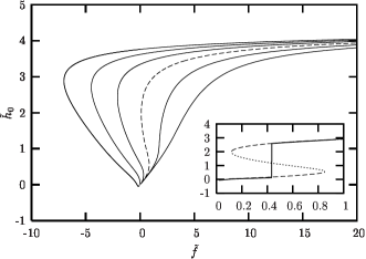
Figure 6: Force-distance curves for $\tilde{\sigma}=1$ and $\tilde{w}=0,1,2,3,4,5$ (from right to left). The region of hysteresis in the curve for $\tilde{w}=2$ is magnified in the inset. In this case the energy barrier at $\tilde{f}=0.414$ is approx. $1\,\kappa$. Overhang branches are omitted.

Fig. 6 illustrates force-distance-curves for $\tilde{w}=0,1,\ldots,5$. Compared to the nonadhesive case, for which an essentially linear behavior levels off towards maximum penetration, adhesive tips behave quite differently. Already for $\tilde{w}=1$ an initial Hookean response at small forces is soon followed by a regime in which the system displays a much greater sensitivity towards an externally applied stress, i. e., where the scaled spring constant $\tilde{\mathcal{K}}$ drops at intermediate penetrations. Physically this of course originates from the fact that adhesion helps to achieve higher penetrations, because the tip is pulled towards the membrane, but notice that this does not lead to a uniform reduction of $\tilde{\mathcal{K}}$: softening only sets in beyond a certain indentation.

Shortly beyond $\tilde{w}=1$ a point is reached where the force-distance-curve displays a vertical slope at which the apparent spring constant $\tilde{\mathcal{K}}$ vanishes. For even larger values of adhesion a hysteresis loop opens, featuring a locally unstable region with $\tilde{\mathcal{K}}<0$. This is the case for $\tilde{w}=2$, and the region around the instability is magnified in the inset of Fig. 6. Notice that the dotted branch corresponding to $\tilde{\mathcal{K}}<0$ still belongs to solutions for which the functional (3) is stationary, yet the energy plotted against penetration $\tilde{h}_{0}$ (or, alternatively, contact angle $\alpha$) has a local maximum, confirming that these solutions are unstable against contact point variations. The two dashed branches in the inset of Fig. 6 have a positive $\tilde{\mathcal{K}}$ and correspond to local minima in the energy, however, they are globally unstable against the alternative minimum of larger or smaller $\tilde{h}_{0}$. The true global minimum is indicated by the bold solid curve, which exhibits a discontinuity at $\tilde{f}=0.414$.

Depending on the current scanning direction this hysteretic force-distance-curve manifests itself in a snap-on or snap-off event. Such a behavior is reminiscent of a buckling transition (such as for instance Euler buckling of a rod under compression LaLi_elast )—with two caveats: first, notice that the membrane does not stay flat up to a critical buckling force at which it suddenly yields; rather, the system starts off with a linear stress-strain relation and only later undergoes an adhesion-driven discontinuity. Appreciating this point is quite important for the interpretation of measured force-distance curves: upon approach of tip and membrane the snap-on will occur neither at zero force nor at zero penetration. Second, one should not forget that hysteresis is ultimately a consequence of the energy barrier which goes along with such discontinuities. For macroscopic systems this barrier is typically so big that the transition actually happens at either of the two end-points of the S-shaped hysteresis curve, where the barrier vanishes (the “spinodal points”). However, for nano-systems barriers are much smaller, comparable to thermal energy $k_{\text{B}}T$, such that thermal fluctuations can assist the barrier-crossing event. In the present case the barrier at the equilibrium transition point is about $1\,\kappa$, i. e., about $20\,k_{\text{B}}T$ for typical bilayers. However, already at $\tilde{f}=0.5$ its magnitude has decreased by about 20%. This shows that we have to expect a narrowing-down of the hysteresis amplitude compared to an athermal buckling scenario.

Upon increasing the adhesion $\tilde{w}$ even further, one will reach a critical value $\tilde{w}_{0}$ at which the “back-bending branch” of the force-distance-curve touches the vertical line $\tilde{f}=0$. At this point the tip is being pulled into the pore even if there is no force at all. Conversely, neglecting barrier complications, this also implies that at the critical adhesion energy $\tilde{w}=\tilde{w}_{0}$ an infinitesimal pulling force will suffice to unbind tip and membrane, even though the adhesion between tip and membrane is greater than zero. It is very important to keep this fact in mind if one wants to use AFM measurements for the determination of adhesion energies.

For $\tilde{w}>\tilde{w}_{0}$ one obtains stable solutions even when pulling the tip upwards (where $\tilde{f}<0$) ftildele0 . The maximum possible force before detachment, $\tilde{f}_{\text{det}}$, again corresponds to the leftmost point of the back-bend, and it increases with increasing $\tilde{w}$; we will come back to this later. Notice that detachment always happens for values of $\tilde{h}_{0}$ which are positive, i. e., when the AFM tip is still below the substrate level. Contrary to what one might have expected, pulling will in this case not draw the membrane upwards into a tubular lipid bilayer structure (a “tether”), which at some specific elongation will fall off from the tip and snap back. Rather, the strong adhesion pulls the tip far into the pore, and while pulling on it indeed lifts it up, unbinding still happens below pore rim level.

IV.2.2 Strong adhesion energy

At even larger adhesion energy entirely new stationary solution branches emerge, as Fig. 7 illustrates for $\tilde{w}\in\{5,10,15\}$ and $\tilde{\sigma}=1$. We first recognize the well-known hysteretic branch, already seen in Fig. 6, which for increasing $\tilde{w}$ extends to much larger negative forces, even though the snap-off height $\tilde{h}_{0}$ does only change marginally. The shapes of two typical profiles are illustrated in the insets a and b. Notice that this branch is always connected to the origin, but for larger values of $\tilde{w}$ it starts off into the third quadrant (negative values for $\tilde{f}$ and $\tilde{h}_{0}$). At first sight it seems that we finally get solutions which correspond to a pulled-up membrane; however, this region close to the origin corresponds to a maximum and is thus unstable.

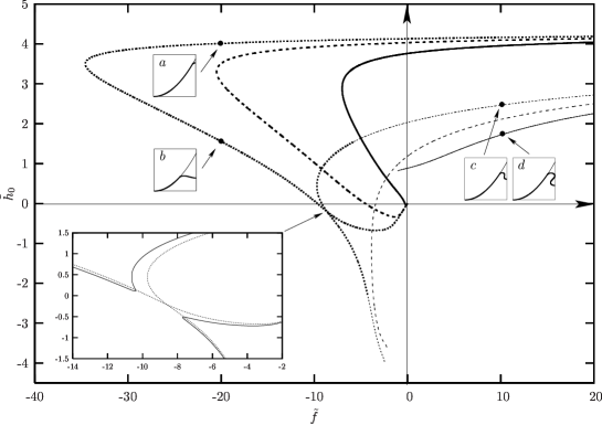
Figure 7: Force-distance curves for $\tilde{\sigma}=1$ and $\tilde{w}=5$ (solid), 10 (dashed) and 15 (dotted). A thinner line style is used for those parts of the curves where the corresponding profiles exhibit overhangs. In the insets a–d profiles for different values of $(\tilde{f},\tilde{h}_{0})$ are depicted (scaling is $\tilde{h}:\tilde{\rho}=5:3$). In the inset on the lower left corner the “branch splitting” is shown as discussed in the text ($\tilde{w}=15.0$ (dotted line) and $15.5$ (solid line)).

Overhang branches.

Contrary to the hysteretic branches, the new branches depicted in Fig. 7 do not connect to the origin. This classifies them as a genuinely nonlinear phenomenon, since they cannot be obtained as a small perturbation around the state $\tilde{f}=\tilde{h}_{0}=0$. In the first quadrant ($\tilde{f},\tilde{h}_{0}>0$) they all correspond to profiles which show overhangs (see inset $c$ and $d$). These branches had been omitted in Fig. 6, since for weak adhesion they always correspond to maxima and are thus irrelevant. This changes for stronger adhesion, though, where they become stable in certain regions (for instance, inset $c$ is locally stable). The details by which this happens are complicated and will be discussed in more detail below.

Following the new branches to negative forces we see that the one for $\tilde{w}=15$ loses its overhang around $\tilde{f}\approx-6$. That this can happen continuously is not surprising, since within angle-arc-length parametrization there is nothing special about the point where $|\psi|=90^{\circ}$ (only the shooting method might use occurrences of $|\psi|>90^{\circ}$ as a potential termination criterion for integration).

Branch splitting.

We also see that (for sufficiently large $\tilde{w}$) there is a point where the hysteresis branch intersects the new nonlinear branch. There the values of $\tilde{f}$ and $\tilde{h}_{0}$ coincide for both branches, but the detachment angle $\alpha$ and the total energy of the profile are generally different. However, the difference in energy at the intersection decreases with increasing $\tilde{w}$, and around $\tilde{w}=15.3$ it finally vanishes. At this degenerate point a branch splitting occurs, where the connectivity of the two branches re-bridges, as illustrated in the lower left inset in Fig. 7. Rather than connecting to the origin, the wide loop of the original hysteresis branch now joins into the overhang branch of the first quadrant, while its bit that was connected to the origin now joins into the overhang branch in the third quadrant.

Cusps.

Figure 8 shows the force-distance curve branches for the even larger adhesion energy $\tilde{w}=20$. This depicts a situation well after the branch-splitting, so we recognize the old hysteretic branch connecting with overhangs, and the branch connecting to the origin extending exclusively in the third quadrant. In contrast to Fig. 7, the line styles in Fig. 8 are chosen to illustrate local minima (solid) or maxima (dotted). What immediately strikes one as surprising is that the profiles at $\tilde{f}=-4$ belonging to the insets $f$ and $h$ both correspond to maxima, even though they sit on both sides of a back-bending branch, close to its end (compare this to the “usual” scenario at ($\tilde{f}\approx-49$, $\tilde{h}_{0}\approx 3.6$). Moreover, the solution belonging to inset $f$ turns into a local minimum for slightly more negative forces, without any noticeable features of the branch. How can this happen?

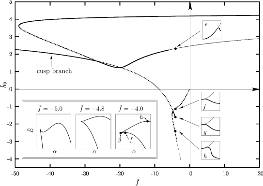
Figure 8: Force-distance curves for $\tilde{\sigma}=1$ and $\tilde{w}=20$ (including cusp branch). Solid lines correspond to local minima, dotted lines to local maxima. A thinner line style is used for those parts of the curves where the corresponding profiles exhibit overhangs. In the insets e - h profiles for different values of $(\tilde{f},\tilde{h}_{0})$ are depicted (scaling is $\tilde{h}:\tilde{\rho}=5:3$). In the inset on the left lower corner the total energy $\tilde{E}$ is plotted as a function of detachment angle $\alpha$ for different forces $\tilde{f}$ (see text for further explanation).

The explanation is illustrated in the lower left inset in Fig. 8, which shows the total energy as a function of detachment angle $\alpha$. Recall that extrema in this plot correspond to stationary solutions. As can be seen, the energy is multivalued, meaning that there exists more than one solution at a given detachment angle (these would then also differ in their value of their penetration $\tilde{h}_{0}$). But more excitingly, this graph exhibits a boundary extremum at a lowest possible nonzero value of $\alpha$ in the form of a cusp. This is how one can have two successive maxima on a curve without an intervening minimum—the minimum is simply not differentiable. Hence, there is a third solution branch, corresponding to the cusp, at which the contact curvature condition from Eqn. (11b) is not satisfied, because this condition is blind to the possibility of having non-differentiable extrema. Plotting this cusp branch also into Fig. 8, we finally understand how the switching of a maximum into a minimum happens: it occurs at the point of intersection with the cusp branch. As the lower left inset in Fig. 8 illustrates, the maximum belonging to the solution $f$ joins the cusp-minimum (belonging to solution $g$) in a boundary flat point, roughly at force $\tilde{f}=-4.8$. For more negative forces this flat point turns up, leaving a boundary cusp maximum and a new differentiable minimum. Notice that a similar exchange happens once more at ($\tilde{f}\approx-26.4$, $\tilde{h}_{0}\approx 1.6$). Incidentally, since at the cusp the contact curvature condition is not satisfied, and since this is the only point where the adhesion energy $\tilde{w}$ enters, the location and form of the cusp branch is independent of the value of $\tilde{w}$.

The existence of the cusp branch poses the question, whether the solutions corresponding to it are physically relevant (at least the ones which are minima). It is not so much the lack of differentiability at a cusp minimum which causes concern, but rather the fact that it is located at a boundary. Take for instance the $\tilde{E}(\alpha)$ curve in the lower left inset of Fig. 8 corresponding to $\tilde{f}=-4$. Now consider a (nonequilibrium) solution which sits on the upper branch, somewhere between the solutions $g$ and $h$. To lower the energy, this solution will reduce the detachment angle $\alpha$, thereby approaching the minimum at $g$. But once $g$ has been reached, no further reduction in $\alpha$ seems possible, since for smaller values no equilibrium solution exists. The crucial point is that our present theory is insufficient to answer what else would be going on for smaller $\alpha$. It could for instance be that there are indeed solutions, but they are not time-independent. This might be analogous to the well-known situation of a soap film spanned in the form of a catenoidal minimal surface between two coaxial circular rings of equal radius $R$. It is easy to show that for a ring separation exceeding $1.325\,R$ no more stationary solution exists, even though the limiting profile is in no way singular Arfken . However, when slowly pulling the two rings beyond this critical separation, the soap film does not suddenly rupture. Rather, it becomes dynamically unstable and begins to collapse. In the case we are studying here, the system drives itself to the singular boundary point, and without a truly dynamical treatment it is not possible to conclude whether it would remain there or start to dynamically approach a different solution. For this reason we do not want to overrate the significance of the cusp branch; yet, its existence is still important in order to explain the behavior of the other “regular” branches, for instance their metamorphosis from maximum-branches into minimum-branches or vice versa.

Detachment forces.

A measurable quantity in the experiment is the detachment force between tip and membrane, which is the maximum applicable pulling force $\tilde{f}_{\text{det}}$ before the tip detaches from the membrane. In Fig. 9 this force is plotted as a function of adhesion energy $\tilde{w}$ for different values of the scaled tension $\tilde{\sigma}$. Starting from a certain threshold adhesion $\tilde{w}_{\text{thr}}(\tilde{\sigma})$, below which no hysteresis occurs, $\tilde{f}_{\text{det}}$ decreases with increasing $\tilde{w}$ and exhibits a linear behavior for higher adhesions. Increasing $\tilde{\sigma}$ also increases the threshold adhesion (e. g. $\tilde{w}_{\text{thr}}(1/16)=0.22$ compared to $\tilde{w}_{\text{thr}}(1)=1.25$). In the large-$\tilde{w}$-limit $\tilde{f}_{\text{det}}/\tilde{w}=F_{\text{det}}/2\pi Rw$ finally approaches a limit which is independent of $\kappa$ and $\sigma$ and only depends on the geometry. The elasticity of the membrane no longer influences the measurement of the adhesion energy – not because the membrane is not deformed, but rather because its deformation energy is subdominant to adhesion. But for more realistic smaller values of $\tilde{w}$ this decoupling does not happen, and adhesion energies can only be inferred from the detachment force when a full profile calculation is performed.

At higher values of $\tilde{\sigma}$ also other qualitative features (such as additional instabilities) occur. However, these ramifications will not be discussed in the present work.

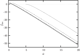
Figure 9: Scaled detachment force $\tilde{f}_{\text{det}}$ as a function of scaled adhesion energy $\tilde{w}$ for four values of the scaled tension, $\tilde{\sigma}=\frac{1}{16}$, $\frac{1}{4}$, $1$ and $4$ ($\tilde{\sigma}$ increasing from left to right).

Tethers.

Characteristically, the detachment happens at deep indentations ($\tilde{h}_{0}$ close to the maximum indentation possible). Long pulled-out membrane tubes (“tethers”), as they have been studied in the literature Goldstein02 ; Derenyi02 ; Koster05 , are not observed. Even though in our calculations we find profiles with $\tilde{h}_{0}<0$, these solutions either correspond to energetic maxima, or they are only local minima – with the global minimum at $\tilde{h}_{0}>0$ corresponding to a significantly lower energy. This is a consequence of the adhesion balance present in our situation: upon pulling upwards, it is more favorable for the tip either to be “sucked in” completely or to detach from the membrane, rather than forming a long tether. As Fig. 8 shows, there is a very small “window of opportunity” at $\tilde{f}\approx-5$ where (locally) stable solutions pulled above the surface exist. Yet, their profiles look essentially like the ones of inset $f$ or $g$ and show no resemblance to real long tethers. Upon increasing the force they become unstable, such that the tip either falls of the membrane, or is drawn below the membrane plane (notice that there exist two minima at $\tilde{f}$ slightly smaller than $-5$, but both at positive indentation).

This analysis shows that it appears impossible to pull tethers using a probe with a certain binding energy, despite existing experiments in which tethers of micrometer size were generated DaiShe95_99 ; MaeSenMeg02 ; Koster05 . Consequently, the assumption of an adhesion balance does not seem to be correct in these cases. Indeed, in these studies the experimental setup was different (membrane-covered micron-sized beads DaiShe95_99 ; Koster05 and AFM tips covered by lipid multilayers MaeSenMeg02 ). In the present situation tethers are also observed Steltenkamp_etal06 , but these events are not very reproducible, and based on the above calculations we would tentatively attribute them to a pinning of the membrane at some irregularity of the tip.

V Discussion

In the previous sections we have discussed the indentation of a pore-spanning bilayer by an AFM tip. We have seen that the force-distance curves show a linear behavior for small forces in a broad parameter range if the adhesion between tip and membrane vanishes. Even though this is in agreement with recent experiments (Steltenkamp_etal06 , see also Fig. 5), such a linear behavior is unfortunately too featureless to reveal the values of both elastic material constants, $\sigma$ and $\kappa$.

One way out of this apparent cul-de-sac would be to repeat the experiment for different pore radii $R_{\text{pore}}$ while keeping all other parameters fixed. Since $\sigma$ and $\kappa$ are the same for all pore sizes in that case, it should be possible to extract their value from the measured force-distance curves. Note that one does not have to fit both parameters simultaneously if one at first considers a pore where the radius is much larger than the characteristic lengthscale $\lambda$ (see Eqn. (2)). The corresponding system is in the high tension regime and the force-distance relation only depends on the surface tension (see Section IV.1). After determining $\sigma$ from the resulting curve, one may subsequently extract the value of $\kappa$ from a measurement of a system with smaller pore size.

The elastic constants can also be obtained by considering systems where the adhesion $w$ between tip and membrane has been increased experimentally. As we have seen, the curves change their behavior dramatically for $w\neq 0$. It should thus be possible to fit two parameters to the resulting curves which would yield a local $\kappa$ and $\sigma$ in one fell swoop whereas $w$ can simultaneously be determined from the snap-on of the tip upon approach to the bilayer. The experimentalist, however, has to make sure in that case that the line of contact between tip and membrane is really due to a force balance as described in this paper and not due to other effects such as pinning of the membrane to single spots on the tip. In practice, this is rather difficult and will be a challenge for future experiments.

One also has to keep in mind that the assumption of a perfect parabolic tip is quite simplistic compared to the experimental situation. It is probably valid in the vicinity of the apex but generally fails further up. Since the force-distance behavior close to the depth-saturation depends strongly on the actual tip shape, one can only use that part of the force-distance curve for data interpretation where the indentation is still small. To predict the whole behavior the exact indenter shape has to be known: as long as the situation stays axisymmetric one may, in principle, redo the calcutions of this publication with the new shape. This is, however, rather tedious and therefore inexpedient in practice.

Our theorical approach does not account for hydrodynamic effects although the whole setup is in water and the AFM tip is moved with a certain velocity. First measurements have shown, however, that it is possible to increase the velocity of the tip up to 60 $\mu\text{m}\,$$\text{s}^{-1}$ without altering the force-distance curves dramatically Steltenkamp_etal06 . One can understand this result with the help of the following simple estimate: assume that the tip is a sphere of radius $R_{\text{tip}}$ moving with the velocity $v$ in water. When indenting the membrane to a distance $d$ it will also have to overcome a dissipative hydrodynamic force $F_{\text{diss}}$ in addition to the elastic resistance of the membrane. The energy dissipated in this process, $E_{\text{diss}}=F_{\text{diss}}d=6\pi\eta R_{\text{tip}}vd$, is of the order of the thermal energy if typical values are inserted ($\eta=10^{-3}\text{Pa s}$, $R_{\text{tip}}=10\,\text{nm}$, $v=$ 60 $\mu\text{m}\,$$\text{s}^{-1}$, $d=100\,\text{nm}$). This is substantially smaller than the corresponding elastic energy $E_{\text{elast}}$. Complications arising from a correct hydrodynamical treatment were thus omitted here.

Including adhesion, the velocity of the measurement should nevertheless be as slow as possible to ensure that the line of contact equilibrates due to the force balance. If this is guaranteed, one can also check whether the predicted linear behavior between detachment force and adhesion is actually valid.

Appendix A Boundary conditions

In this appendix we will explain the origin of the boundary conditions (6) and (11): Eqns. (6a) follow simply from the requirement of continuity at the pore rim and the point where the membrane leaves the tip. Asking for a membrane that has no kinks and thus no diverging bending energy gives Eqns. (6b) and (11a).

If the membrane is free to choose its point of detachment as it is assumed here, an adhesion balance at the tip yields another boundary condition for the contact curvatures (6c/11b) (see (LaLi_elast, , Sec. 12, problem 6), Seifert90 , and wrapping2 ). In Ref. wrapping2 a quick derivation can be found for the axisymmetric case in the constant height ensemble: varying the point of contact changes the energy of the free profile but also the energy due to the part at the tip. By setting the total variation to zero one obtains the well-known contact curvature condition (Eqn. (6c) in Monge gauge). Observe that this assumes differentiability of the energy as a function of contact point position. In the force ensemble an extra term $\tilde{F}\delta h$ has to be added to the variation of the bound membrane. A term that is equal and opposite, however, enters the variation of the free membrane via the Hamiltonian (9). In total, both terms cancel and one again obtains the same condition (Eqn. (11b) in angle-arclength parametrization).

The remaining condition (11c) stems from the fact that the total arclength is not a conserved quantity, which it would be if we used a fixed interval of integration. Relaxing this unphysical constraint requires the Hamiltonian to vanish Hamiltonian95 ; CastroVillarealGuven06 .

Appendix B Calculation of the force via the stress tensor

If the shape of the free membrane is known, the stress tensor ${\boldsymbol{f}}^{a}$ ($a\in\{1,2\}$) can be evaluated at every point of the surface $\Sigma_{\text{free}}$. The integral of its flux through an arbitrary contour $\gamma$ which encloses the tip gives the force surfacestresstensor

$$F=-{\boldsymbol{e}}_{h}\cdot\oint_{\gamma}{\operatorname{d}}s\,\Big{\{}\Big{[}\frac{\kappa}{2}(K_{\perp}^{2}-K_{\|}^{2})-\sigma\Big{]}\,{\boldsymbol{l}}-\kappa(\nabla_{\perp}K)\,{\boldsymbol{n}}\Big{\}}\;.$$ (15)

The normal vectors ${\boldsymbol{l}}$ and ${\boldsymbol{n}}$ are perpendicular to $\gamma$ and to each other in every point of the curve. In addition, ${\boldsymbol{l}}$ is tangential to the surface whereas ${\boldsymbol{n}}$ is normal to it. $K_{\perp}$ and $K_{\|}$ are the curvatures perpendicular (in direction of ${\boldsymbol{l}}$) and tangential to the curve. The symbol $\nabla_{\perp}$ denotes the derivative along ${\boldsymbol{l}}$.

In angle-arclength parametrization, the curvatures are given by: $K_{\perp}=-\dot{\psi}$, $K_{\|}=-\sin{(\psi)}/\rho$, and $K=-p_{\psi}/(2\rho)$. Eqn. (15) can then be written as

$$F = -\frac{\kappa}{2}\oint_{\gamma}{\operatorname{d}}s\;\Big{\{}\Big{[}\Big{(}\dot{\psi}^{2}-\frac{\sin^{2}{\psi}}{\rho^{2}}\Big{)}-\sigma\Big{]}\sin{\psi}$$ (16)

$$\qquad\qquad\quad+\;\frac{1}{\rho}\Big{(}\dot{p}_{\psi}-\frac{p_{\psi}}{\rho}\dot{\rho}\Big{)}\cos{\psi}\Big{\}}\;.$$

The integrand can be evaluated further by inserting the Hamilton equations (10) and making use of the fact that the Hamiltonian (9) is zero. One obtains

$$F=\frac{\kappa}{2}\oint_{\gamma}{\operatorname{d}}s\;\Big{(}\frac{p_{z}+\tilde{F}}{\rho}\Big{)}\;.$$ (17)

If we now exploit axial symmetry by integrating around a circle of radius $\rho=R_{\text{int}}$, we finally get $F=p_{z}+F$; the momentum $p_{z}$ conjugate to $z$ has to vanish identically which implies that the Lagrange multiplier function $\lambda_{z}$ is equal to $\tilde{F}$. This at first maybe surprising result is no coincidence at all. In fact, in Ref. CastroVillarealGuven06 it was shown that the Lagrange multiplier functions which fix the geometrical constraints are closely related to the external forces via the conservation of stresses.

Expression (15) can also be translated into “Monge gauge”. If we again exploit axial symmetry and integrate around a circle of radius $\rho=R_{\text{int}}$, it reads

$$F = -2\pi R_{\text{int}}\Bigg{\{}\Big{[}\frac{\kappa}{2}\Big{(}\frac{h^{\prime\prime}(\rho)^{2}}{g^{3}}-\frac{h^{\prime}(\rho)^{2}}{\rho^{2}g}\Big{)}-\sigma\Big{]}\frac{h^{\prime}(\rho)}{\sqrt{g}}$$ (18)

$$\qquad\qquad+\;\kappa\Big{(}\frac{h^{\prime\prime}(\rho)}{\sqrt{g}^{3}}+\frac{h^{\prime}(\rho)}{\rho\sqrt{g}}\Big{)}^{\prime}\;\frac{1}{g}\Bigg{\}}\Bigg{|}_{\rho=R_{\text{int}}}\!\!,$$

where $g=1+h^{\prime}(\rho)^{2}$. Note that the dash denotes derivatives with respect to $\rho$.

If in particular we choose to evaluate the force at $R_{\text{int}}=R_{\text{pore}}$, the expression (18) simplifies considerably to Eqn. (7).

Appendix C Numerical calculations

The Hamilton equations (10) were solved by using a shooting method NumericalRecipes : for a trial contact point $c$ Eqns. (10) were integrated with a fourth-order Runge-Kutta method. The value of $c$ determined the contact angle $\alpha$ and with it $\psi$, $\rho$, $p_{\psi}$, and $p_{\rho}$ at $s=\underline{s}$ via the boundary conditions (11). The integration was stopped as soon as $\rho$ was equal or greater than $R_{\text{pore}}$. To reach $R_{\text{pore}}$ exactly one extra integration with the correct stepsize backwards was performed. Finally, the value(s) of $c$ for which $\psi=0$ at $R_{\text{pore}}$ were identified for fixed parameters $F$, $\sigma$, $w$, etc.

If the calculation had been done in the constant height ensemble, one would additionally have to check whether the correct indentation $h_{0}$ was reached at $\rho=R_{\text{pore}}$ after shooting. In the constant force ensemble this complication of meeting a second condition is avoided which is why we chose to use it for the nonlinear calculations.

References

- (1) H. Lodish, A. Berk, S. L. Zipursky, P. Matsudaira, D. Baltimore, and J. Darnell, Molecular Cell Biology (Freeman & Company, New York, 2000).
- (2) M. Marsh (ed.), Endocytosis, Frontiers in Molecular Biology, (Oxford University Press, Oxford, 2001).
- (3) T. Kirchhausen, Curr. Opinion Struc. Biol. 3, 182 (1993).
- (4) M. S. Robinson, Trends Cell Biol. 7, 99 (1997).
- (5) H. T. McMahon and J. L. Gallop, Nature 438, 590 (2005).
- (6) H. Garoff, R. Hewson und D.-J. E. Opstelten, Microbiol. Mol. Biol. Rev. 62, 1171 (1998).
- (7) E. J. Luna, A. L. Hitt, Science 258, 955 (1992).
- (8) M. Umeda and K. Emoto, Chem. Phys. Lipids 101, 81 (1999).
- (9) F. Brochard and J. F. Lennon, J. Phys. (Paris) 36, 1035 (1975).
- (10) J. F. Faucon, M. D. Mitov, P. Meleard, I. Bivas and P. Bothorel, J. Phys. (Paris) 50, 2389 (1989).
- (11) E. Evans and W. Rawicz, Phys. Rev. Lett. 64, 2094 (1990).
- (12) W. Rawicz, K. C. Olbrich, T. McIntosh, D. Needham, and E. Evans, Biophys. J. 79, 328 (2000).
- (13) J. Dai and M. P., Sheetz, Biophys. J. 68, 988 (1995); Biophys. J. 77, 3363 (1999).
- (14) R. M. Hochmuth, J. Y. Shao, J. Dai and M. P. Sheetz, Biophys. J. 70, 358 (1996).
- (15) D. Cuvelier, I. Derényi, P. Bassereau and P. Nassoy, Biophys. J. 88, 2714 (2005).
- (16) N. Maeda, T. J. Senden, and J.-M. di Meglio, BBA-Biomembranes 1564, 165 (2002).
- (17) S. R. Heidemann and D. Wirtz, Trends Cell Biol. 14, 160 (2004).
- (18) D. A. Brown and E. London, Biochemm Biophys. Res. Comm. 240, 1 (1997); Annu. Rev. Cell Develop. Biol. 14, 111 (1998).
- (19) K. Simons and E. Ikonen, Nature 387, 569 (1997).
- (20) S. Munro, Cell 115, 377 (2003).
- (21) B. Nichols, Nature 436, 638 (2005).
- (22) J. F. Hancock, Nature Rev. Mol. Cell Biol. 7, 456 (2006).
- (23) H.-J. Butt, B. Cappella and M. Kappl, Surf. Sci. Rep. 59, 1 (2005).
- (24) M. Radmacher, Methods in Cell Biol. 68, 67 (2002).
- (25) K. D. Kosta, Disease Markers 19, 139 (2003).
- (26) S. Steltenkamp, M. M. Müller, M. Deserno, C. Hennesthal, C. Steinem and A. Janshoff, Biophys. J. 91, 217 (2006).
- (27) P. B. Canham, J. Theoret. Biol. 26, 61 (1970).
- (28) W. Helfrich, Z. Naturforsch. 28c, 693 (1973).
- (29) T. R. Powers, G. Huber, and R. E. Goldstein, Phys. Rev. E 65, 041901 (2002);
- (30) I. Derényi, F. Jülicher, and J. Prost, Phys. Rev. Lett. 88, 238101 (2002).
- (31) S. Svetina and B. Žekš, Eur. Biophys. J. 17, 101 (1989);
- (32) L. Miao, B. Fourcade, M. Rao, M. Wortis, and R. K. P. Zia, Phys. Rev. A 43, 6843 (1991).
- (33) U. Seifert, K. Berndl, and R. Lipowsky, Phys. Rev. A 44, 1182 (1991).
- (34) F. Jülicher and U. Seifert, Phys. Rev. E 49, 4728 (1994).
- (35) U. Seifert, Adv. Phys. 46, 13 (1997).
- (36) U. Seifert and R. Lipowsky, Phys. Rev. A 42, 4768 (1990).
- (37) U. Seifert, Phys. Rev. Lett. 74, 005060 (1995).
- (38) M. Deserno and T. Bickel, Europhys. Lett. 62, 767 (2003).
- (39) M. Deserno, Phys. Rev. E 69, 031903 (2004).
- (40) M. Deserno, J. Phys.: Condens. Matter 16, S2061 (2004).
- (41) A.-S. Smith, E. Sackmann, and U. Seifert, Europhys. Lett. 64, 281 (2003).
- (42) A.-S. Smith, E. Sackmann, and U. Seifert, Phys. Rev. Lett. 92, 208101 (2004).
- (43) G. Koster, A. Cacciuto, I. Derényi, D. Frenkel, and M. Dogterom, Phys. Rev. Lett. 94, 068101 (2005).
- (44) A. Boulbitch, Europhys. Lett. 59, 910 (2002).
- (45) Note that the part of the system outside the pore just acts like a reservoir fixing the lateral tension. Its energetics do not have to be considered explicitly.
- (46) F. David and S. Leibler, J. Phys. II 1, 959 (1991).
- (47) M. Do Carmo, Differential Geometry of Curves and Surfaces, (Prentice Hall, 1976); E. Kreyszig, Differential Geometry, (Dover, New York, 1991).
- (48) The convention used in this article is that a sphere with outward pointing normal vector has a positive .
-
(49)
The Gauss-Bonnet theorem states that:
for a simply connected surface DifferentialGeometry . In our case the boundary of the surface is a circle of radius . Its geodesic curvature is equal to , such that the second integral yields . Thus, the integral over the Gaussian curvature is zero as long as no topological changes occur. - (50) Handbook of Mathematical Functions, 9th ed., edited by M. Abramowitz and I. A. Stegun (Dover, New York, 1970).
- (51) L. D. Landau and E. M. Lifshitz, Theory of Elasticity, 3rd ed. (Butterworth-Heinemann, Oxford, 1986).
- (52) R. Capovilla and J. Guven, J. Phys. A: Math. Gen. 35, 6233 (2002).
- (53) S. Steltenkamp, personal communication.
- (54) U. Seifert and R. Lipowsky, Morphology of vesicles; in Handbook of Biological Physics, vol. 1A, edited by R. Lipowsky and E. Sackmann (Elsevier, Amsterdam, 1995).
- (55) E. Evans, V. Heinrich, F. Ludwig, and W. Rawicz, Biophys. J. 85, 2342 (2003).
- (56) The axis intercept is needed to gauge the distance between AFM tip and substrate in the experiment and can therefore not be extracted as a second parameter.
- (57) Strictly speaking all of these solutions are metastable with respect to detachment of the tip from the membrane.
- (58) G.B. Arfken and H.J. Weber, Mathematical Methods for Physicists, 6th ed., (Elsevier, Amsterdam, 2005); Example 17.2.2.
- (59) P. Castro-Villarreal and J. Guven, arXiv:cond-mat/0608230 (2006).
- (60) Numerical Recipes in C, 2nd ed., edited by W.H. Press et al. (Cambridge University Press, Cambridge, 1992)