On the high density behavior of Hamming codes with fixed minimum distance

Abstract

We discuss the high density behavior of a system of hard spheres of diameter $d$ on the hypercubic lattice of dimension $n$, in the limit $n\rightarrow\infty$, $d\rightarrow\infty$, $d/n=\delta$. The problem is relevant for coding theory, and the best available bounds state that the maximum density of the system falls in the interval $1\leq\rho V_{d}\leq\exp(n\kappa(\delta))$, being $\kappa(\delta)>0$ and $V_{d}$ the volume of a sphere of radius $d$. We find a solution of the equations describing the liquid up to an exponentially large value of $\widetilde{\rho}=\rho V_{d}$, but we show that this solution gives a negative entropy for the liquid phase for $\widetilde{\rho}\gtrsim n$. We then conjecture that a phase transition towards a different phase might take place, and we discuss possible scenarios for this transition.

A code $C$ is a subset of the binary Hamming space $H_{2}^{n}=\{0,1\}^{n}$. The distance between two points $s,t\in H_{2}^{n}$ is the Hamming distance $d(s,t)=\sum_{\alpha=1}^{n}(s_{\alpha}+t_{\alpha})_{\text{mod}2}$, i.e. it is given by the number of different bits. We consider the problem of finding the maximal size $A(n,d)$ of a code $C$ such that the minimum distance between two points in $C$ is $d$, that means, denoting by $|C|$ the number of sequences in $C$,

$$A(n,d)=\max\Big{[}\,|C|\,\Big{|}\,\forall s,t\in C,\,d(s,t)\geq d\Big{]}\ .$$ (1)

In particular we are interested in the quantity

$$R(\delta)=\limsup_{n\rightarrow\infty,\,d/n\rightarrow\delta}\frac{1}{n}\log_{2}A(n,d)\ ,$$ (2)

where the supremum is taken on all possible sequences of codes such that $d/n\rightarrow\delta$. The problem trivializes for $\delta>1/2$ as the total number of sequences is finite and $R(\delta)=0$. An interesting scaling is $d/n=1/2-\varepsilon n^{-\alpha}$, as for an appropriate choice of $\alpha$ the number $A(n,d)$ might increase polynomially in $n$, but this will not be investigated here. Thus we will restrict to $\delta<1/2$ in the following.

This problem is relevant for the theory of error correcting codes VG ; PS99 ; MRRW77 ; BJ01 ; Sa01 ; De73 . In “physics language”, it is the problem of finding the maximum possible density of a system of hard spheres on the hypercubic lattice. This rephrasing of the problem has been shown to be useful as it allows to use well known methods borrowed from the theory of liquids, like the virial expansion PS99 .

In this paper we will discuss the behavior of the system at high density, in order to understand how one can try to compute the maximum density. We will show that, for large $n$, the problem closely resembles the problem of hard spheres in $\hbox{\msytw R}^{n}$ in the limit of large space dimension $n$. The basic idea is that in this limit the number of neighbors of a sphere is large, much as it happens in the continuum for large space dimension. We will then discuss some recent ideas that have been used in the continuum FP99 ; PS00 ; PZ06 ; To06 to make some progress in the direction of deriving bounds on $A(n,d)$.

The best known lower bound on $A(n,d)$ (Varshamov-Gilbert bound) states that the density $\rho=|C|/2^{n}\geq 1/V_{d-1}$, $V_{d}$ being the volume of a sphere of radius $d$ in $H_{2}^{n}$ VG . This bound can be proven from the convergence of the virial series PS99 and gives $R(\delta)\geq R_{VG}(\delta)=1-H(\delta)$, $H(\delta)$ being the binary entropy function (see below). This means that a “liquid phase”, defined by the virial equation of state, exists at least up to $\rho V_{d-1}\sim 1$. We will show that the liquid phase can be formally continued up to a density $\rho V_{d-1}\sim\exp(n\kappa(\delta))$ with $\kappa(\delta)>0$: this result correspond to the Frisch-Percus result in the continuum FP99 .

However, we find that the entropy of the liquid becomes negative at $\rho V_{d-1}\sim n$. This suggests the possible instability of the liquid towards a different phase, i.e. the existence of a phase transition. We will discuss two different possibilites. By analogy with the problem in $\hbox{\msytw R}^{n}$ for large $n$, we conjecture that a glass transition might be present also in this system. In absence of other phases (such as “crystalline” phases), this analogy suggests that $R(\delta)$ is given by the Varshamov-Gilbert result, $R(\delta)=R_{VG}(\delta)$. We will also discuss a different instability that happens for even $d$, leading to a first order transition to a phase where the particles move on a sublattice of $H^{n}_{2}$.

The calculation of the properties of the (eventual) glassy phase requires the use of the replica method, but this turns out to be more difficult than in $\hbox{\msytw R}^{n}$ so we leave it for future work.

The paper is organized as follows: in section I we set up the basic notations and definitions; in section II we review the known bounds on $R(\delta)$; in section III we present our main results and conjectures on the high density behavior of the system; finally in section IV we draw the conclusions and present a summary of our ideas.

I Hard spheres on the hypercube

I.1 Definitions

Let $s=(s_{1},\cdots,s_{n})$, $s_{\alpha}\in\{0,1\}$, be a point in $H^{n}_{2}$. We define the Hamming distance between two points

$$d(s,t)=\sum_{\alpha=1}^{n}(s_{\alpha}+t_{\alpha})_{\text{mod}2}\ .$$ (3)

The number of points at distance $i$ from the origin is $S_{i}\equiv\binom{n}{i}$ and the volume of a sphere of radius $d$ centered in the origin is

$$V_{d}\equiv\sum_{t:d(0,t)\leq d}1=\sum_{i=0}^{d}\binom{n}{i}\ .$$ (4)

The interaction potential between two particles in $s$ and $t$ is the hard core potential:

$$U(s,t)=\begin{cases}0\hskip 15.0ptd(s,t)\geq d\ ,\\ \infty\hskip 10.0ptd(s,t)<d\ .\end{cases}$$ (5)

The grancanonical partition function Hansen ; PS99 is

$${\cal Z}_{n}[z]=\sum_{N=0}^{2^{n}}\frac{z^{N}}{N!}\sum_{s_{1}\cdots s_{N}}e^{-\sum_{i<j}U(s_{i},s_{j})}\ ,$$ (6)

the average number of spheres (to be identified with the average size of the code, $|C|$) is $\left\langle N\right\rangle=z\frac{\partial\ln{\cal Z}_{n}}{\partial z}$ and $A(n,d)=\lim_{z\rightarrow\infty}\left\langle N\right\rangle$. The density is $\rho\equiv\left\langle N\right\rangle/2^{n}$ and it is convenient to define the reduced density

$$\widetilde{\rho}\equiv\rho V_{d-1}=\frac{\left\langle N\right\rangle V_{d-1}}{2^{n}}\ ,$$ (7)

and

$$\varphi=\frac{1}{n}\ln\widetilde{\rho}\ .$$ (8)

For $n\rightarrow\infty$ and $d/n=\delta<1/2$ one has

$$v(\delta)=\lim_{n\rightarrow\infty}\frac{1}{n}\ln V_{n\delta}=-\delta\ln\delta-(1-\delta)\ln(1-\delta)\ ,$$ (9)

i.e. $V_{d}\sim S_{d}=\binom{n}{d}\sim e^{nv(\delta)}$, so that

$$\varphi=\frac{1}{n}\ln\widetilde{\rho}\sim\frac{1}{n}\ln\rho+v(\delta)\ ,\hskip 10.0pt\rho\sim e^{n[\varphi-v(\delta)]}\ .$$ (10)

The pair distribution function is given by the average number of particle pairs such that one particle is in $s$ and the other in $t$ Hansen :

$$\rho_{2}(s,t)\equiv\left\langle\sum_{i\neq j}\delta_{s,s_{i}}\delta_{t,s_{j}}\right\rangle\equiv\rho^{2}g(d(s,t))$$ (11)

where the Kronecker $\delta_{s,t}$ is equal to one if $s=t$ and to zero otherwise. The pair distribution function $g(i)$ is normalized to have value $1$ at large distance (for $n\rightarrow\infty$). We also define $h(i)\equiv g(i)-1$ which vanishes at large distance. Note that the function $\rho g(d(0,s))$ is the probability of finding a particle in the point $s$, given that there is a particle in the origin.

I.2 Liquid phase

The liquid phase is defined by the virial expansion of the partition function at low densities which converges for $\rho V_{d-1}\leq 1/6e$ PS99 . However, one can try to perform a continuation of the liquid equation of state below the radius of convergence of the virial series. For hard spheres in $\hbox{\msytw R}^{3}$, such a continuation is possible: approximated expressions are usually obtained by resumming some class of diagrams of the virial expansion to get a closed integral equation for the pair correlation function $g(i)$. Well known resummations are the Percus-Yevick (PY) and the HyperNetted Chain (HNC) ones, and agree well with numerical results Hansen .

For hard spheres in $\hbox{\msytw R}^{n}$ it has been shown by Frisch and Percus FP99 that in the limit of large $n$ the virial series is dominated order by order by the so-called ring diagrams. The resummation of the ring diagrams has been shown to provide a reasonable analytic continuation of the liquid equation of state up to very large values of the density FP99 . As the latter diagrams are included in the HNC resummation, the two resummations should be equivalent in the large dimension limit. The advantage of the HNC resummation is that it leads to a closed expression for the free energy corresponding to the partition function (6) for any finite $n$. The HNC free energy (per particle) is:

$$\Psi[g]=\frac{\rho}{2}\sum_{i=0}^{n}S_{i}\big{[}g(i)\ln g(i)-g(i)+1\big{]}+\ln\rho-1+\frac{1}{2\,\rho\,2^{n}}\sum_{p\geq 3}\frac{(-1)^{p}\rho^{p}}{p}\text{Tr}h^{p}\ ,$$ (12)

where

$$\text{Tr}h^{p}=\sum_{s_{1}\cdots s_{p}}h(s_{1},s_{2})h(s_{2},s_{3})\cdots h(s_{p},s_{1})\ ,$$ (13)

and the function $g(i)$ is determined by the stationarity condition $\frac{\delta\Psi}{\delta g}=0$ (HNC equation). We will argue that a solution to the HNC equations (or to similar approximations to the equation of state of the liquid, that should be equivalent for $n\rightarrow\infty$) exists up to $\widetilde{\rho}\sim\exp(n\kappa)$ with $\kappa>0$, thus defining the continuation of the liquid equation of state in this region of densities.

I.3 Fourier transform

To write the last term of the HNC free energy in a more convenient way it is useful to define the Fourier transform on the hypercube. Define the scalar product of two sequences as $s\cdot t\equiv\sum_{\alpha=1}^{n}s_{\alpha}t_{\alpha}$ (such that $s^{2}\equiv s\cdot s=d(0,s)$) and let us indicate by $s+t$ the sum (modulo 2) of the two sequences. Then if $q\in\{0,1\}^{n}$ the Fourier transform of a function $h(s)$ is given by

$$\begin{split}\widehat{h}(q)&=\sum_{s}(-1)^{q\cdot s}h(s)\ ,\\ h(s)&=\frac{1}{2^{n}}\sum_{q}(-1)^{q\cdot s}\widehat{h}(q)\ ,\end{split}$$ (14)

Using the property $\sum_{s}(-1)^{(q_{1}+q_{2})\cdot s}=2^{n}\delta_{q_{1},q_{2}}$ the Fourier transform of a function $h(s,t)=h(s+t)$ is

$$\begin{split}&\sum_{s,t}(-1)^{q_{1}\cdot s}(-1)^{q_{2}\cdot t}h(s+t)=2^{n}\delta_{q_{1},q_{2}}\widehat{h}(q_{1})\ ,\\ &h(s,t)=\frac{1}{2^{n}}\sum_{q}(-1)^{q\cdot(s+t)}\widehat{h}(q)\ .\end{split}$$ (15)

Moreover if $h(s,t)=h(d(s,t))$ (a rotationally invariant function), its Fourier transform depends only on $a\equiv q^{2}=d(0,q)$, see Eq. (3), and one has

$$\begin{split}&\widehat{h}(a)=\sum_{i=0}^{n}{\cal F}_{n}(a,i)h(i)\ ,\\ &h(i)=\frac{1}{2^{n}}\sum_{a=0}^{n}{\cal F}_{n}(i,a)\widehat{h}(a)\ ,\\ &{\cal F}_{n}(a,i)=\sum_{s:d(0,s)=i}(-1)^{\sum_{\alpha=1}^{a}s_{\alpha}}=\sum_{m=\max(0,i+a-n)}^{\min(a,i)}(-1)^{m}\binom{a}{m}\binom{n-a}{i-m}=K_{i}(n,a)\ ,\end{split}$$ (16)

where $K_{i}(n,a)$ is a Krawtchouk polynomial Sa01 ; kraw . The matrix ${\cal F}_{n}(a,i)$ has the following symmetries that will be useful in the following:

$$\binom{n}{a}{\cal F}_{n}(a,i)=\binom{n}{i}{\cal F}_{n}(i,a)\ ,$$ (17)

$${\cal F}_{n}(n-a,i)=(-1)^{i}{\cal F}_{n}(a,i)\ ,$$ (18)

$${\cal F}_{n}(a,n-i)=(-1)^{a}{\cal F}_{n}(a,i)\ ,$$ (19)

$${\cal F}_{n}(n-a,n-i)=(-1)^{n-a-i}{\cal F}_{n}(a,i)\ .$$ (20)

It satisfies ${\cal F}_{n}(0,i)=\binom{n}{i}$ and ${\cal F}_{n}(a,0)=1$, and can be easily constructed using the recursion relations

$$\begin{split}&{\cal F}_{n+1}(a,0)=1\ ,\\ &{\cal F}_{n+1}(a,i+1)={\cal F}_{n}(a,i)+{\cal F}_{n}(a,i+1)\ ,\hskip 20.0pta\leq n\ ,\\ &{\cal F}_{n+1}(n+1,i+1)=-{\cal F}_{n}(n,i)+{\cal F}_{n}(n,i+1)\ .\end{split}$$ (21)

Using Eq. (15) it is easy to show that

$$\text{Tr}h^{p}=\sum_{q}[\widehat{h}(q)]^{p}\ ,$$ (22)

and the HNC free energy (12) becomes, defining $L_{3}(x)=\ln(1+x)-x+\frac{x^{2}}{2}$,

$$\Psi[g]=\frac{\rho}{2}\sum_{i=0}^{n}S_{i}\big{[}g(i)\ln g(i)-g(i)+1\big{]}+\ln\rho-1-\frac{1}{2\,\rho\,2^{n}}\sum_{a=0}^{n}S_{a}L_{3}[\rho\widehat{h}(a)]\ ,$$ (23)

and the HNC equation can be written as Hansen

$$\begin{split}&\ln g(s)=h(s)-c(s)\ ,\\ &\widehat{c}(q)=\frac{\widehat{h}(q)}{1+\rho\widehat{h}(q)}\ .\end{split}$$ (24)

II Known bounds on $R(\delta)$

In this section we will review some known bounds on $R(\delta)$. Using Eq.s (2), (10), and $\rho=\left\langle N\right\rangle/2^{n}$, $R(\delta)$ is related to the maximum density $\varphi_{c}(\delta)$ of the spheres by

$$R(\delta)=1-H(\delta)+\frac{\varphi_{c}(\delta)}{\ln 2}\ ,$$ (25)

where $H(\delta)=\frac{v(\delta)}{\ln 2}=-\delta\log_{2}\delta-(1-\delta)\log_{2}(1-\delta)$ is the binary entropy function. We will use units of $\varphi$ because it will lighten the notation in section III.

As discussed in the introduction, the best lower bound for $R(\delta)$ (Varshamov-Gilbert bound VG ) can be obtained by proving the convergence of the virial series PS99 . It turns out that the virial series converges for $\rho V_{d-1}=\widetilde{\rho}<1/6e$, that means $\varphi<0$ for $n\rightarrow\infty$. Thus $\varphi_{c}\geq 0$ and a lower bound for $R$ is $R(\delta)\geq 1-H(\delta)$.

A trivial upper bound follows from the fact that the total volume occupied by the spheres is $\sim NV_{d/2}$ and should obviously be smaller than the total volume $2^{n}$. Thus

$$\rho=\frac{N}{2^{n}}<\frac{1}{V_{d/2}}\sim e^{-nv(\delta/2)}\hskip 10.0pt\Leftrightarrow\hskip 10.0pt\varphi<\varphi_{max}\equiv v(\delta)-v(\delta/2)\ ,$$ (26)

so $1-H(\delta)+\varphi_{max}/\ln 2=1-H(\delta/2)$ is an upper bound for $R(\delta)$.

Better upper bounds for $R(\delta)$ can be derived by Delsarte’s linear programming method De73 . In physics language, they follow from the observation that the minimal requirements for the correlation function $g(i)$ are the following:
i) $g(i)=0$ for $0\leq i<d$, as no pair of particles can be at a distance smaller than $d$ due to the hard core interaction.
ii) $g(i)\geq 0$, $\forall i$ ; this follows from the definition of $g(i)$, see Eq. (11).
iii) $\rho\widehat{h}(a)\geq-1$, $\forall a$; this is because the structure factor $S(a)=1+\rho\widehat{h}(a)$ is a positive quantity, equal to the average of the square modulus of the $q$-component of density fluctuations Hansen .

If one is able to find a function $g(i)$ verifying conditions i)-iii) above (that have sometimes been called positivity conditions, see e.g. To06 ) for a given value of $\rho$, one can compute the corresponding value of $\left\langle N\right\rangle$ either as $\left\langle N\right\rangle=\rho 2^{n}$ or by working in the canonical ensemble (i.e. at fixed $N$ Hansen ) and recalling that from Eq. (11) it follows:

$$N(N-1)=\sum_{s,t}\rho^{2}g(d(s,t))=N\sum_{i=0}^{n}\binom{n}{i}\rho g(i)\hskip 10.0pt\Rightarrow\hskip 10.0ptN=1+\sum_{i=0}^{n}\binom{n}{i}\rho g(i)\ .$$ (27)

It is not obvious that one can find configurations of the system with density $\rho$ that actually produce the function $g(i)$, see e.g. Le75 ; To06 ; Le06 for a discussion of this issue in the case of spheres in the continuum. However, as the $\rho$, $g(i)$ obtained from the partition function (6) (or from the canonical partition function) must satisfy conditions i)-iii), it is clear that the value of $A(n,d)$ is smaller than the maximum of the right hand side of Eq. (27) over all the possible choices of $\rho$, $g(i)$ satisfying the positivity conditions, i.e.

$$A(n,d)\leq\max\left[1+\sum_{i=0}^{n}\binom{n}{i}\rho g(i)\,\Big{|}\,\rho,\,g(i)\,:\text{ {\it i)-iii)}}\right]\ .$$ (28)

The problem with Delsarte’s method is that it can be used to derive arithmetically an upper bound for finite and not too large $n$ (e.g. $n=1000$, see BJ01 ), but it is not easy to obtain analytical results for $n\rightarrow\infty$.

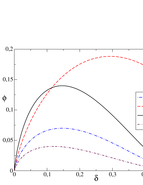
Figure 1: Bounds for $\varphi_{c}$. The VG lower bound is $\varphi_{c}\geq 0$. The upper bounds $\varphi_{max}(\delta)$ (26), dashed line, and $\varphi_{MRRW}(\delta)$ (32), full line, are reported. The lower bound to $D(\delta)$ obtained by Samorodnitsky, $\varphi_{S}(\delta)=\varphi_{MRRW}(\delta)/2$, is reported as a dot-dashed line. Finally, the value of $\varphi_{HNC}(\delta)$, below which our solution for the liquid state is well defined, is reported as a dot-dashed-dashed line.

In the literature the Delsarte method has been often formulated in terms of the function $A_{i}=\delta_{i0}+\rho\binom{n}{i}g(i)$, see e.g. BJ01 ; Sa01 . Conditions i)-ii) are equivalent to $A_{0}=1$, $A_{i}=0$ for $1\leq i<d$ and $A_{i}\geq 0$. Condition iii) gives, using Eq.s (16) and (17), and recalling that ${\cal F}_{n}(a,0)=1$, ${\cal F}_{n}(0,i)=\binom{n}{i}$ and $\sum_{i=0}^{n}{\cal F}_{n}(a,i)=2^{n}\delta_{a0}$ (being the Fourier transform of the function 1):

$$\begin{split}S(a)&=1+\rho\widehat{h}(a)=1+\sum_{i=0}^{n}{\cal F}_{n}(a,i)[\rho g(i)-\rho]=1+\sum_{i=0}^{n}\frac{{\cal F}_{n}(i,a)}{\binom{n}{a}}\binom{n}{i}\rho g(i)-\rho 2^{n}\delta_{a0}\\ &=\binom{n}{a}^{-1}\sum_{i=0}^{n}{\cal F}_{n}(i,a)\left[\rho\binom{n}{i}g(i)+\delta_{0i}\right]-\rho 2^{n}\delta_{a0}=\binom{n}{a}^{-1}\sum_{i=0}^{n}{\cal F}_{n}(i,a)A_{i}-\rho 2^{n}\delta_{a0}\ .\end{split}$$ (29)

Thus the condition $S(a)\geq 0$ is equivalent to $\sum_{i=0}^{n}{\cal F}_{n}(i,a)A_{i}\geq 0$ for $a\neq 0$, while for $a=0$ we simply have $\sum_{i=0}^{n}A_{i}=N$ from Eq. (27). Then the bound (28) can be reformulated as

$$A(n,d)\leq\max\left[\,\sum_{i=0}^{n}A_{i}\,\left|\,A_{i}\geq 0\,\,\,\forall i\,;A_{0}=1\,;A_{1}=\cdots=A_{d-1}=0\,;\sum_{i=0}^{n}{\cal F}_{n}(i,a)A_{i}\geq 0\,\,\,\forall a\right.\right]\equiv D(n,d)\ .$$ (30)

Upper bounds for $A(n,d)$ can be derived by studying the dual to the linear problem (30), see e.g. BJ01 . In this way one can prove that (MRRW bound MRRW77 ), for $n\rightarrow\infty$:

$$D(\delta)\equiv\limsup_{n\rightarrow\infty,n/d\rightarrow\delta}\frac{1}{n}\log_{2}D(n,d)\leq H\left(\frac{1}{2}-\sqrt{\delta(1-\delta)}\right)\equiv R_{MRRW}(\delta)\ ,$$ (31)

that means that $R(\delta)$ verifies the same bound and

$$\varphi\leq v\left(\frac{1}{2}-\sqrt{\delta(1-\delta)}\right)-\ln 2+v(\delta)\equiv\varphi_{MRRW}(\delta)\ .$$ (32)

This bound has been (little) improved only for $\delta<0.273$ MRRW77 ; BJ01 .

By constructing an explicit solution to the positivity conditions, one can obtain lower bounds on $D(\delta)$ (but this is not sufficient to have the same bound for $R(\delta)$, To06 ; Le06 ). For this problem, this has been done in Sa01 , where it was shown that

$$g(i)=(d+1)\delta_{id}+\theta(i-d)\ ,$$ (33)

where $\theta(i-d)=1$ for $i>d$ and $0$ otherwise, verifies conditions i)-iii) up to a density $\varphi_{S}(\delta)=\varphi_{MRRW}(\delta)/2$.

To resume, the situation is the following:

• the VG bound states that the maximum density $\varphi_{c}\geq 0$;

• the MRRW bounds coming from the dual to (30) prove that $\varphi_{c}<\varphi_{MRRW}(\delta)$, Eq. (32) (with a little improvement for $\delta<0.273$, see BJ01 );

• the Delsarte’s method cannot be used to prove that the VG bound is tight, i.e. that $\varphi_{c}\leq 0$, as the lower bound on $D(\delta)$ obtained in Sa01 implies that the best upper bound from Delsarte’s method cannot be smaller than $\varphi_{MRRW}(\delta)/2$;

• moreover, recent arithmetical results for $n=1000$ BJ01 seems to indicate that the actual value of $D(\delta)$ might be close to the MRRW ones, i.e. much larger then the lower bound of Sa01 . This means that the MRRW bounds are probably very close to the best one can obtain from the Delsarte’s method (30).

The bounds above for $\varphi_{c}$ (summarized in Fig. 1) leave a large gap - at least of the order of $\varphi_{MRRW}(\delta)/2$, but probably of the order of $\varphi_{MRRW}(\delta)$ - and there are not so many ideas on how to improve them BJ01 . Note that, as discussed in the introduction, for $\delta>1/2$ one can prove that $R(\delta)=0$, so the size of the code is not exponential.

III The liquid phase at high density

In this section we will discuss some insight on the problem that comes from the physical intuition on the possible behavior of the system (6). We are not able to present rigorous results but we hope that the discussion below will lead to new ideas on how to rigorously improve the bounds on $R(\delta)$.

It is convenient to outline our basic ideas before going into the details of the calculations. We try to find a solution to the HNC equations (12), (24) (or to other approximate equations for the liquid) for $\varphi>0$ ($\varphi$ is defined in Eq. (8)). We assume here that any resummation will be equivalent for $n\rightarrow\infty$ as long as it includes the ring diagrams FP99 . Such a solution should clearly verify at least the positivity conditions i)-iii). However there can be many different solutions to these conditions that may not correspond to the high-density liquid. In particular the solution proposed by Samorodnitsky, Eq. (33), is not suitable to describe a liquid state, as we do not expect to observe a large number of particles in contact (represented by a peak at $i=d$) in the liquid phase. Thus we will first look for a function $g(i)$ verifying i)-iii), not showing large peaks and departing continuously from the step function for $\varphi\geq 0$. We will show in the following that such a function exists up to $\varphi=\varphi_{HNC}(\delta)<\varphi_{S}(\delta)$, see Fig. 1, and is indeed given by the step function plus an exponentially small correction in $n$. We interpret this solution as describing the liquid phase and show numerically that the solution of the HNC equations converges to this solution for $n\rightarrow\infty$.

Using the solution above we can compute the entropy of the liquid. A crucial observation is that this entropy becomes negative for $\varphi\sim\log(n)/n$, i.e. very close to the VG bound. This means that the liquid phase must become unstable below this value of density, as the entropy of a discrete system must be positive. We then expect that the system (6) will undergo a phase transition at a density $\varphi\leq\log(n)/n$.

This behavior closely resembles the behavior of hard spheres in the continuum in the limit of large space dimension. For this problem, we recently showed PZ06 that at a value of density close to the radius of convergence of the virial expansion (i.e. to the VG value) the liquid phase becomes unstable towards a glass phase where replica symmetry is broken. In the glass phase the pressure rapidly increases and diverges at a maximum density (for the glass) which is found to be of the same order of the glass transition density.

By analogy with the problem in the continuum, we argue that also in this problem a glass transition exists at a density $\varphi_{K}\leq\log(n)/n$ and that the glass phase should exist up to a maximum density with the same scaling in $n$. This means that, if no other phases exist, one should have $\varphi_{c}\sim\log(n)/n$, i.e. the VG bound should be tight. Unfortunately we are still not able to repeat the calculation of the equation of state of the glass - that was done in PZ06 for the problem in the continuum - for this problem; but we believe that the computation is feasible and we leave it for future work.

Clearly other phases may exist at least for some special values of $n$, $d$. For instance, we have some numerical evidence, for even $d$, of a first-order phase transition toward a phase in which particles only occupy a subspace of the Hamming space. We will discuss this issue below.

In the following we will try to make these arguments more precise.

III.1 The Fourier transform for $n\rightarrow\infty$

We begin by studying the properties of the Fourier transform of the delta function $g(j)=\delta_{ij}$, that is simply ${\cal F}_{n}(a,i)$, for $n\rightarrow\infty$. We define $k=a/n$ and $x=i/n$. We want to compute the function $f(k,x)$ defined by

$$\Phi(k,x)={\cal F}_{n}(nk,nx)\sim{\rm Re}\,e^{nf(k,x)}\ ,\hskip 10.0ptn\rightarrow\infty\ .$$ (34)

Using the fact that the poles of the gamma function $\Gamma(z)$ are in $z=-k$ with residual $(-1)^{k}/k!$, we can rewrite Eq. (16) as

$${\cal F}_{n}(a,i)=\int_{C}dz\Gamma(z)\frac{\Gamma(a+1)\Gamma(n-a+1)}{\Gamma(a+z+1)\Gamma(i+z+1)\Gamma(n-a-i-z+1)}\ ,$$ (35)

where the contour $C$ embraces the negative part of the real $z$ axis, see Fig. 2. Using the Stirling formula $\Gamma(n)\sim n^{n}e^{-n}\sqrt{2\pi n}$, we get, changing the integration variable to $\zeta=z/n$, and neglecting power-law prefactors,

$${\cal F}_{n}(nk,nx)=\int_{C}d\zeta\,e^{n[\zeta\log\zeta-v(k)-(k+\zeta)\log(k+\zeta)-(x+\zeta)\log(x+\zeta)-(1-k-x-\zeta)\log(1-k-x-\zeta)]}=\int_{C}d\zeta\,e^{n\sigma(\zeta)}\ ,$$ (36)

and we can evaluate the integral using the saddle point method. The saddle point equation is

$$\frac{\zeta(1-k-x-\zeta)}{(k+\zeta)(x+\zeta)}=1\ ,$$ (37)

with solutions

$$\zeta_{\pm}=\frac{1}{2}\left[\frac{1}{2}-k-x\right]\pm\frac{1}{2}\sqrt{\left(k-\frac{1}{2}\right)^{2}+\left(x-\frac{1}{2}\right)^{2}-\frac{1}{4}}\ .$$ (38)

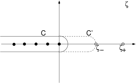
Figure 2: Left: the domain in the plane $(k,x)$ where the saddle points (38) are complex is represented by region A. Right: deformation of the integration contour to include the saddle point $\zeta_{-}$ (this plot refers to region B, see text).

From the analysis of the position of the solutions in the complex plane one can deduce the following:

1. In the region $\left(k-\frac{1}{2}\right)^{2}+\left(x-\frac{1}{2}\right)^{2}-\frac{1}{4}\leq 0$ (region A in Fig. 2) the solutions are complex, and $\zeta_{+}=\zeta_{-}^{*}$, $\sigma(\zeta_{+})=[\sigma(\zeta_{-})]^{*}$. Thus one has

   $${\cal F}_{n}(nk,nx)\sim e^{n\sigma(\zeta_{-})}+e^{n\sigma(\zeta_{+})}={\rm Re}\,e^{n\sigma(\zeta_{-})}\sim e^{n{\rm Re}\,\sigma(\zeta_{-})}\cos[n{\rm Im}\,\sigma(\zeta_{-})]\hskip 10.0pt\Rightarrow\hskip 10.0ptf(k,x)=\sigma(\zeta_{-})\ .$$ (39)

2. In region B of Fig. 2 the saddle points are real and positive with $0\leq\zeta_{-}\leq\zeta_{+}$, and $\sigma(\zeta_{\pm})$ are also real with $\sigma(\zeta_{+})>\sigma(\zeta_{-})>0$. The point $\zeta_{-}$ is then the closest saddle point to the original integration contour; moreover, it is a local mimimum of $\sigma(\zeta)$ along the real axis, so it is a maximum of $\sigma(\zeta)$ along the imaginary direction and the integration path can be deformed to include it without crossing regions of $\zeta$ where ${\rm Re}\,\sigma(\zeta)>\sigma(\zeta_{-})$, see Fig. 2. Then

   $${\cal F}_{n}(nk,nx)\sim e^{n\sigma(\zeta_{-})}\hskip 10.0pt\Rightarrow\hskip 10.0ptf(k,x)=\sigma(\zeta_{-})\ .$$ (40)

3. The behavior in the regions C,D,E can be obtained using the symmetries (18), (19), (20). Alternatively one can always choose the closest saddle point to the integration path that is a local minimum on the real axis: it turns out that one has to choose $\zeta_{-}$ in the region E and $\zeta_{+}$ in the regions C and D. With this choice the symmetries (18), (19), (20) are respected.

Finally one obtains

$$f(k,x)=\min_{{\rm Re}\,}[\sigma(\zeta_{+}),\sigma(\zeta_{-})]\ ,$$ (41)

where $\min_{\rm Re}\,$ means that one has to take the solution with the smallest real part. The real part of the resulting function $f(k,x)$ is an increasing function of $x$ for all $k$ and $x<1/2$, see Fig. 3. This allows to compute the Fourier transform of the theta function $\theta(d-i)$ for $d<n/2$. Defining $f_{x}(k,x)=\partial_{x}f(k,x)$, we have

$$\begin{split}\widehat{\theta}_{\delta}(nk)&=\sum_{i=0}^{n}{\cal F}_{n}(nk,i)\theta(d-i)\sim n{\rm Re}\,\int_{0}^{\delta}dx\,e^{nf(k,x)}\sim n{\rm Re}\,\int_{0}^{\delta}dx\,e^{n[f(k,\delta)+f_{x}(k,\delta)(x-\delta)+\cdots]}\\ &\sim{\rm Re}\,\frac{e^{nf(k,\delta)}}{f_{x}(k,\delta)}\sim\Phi(k,\delta)\ ,\end{split}$$ (42)

i.e. the Fourier transform of the theta coincides with the one of the delta to leading order in $n$ as long as $d<n/2$. Similarly we can compute the Fourier transform of a function that vanishes outside a finite interval and approaches zero linearly at the edge of the interval, i.e. $h(i)=\theta(d-i)(d-i)$:

$$\begin{split}\widehat{h}(nk)&\sim n^{2}{\rm Re}\,\int_{0}^{\delta}dx\,e^{nf(k,x)}(\delta-x)\sim n^{2}{\rm Re}\,\int_{0}^{\delta}dx\,e^{n[f(k,\delta)+f_{x}(k,\delta)(x-\delta)+\cdots]}(\delta-x)\\ &\sim{\rm Re}\,e^{nf(k,\delta)}\frac{1}{[f_{x}(k,\delta)]^{2}}\sim\Phi(k,\delta)\ ,\end{split}$$ (43)

i.e. to leading order in $n$ also this function is equal to $\Phi(k,\delta)$.

III.2 HNC for $n\rightarrow\infty$

Figure 3: The function ${\rm Re}\,f(k,x)$ for different values of $k$ as a function of $x$; from top to bottom $k=0.1,0.2,0.3,0.4,0.5$. Recall that from Eq. (18) ${\rm Re}\,f(k,x)={\rm Re}\,f(1-k,x)$.

We argue that for $n\rightarrow\infty$ the solution to the HNC equation approaches a solution of conditions i)-iii) which shows no large peaks. In particular we will look for a solution of the form $g(i)=\theta(i-d+1)[1+\exp(n\widetilde{h}(i))]$, $\widetilde{h}(i)\leq 0$, i.e. a solution differing from the step function (that describes the liquid for $\varphi<0$) by an exponentially small quantity. Conditions i)-iii) are, for $x=i/n$ and $k=a/n$, and recalling that $h(i)=g(i)-1$,

$$\begin{cases}\rho\widehat{h}(k)\geq-1\ ,\\ h(x)\geq-1\ ,\\ h(x)=-1\ ,\hskip 30.0ptx\leq\delta\ .\end{cases}$$ (44)

First we will check that for $\varphi<0$ the step function $g(x)=\theta(x-\delta)$, i.e. $h(x)=-\theta(\delta-x)$, satisfies the conditions above. Using Eq.s (10) and (42),

$$\rho\widehat{h}(k)=-\rho\Phi(k,\delta)\geq-1\hskip 10.0pt\Leftrightarrow\hskip 10.0pt{\rm Re}\,e^{n[\varphi-v(\delta)+f(k,\delta)]}=e^{n[\varphi-v(\delta)+{\rm Re}\,f(k,\delta)]}\cos[n{\rm Im}\,f(k,\delta)]\leq 1\ ,$$ (45)

and the latter relation is equivalent to

$${\rm Re}\,f(k,\delta)\leq v(\delta)-\varphi\ .$$ (46)

In Fig. 4 the function ${\rm Re}\,f(k,\delta)$ is reported as a function of $k$ for a representative value of $\delta$. It assumes its maximum in $k=0$ and $k=1$ and $f(0,\delta)=v(\delta)$. Thus the inequality (46) is always satisfied if $\varphi\leq 0$, so that in this region (which is also the region where the virial series converges) we argue that $h(x)=-\theta(\delta-x)$ describes the liquid phase for $n\rightarrow\infty$. This can also be checked by a direct evaluation of the leading terms in the (convergent) virial series, see FP99 . Following FP99 we also argue that the HNC resummation contains all the relevant diagrams for $\varphi<0$, so we can use it to obtain the free energy of the liquid. Substituting the result for $h(x)$ in Eq. (23) the last term is exponentially small in $n$ and one obtains, up to exponentially small corrections,

$$\begin{split}&\Psi(\rho)=-S(\rho)=\frac{\rho V_{d}}{2}+\ln\rho-1\ ,\\ &\widetilde{P}\equiv\frac{P}{\rho}=\rho\frac{d\Psi}{d\rho}=1+\frac{\widetilde{\rho}}{2}\ ,\end{split}$$ (47)

where $\widetilde{P}$ is the reduced pressure. As found in FP99 we find that the entropy is given by the ideal gas term plus the first virial correction. Note that $\widetilde{\rho}$ is exponentially small for $\varphi<0$ so the system behaves essentially as an ideal gas.

For $\varphi>0$ the function $h(x)$ cannot be given by $-\theta(\delta-x)$ as this function does not respect the positivity conditions (44). We follow the strategy of PS00 and decompose $h(x)=h_{0}(x)+h_{1}(x)$ assuming that $h_{0}(x)$ vanishes for $x>\delta$ and $h_{1}(x)$ is a continuous function of $x$. We call $Y\equiv h_{1}(\delta)=-1-h_{0}(\delta^{-})$, i.e. $h_{0}(\delta^{-})=-(1+Y)$. As $h_{0}(x)$ vanishes for $x>\delta$, its Fourier transform is given by (42):

$$\widehat{h}_{0}(k)=-(1+Y)\Phi(k,\delta)\ ,$$ (48)

and the condition $\rho\widehat{h}(k)=\rho\widehat{h}_{0}(k)+\rho\widehat{h}_{1}(k)\geq-1$ becomes

$$\widehat{h}_{1}(k)\geq-\frac{1}{\rho}+(1+Y)\Phi(k,\delta)\ .$$ (49)

We choose the simplest solution to the previous equation,

$$\widehat{h}_{1}(k)=\begin{cases}-\frac{1}{\rho}+(1+Y)\Phi(k,\delta)\hskip 30.0pt\text{for }-\frac{1}{\rho}+(1+Y)\Phi(k,\delta)\geq 0\ ,\\ 0\hskip 114.0pt\text{for }-\frac{1}{\rho}+(1+Y)\Phi(k,\delta)<0\ ,\end{cases}$$ (50)

and we will show that it gives, in real space, an exponentially small correction with respect to the step function. The function $\widehat{h}_{1}(k)$ has a two singularities when

$$(1+Y)\rho\Phi(k,\delta)=1\hskip 10.0pt\Leftrightarrow\hskip 10.0pt\varphi-v(\delta)+f(k,\delta)+\frac{1}{n}\ln(1+Y)=0\ ,$$ (51)

but the above equation is well defined only if its solutions lie in the region where $f(k,\delta)$ is real, otherwise the function $\Phi(k,\delta)$ will oscillate very fast. This will impose some restrictions to the values of $\varphi$ and $d$.

Figure 4: The function ${\rm Re}\,f(k,\delta)$ as a function of $k$ for $\delta=0.1$. The value of $v(\delta)$ and of $v(\delta)-0.05$ are also reported. The value of $k$ such that ${\rm Re}\,f(k,\delta)$ intersects $v(\delta)-\varphi$ is the value of $k_{c}(\delta,\varphi)$, see Eq. (53).

First we will restrict to odd $d$ in order to have the symmetry $\Phi(1-k,\delta)=\Phi(k,\delta)$; for even $d$ we have the opposite symmetry $\Phi(1-k,\delta)=-\Phi(k,\delta)$ and $f(k,\delta)$ has an imaginary part for $k>1/2$. This follows from $\Phi(k,\delta)={\cal F}_{n}(a,d)$ (with $a=nk$ and $d=n\delta$) and from Eq. (18). For odd $d$ Eq. (51) will have two solutions $k_{c}$, $1-k_{c}$ due to the symmetry, see Fig. 4. Note that the opposite restriction was applied in the numerical computation of BJ01 where only the case of even $d$ has been considered.

Next, we look for a solution $k_{c}$ outside the region A of Fig. 2, as in region A we already know that $f(k,\delta)$ is not real. This means that the maximum possible value for $k_{c}$ is

$$k_{max}(\delta)=\frac{1}{2}-\sqrt{\frac{1}{4}-\left(\delta-\frac{1}{2}\right)^{2}}=\frac{1}{2}-\sqrt{\delta(1-\delta)}\ ,$$ (52)

that is the boundary of the region where $f(k,\delta)$ is real, see Fig. 2.

As we will self-consistently verify at the end, under the restrictions above one has $Y\sim e^{-n\kappa}$, then Eq. (51) becomes

$$f(k,\delta)=v(\delta)-\varphi\ .$$ (53)

For $\varphi\leq 0$ it has no solutions as discussed above, so $\widehat{h}_{1}(k)=0$, then $h_{1}(x)=0$, $Y=0$ and we recover the step function solution. For $\varphi>0$, $k_{c}$ increases from $0$ to $k_{max}(\delta)$ and reaches the boundary of region A, using Eq. (53), exactly at

$$\varphi=v(\delta)-f(k_{max}(\delta),\delta)=\varphi_{MRRW}(\delta)/2=\varphi_{S}(\delta)\ ,$$ (54)

where $\varphi_{MRRW}(\delta)$ has been defined in Eq. (32).

We have now to compute $h_{1}(x)$ from $\widehat{h}_{1}(k)$. The function $\widehat{h}_{1}(k)$ verifies $\widehat{h}_{1}(k)=\widehat{h}_{1}(1-k)$ and is nonzero only for $k<k_{c}$ and $k>1-k_{c}$; it vanishes linearly close to $k_{c}$, $\widehat{h}_{1}(k)\sim(1+Y)\Phi_{k}(k_{c},\delta)(k-k_{c})$, and $\Phi_{k}(k,\delta)=\partial_{k}\Phi(k,\delta)$ is real in $k=k_{c}$. If we restrict to even $i$, we have also $\Phi(x,k)=\Phi(x,1-k)$ by symmetry (19). We can do that because it is possible to show that, in the case of odd $d$ that we are considering, one has $h(i-1)=h(i)$ for even $i$; thus it is enough to compute $h(i)$ for even $i$ (see the next section, Appendix A and Fig. 6 for a detailed discussion of this tricky point). Using Eq. (43) we have then

$$\begin{split}h_{1}(x)&=\frac{2n}{2^{n}}\int_{0}^{1/2}dk\,\Phi(x,k)\widehat{h}_{1}(k)\sim\frac{2n}{2^{n}}(1+Y)e^{nf(k_{c},\delta)}nf_{k}(k_{c},\delta)\,{\rm Re}\,\int_{0}^{k_{c}}dk\,e^{nf(x,k)}(k-k_{c})\\ &\sim\frac{1+Y}{2^{n-1}}e^{nf(k_{c},\delta)}\,{\rm Re}\,e^{nf(x,k_{c})}\frac{f_{k}(k_{c},\delta)}{[f_{x}(x,k_{c})]^{2}}\ .\end{split}$$ (55)

Keeping only the leading terms (exponentials of $n$) we obtain the self consistency equation for $Y$:

$$Y=h_{1}(\delta)=(1+Y)e^{n[f(k_{c},\delta)+f(\delta,k_{c})-\ln 2]}\ .$$ (56)

If $k_{c}<k_{max}$ we have $f(k_{c},\delta)+f(\delta,k_{c})-\ln 2<0$, so that $Y$ is exponentially small and is given by

$$Y=e^{n[f(k_{c},\delta)+f(\delta,k_{c})-\ln 2]}=e^{n[v(\delta)+v(k_{c})-2\varphi-\ln 2]}\ .$$ (57)

where we used the relation $f(x,k)=f(k,x)+v(k)-v(x)$ that follows from Eq. (17) and Eq. (53). Finally, the function $\widehat{h}(k)=\widehat{h}_{0}(k)+\widehat{h}_{1}(k)$ is given, using Eq. (50) and $Y\ll 1$, by

$$\rho\widehat{h}(k)=\begin{cases}-1\hskip 80.0pt\text{for }k<k_{c}\text{ and }k>1-k_{c}\ ,\\ -\rho\Phi(k,\delta)\hskip 50.0pt\text{for }k_{c}<k<1-k_{c}\ .\end{cases}$$ (58)

We can rewrite Eq. (55) using $Y\ll 1$, neglecting non-exponential prefactors, and recalling that $f(k_{c},\delta)=v(\delta)-\varphi$, as

$$h_{1}(x)=\frac{e^{n[v(\delta)-\varphi]}}{2^{n}}\Phi(x,k_{c})=\frac{1}{\rho}\frac{1}{2^{n}}\Phi(x,k_{c})\ ;$$ (59)

note that from Eq. (16) it follows that $2^{-n}\Phi(x,k_{c})$ is the Fourier transform of $\delta(k-k_{c})$. Finally, $h(x)$ is given, from Eq. (55), by

$$\begin{split}&h(x)=\begin{cases}-1\hskip 35.0ptx<\delta\ ,\\ {\rm Re}\,e^{n\widetilde{h}(x)}\hskip 22.0ptx\geq\delta\ ,\end{cases}\\ &\widetilde{h}(x)=v(\delta)-\varphi+f(x,k_{c})-\ln 2\ .\end{split}$$ (60)

The solution above is defined up to the value $\varphi_{S}$ of the density given by Eq. (54). Indeed, the solution $k_{c}$ of Eq. (51) is given by Eq. (53) only if it is in the region where $f(k,\delta)$ is real. Otherwise, oscillations are present in $\Phi(k,x)$ and the solution is not well defined. Moreover, if $Y$ is not exponentially small again the solution above fails. Both these conditions seem to be violated for $\varphi>\varphi_{S}(\delta)$.

There is however another condition to be imposed, namely that $\widetilde{h}(x)\leq 0$; otherwise the solution will be exponentially large and again we do not expect that for a liquid phase. The maximum of $\widetilde{h}(x)$ is attained in $x=0$, $x=1$, and is given by $v(\delta)+v(k_{c})-\varphi-\ln 2$. The condition $\widetilde{h}(x)\leq 0$ then requires

$$v(\delta)+v(k_{c})-\varphi-\ln 2\leq 0\ .$$ (61)

A numerical solution of the previous equation (recall that $k_{c}$ depends implicitly on $\varphi$) gives the stability threshold $\varphi_{HNC}(\delta)$, which is reported in Fig. 1. For $\varphi\geq\varphi_{HNC}$ our solution starts to exhibit diverging oscillations at large $x$. This is observed also in the numerical solution of the HNC equations, see below. Above $\varphi_{S}(\delta)$ either the solution does not exist anymore or it yields a value of $Y$ that is exponentially diverging with $n$. In both cases the solution does not describe a liquid phase. We will see however that we are not really interested in so high values of the density as the liquid phase becomes unstable at a much lower density.

III.3 HNC entropy

The HNC free energy is the canonical free energy, that for hard spheres is simply $-S(\rho)$. For $\varphi\leq 0$ it is given by Eq. (47), and we showed that for $\varphi>0$ only exponentially small corrections appear. Neglecting these corrections we have from Eq. (47)

$$S(\rho)=1-\log\rho-\frac{1}{2}\rho V_{d}\sim 1-n\varphi+nv(\delta)-\frac{1}{2}\log[2\pi\delta(1-\delta)]-\frac{1}{2}\log n-\frac{1}{2}e^{n\varphi}\ ,$$ (62)

in the full range $\varphi<\varphi_{HNC}(\delta)$. An interesting observation is that $S(\rho)$ becomes negative at a value of density given by, keeping only the leading terms,

$$S(\varphi)\sim-n\varphi+nv(\delta)-\frac{1}{2}\log n-\frac{1}{2}e^{n\varphi}=0\ ,$$ (63)

and the solution is, at first order in $n\rightarrow\infty$,

$$\varphi_{0}=\frac{1}{n}\log[2nv(\delta)-3\log n]\ .$$ (64)

As for a discrete system $S(\varphi)\geq 0$, this means that the liquid phase must become unstable at a density $\varphi<\varphi_{0}\sim\log(n)/n$.

III.4 Numerical solution of the HNC equations

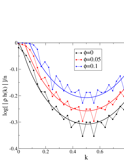
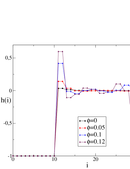
Figure 5: Comparison of the numerical solution of the HNC equations with the asymptotic solution of the positivity conditions. Left: The function $\ln[|\rho\widehat{h}(k)|]/n$ obtained numerically is reported as a function of $k$ for $n=36$ and $d=11$ (i.e. $\delta=0.305$) and $\varphi=0,0.05,0.1$. The lines are obtained from Eq. (65). Right: The function $h(i)$ for $n=36$, $d=11$ and $\varphi=0,0.05,0.1,0.12$. At large $\varphi$ we start to observe diverging oscillations at high values of $i$, see text.

We will now compare the asymptotic solution with a numerical solution of the HNC equations (24). The latter are solved using a standard iterative algorithm. For graphical convenience we report the function $\frac{1}{n}\log|\rho\widehat{h}(k)|$, that from Eq. (58) is given by

$$\lim_{n\rightarrow\infty}\frac{1}{n}\log|\rho\widehat{h}(k)|=\begin{cases}0\hskip 220.0pt\text{for }k<k_{c}\text{ and }k>1-k_{c}\ ,\\ {\rm Re}\,f(k,\delta)+\varphi-v(\delta)+\frac{1}{n}\log|\cos n{\rm Im}\,f(k,\delta)|\hskip 30.0pt\text{for }k_{c}<k<1-k_{c}\ .\end{cases}$$ (65)

The last term is nonzero only for $k\in[k_{max}(\delta),1-k_{max}(\delta)]$ and gives rise to oscillations whose frequency increases on increasing $n$. Moreover at the values of $k$ where $\cos n{\rm Im}\,f(k,\delta)=0$ the last term diverges. These values accumulate in the interval $k\in[k_{max}(\delta),1-k_{max}(\delta)]$ for large $n$. However, for the relativaly small values of $n$ considered here, the are no integer values of $a=nk$ where $\cos n{\rm Im}\,f(k,\delta)=0$ and we can compare the function $\frac{1}{n}\log|\rho\widehat{h}(k)|$ with its asymptotic limit neglecting the last term. Moreover we can compare $h(i)$ with the analytical expression (60). The comparisons are encouraging as shown in Fig. 5. We find that $\widehat{h}(k)$ agrees well with Eq. (58) and, for small $\varphi$, $h(i)$ is essentially the step function plus a small corrrection. On increasing the density large oscillations appear at large $i$, as predicted by Eq. (60). Unfortunately a quantitative comparison of $h(i)$ with the asymptotic expression requires either the evaluation of finite $n$ corrections, due to the small values of $n$ we can investigate numerically, or the (difficult) investigation of much larger values of $n$, see e.g. BJ01 .

III.5 Is there a glass transition?

The fact that the entropy becomes negative seems to indicate the existence of a phase transition. By analogy with the continuum problem, where we showed that a glass transition happens at a similar value of the density PZ06 , we can conjecture that a glass transition will happen also in this problem.

If this is the case, one can show by general arguments and by analogy with the continuum problem that $S_{glass}(\varphi)\leq S_{liquid}(\varphi)$ (this is because a downward jump of the compressibility is expected at the glass transition PZ05 ). This means that the entropy of the glass will vanish at a density $\varphi<\varphi_{0}\sim\log(n)/n$. Then both the liquid and the glass phase will disappear for $\varphi\sim\log(n)/n$. If there are no other phases (such as a “crystal”), this scenario indicates that the Varshamov-Gilbert bound should give asymptotically the exact result.

Note also that the correlation function used by Samorodnitsky, Eq. (33) is similar to the one we expect for the glass phase (see the discussion in PZ05 ; PZ06 ). This means that, if the picture above is correct, the $g(i)$ in Eq. (33) should correspond to realizable packings only up to a density $\varphi\sim\log(n)/n$. We hope that further work will clarify this issue, see also the discussion in To06 ; Le06 .

III.6 Other instabilities

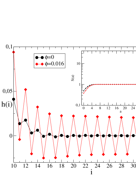
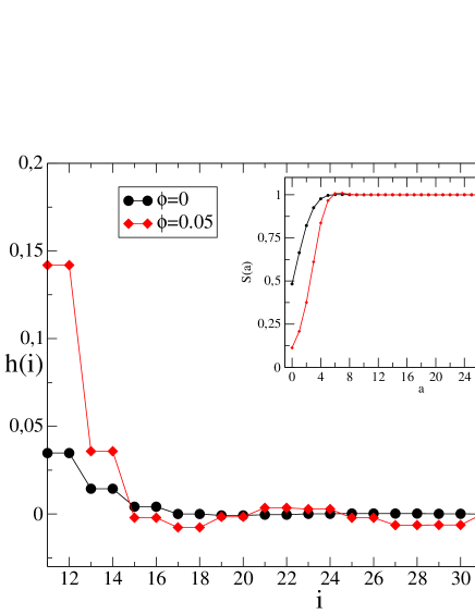
Figure 6: Left: correlation function $h(i)$ for $n=36$, $d=10$ and $\varphi=0,0.016$. Inset: structure factor $S(a)=1+\rho\widehat{h}(a)$ for the same values of the parameteres. On increasing $\varphi$ above $\varphi=0$ strong oscillations appear in $h(i)$, related to a strong peak in $S(a)$ for $a=36$. Right: same plot for $n=36$, $d=11$ and $\varphi=0,0.05$. In this case the oscillations are absent, $S(a)$ has a different behavior for large $a$, and $h(i)$ decays in steps of two. The different (approximate) symmetry of $S(a)$ is related to the symmetry (18).

We would like now to consider a different instability of the liquid that is observed for even $d$. Indeed, $d$ is the smallest possible distance between any pair of spheres. Let us split the Hamming space $H^{n}_{2}$ into two spaces $H^{n}_{2}=H^{n}_{e}\cup H^{n}_{o}$, where $H^{n}_{e}\equiv\{s\in H^{n}_{2}|d(s,0)\text{ is even}\}$ and $H^{n}_{o}\equiv\{s\in H^{n}_{2}|d(s,0)\text{ is odd}\}$. Recall that $\rho g(i)=\rho[1+h(i)]$ is the probability of finding a particle in a given point at distance $i$ from the origin, given that there is a particle in the origin.

At high density, given that there is a sphere $s_{0}$ in the origin, it will be convenient, say, to place the second sphere $s_{1}$ at the minimum distance $d$, thus $s_{1}\in H^{n}_{e}$. Then we can put another sphere $s_{2}$ at minimum distance $d$ from $s_{1}$, so that $s_{2}\in H^{n}_{e}$, and so on. It is clear that this picture is oversimplified but still we can expect that at large enough density particles will concentrate on one of the subsets $H^{n}_{e,o}$, depending whether there is or not a particle in the origin.

This is indeed what we found in the solution of the HNC equations. The partial localization of the particles on a subset $H^{n}_{e,o}$ is revealed by oscillations in $h(i)$, which is much bigger on the even values of $i$, see Fig. 6. The oscillations in $h(i)$ are related to a strong peak developping in $S(a)=1+\rho\widehat{h}(a)$ for $a=n$ on increasing $\varphi$ above $0$. Due to this growing peak, the HNC equations rapidly become unstable for small values of $\varphi$ (much smaller than for odd $d$). Preliminary Montecarlo simulations seems to indicate the existence of a first order phase transition to a phase in which particles are completely localized on a sublattice at a critical value of $\varphi$.

For odd $d$ a related phenomenon occurs. Indeed, by looking at the correlation function $h(i)$ for odd $d$ (see right panel in Fig. 6), we see that we have $h(i)=h(i+1)$ for odd $i$, i.e. that the correlation function decays in steps of two. This can be understood by the following argument. Consider a system of sequences $s^{\prime}\equiv(s,s_{n+1})\in H^{n+1}_{e}$, i.e. with the constraint that $d^{\prime}(s^{\prime},0)$ is even, where $d^{\prime}(s^{\prime},0)=d(s,0)+s_{n+1}$ is the distance in the Hamming space $H^{n+1}_{2}$. This constraint fixes the last bit $s_{n+1}$: as $s_{n+1}=0$ if $d(s,0)$ is even and $s_{n+1}=1$ if $d(s,0)$ is odd. If we consider in the original space $H^{n}_{2}$ a sphere at distance $d(s,0)=i$ with $i$ odd we have $d^{\prime}(s^{\prime},0)=i+1$, but also if $d(s,0)=i+1$ we have $d^{\prime}(s^{\prime},0)=i+1$. Thus, spheres at distance $i$ and $i+1$ with $i$ odd have the same distance $i+1$ (even) from the origin in $H^{n+1}_{2}$.

This means that the original problem on $H^{n}_{2}$ with minimum distance $d$ odd can be mapped into a problem on $H^{n+1}_{e}$ with $d^{\prime}=d+1$ even. However, in the new problem, particles that were at a distance $i$ and $i+1$ from the (old) origin (for odd $i$) are at the same distance from the (new) origin, thus the probability to have a particle at distance $i$ (odd) and $i+1$ in the original problem, given that there is a particle in the origin, should be the same.

Note that the argument cannot be repeated for even $d$ as in this case we should map the problem into a problem on $H^{n+1}_{e}$ with distance $d^{\prime}$ odd, and this is inconsistent as discussed above.

IV Conclusions

We discussed the high-density behavior of a system of hard spheres on the hypercube $H^{n}_{2}$ from a physical point of view, trying to understand the mechanisms that determine the maximum density of the system.

First we found a possible asymptotic solution for the liquid correlation in the limit $n\rightarrow\infty$, and we showed that this solution yields a negative entropy for $\varphi\sim\log(n)/n$, i.e. for a number of particles $N\sim\frac{2^{n}}{V_{d}}n^{1/n}$, very close to the Varshamov-Gilbert lower bound.

On this ground we argue that a phase transition must exist towards a different phase. The nature of this transition is still unknown, but we presented some arguments in favor of a glass transition (basically, the analogy with the problem of hard spheres in $\hbox{\msytw R}^{n}$ for $n\rightarrow\infty$ PZ06 ) and for a first order transition toward a phase in which the particles are constrained to a sublattice $H^{n}_{o,e}$ for even $d$ (some insight from the solutions of the HNC equations and from preliminary Montecarlo simulations).

Both these possibilities require further investigation. In particular, the study of the glass transition requires the computation of the replicated partition function of the system following PZ05 ; PZ06 . This is more difficult in this discrete problem as we cannot make a Gaussian ansatz for the single particle density. The study of the first order transition will require more extensive numerical simulations.

Moreover, there is also the possibility that, at least for some particular values of $n$ and $d$, some particular “crystal-like” configurations of high density exist. Unfortunately, our approach is based on a low density expansion (the virial series) so it is unable to capture the existence of such special configurations.

The results presented here are not conclusive but in our opinion may lead to new ideas on how to improve the current bounds on $R(\delta)$. We hope, in particular, that future work will clarify whether a glass transition exist or not in this system.

Appendix A More on symmetries

We will discuss here the reason why we must restrict to even values of $i$ in computing $h_{1}(x)$, see Eq. (55). As we discussed in section III.6 for odd $d$ the function $h(i)$ has the property that $h(i-1)=h(i)$ for even $i$. This is a consequence of a hidden symmetry, namely the possibility to map the problem in $H^{n}_{2}$ in a problem in $H^{n+1}_{e}$.

It can be shown that if $h(i)$ has such a symmetry, its Fourier transform $\widehat{h}(a)$ has the symmetry $\widehat{h}(a)=\widehat{h}(n-a+1)$, $a=1,\cdots,n$, due to the structure of the matrix ${\cal F}_{n}(a,i)$. This is consistent with the observation that in the limit $n\rightarrow\infty$ with $a=nk$, $\widehat{h}(k)=\widehat{h}(1-k)$, as comes out from Eq. (58). However we are discarding a factor $1/n$.

When inverting the Fourier transform to recover $h(i)$, we find that if $i$ is even we get a meaningful result, while if $i$ is odd, the symmetry $\widehat{h}(k)=\widehat{h}(1-k)$, if interpreted as $\widehat{h}(a)=\widehat{h}(n-a)$ leads simply to $h(i)=0$ due to the symmetry (18). The direct computation of $h(i)$ for odd $i$ would require a more refined calculation, however it is much simpler to compute $h(i)$ for even $i$ and use the identity $h(i-1)=h(i)$.

This procedure seems to produce meaningful results as evidenced by the positive agreement with numerical data, see Fig. 5.

References

- (1) E. N. Gilbert, A comparison of signalling alphabets, Bell Syst. Tech. Jnl. 31, 504–522 (1952); R. R. Varshamov, Estimate of the number of signals in error correcting codes, Dokl. Akad. Nauk SSSR 117, 739–741 (1957).
- (2) P. Delsarte, An algebraic approach to the association schemes of coding theory, Philips Res. Rep. Suppl. 10, 1–97 (1973).
- (3) R. J. McEliece, E. R. Rodemich, H. Rumsey and L. R. Welch, New upper bounds on the rate of a code via the Delsarte-MacWilliams inequalities, IEEE Trans.Inform.Theory 23, 157–166 (1977).
- (4) A. Procacci and B. Scoppola, Statistical mechanics approach to coding theory, J. Stat. Phys. 96, 907–912 (1999).
- (5) A. Barg and D. B. Jaffe, Numerical results on the asymptotic rate of binary codes, in “Codes and Association Schemes” (A. Barg and S. Litsyn, Eds.), Amer. Math. Soc., Providence, 2001
- (6) A. Samorodnitsky, On the Optimum of Delsarte’s Linear Program, Journal of Combinatorial Theory, Series A 96, 261–287 (2001).
- (7) H. L. Frisch and J. K. Percus, High dimensionality as an organizing device for classical fluids, Phys. Rev. E 60, 2942–2948 (1999).
- (8) G. Parisi and F. Slanina, A toy model for the mean-field theory of hard-sphere liquids, Phys. Rev. E 62, 6554–6559 (2000).
- (9) G. Parisi and F. Zamponi, Amorphous packings of hard spheres in large space dimension, cond-mat/0601573.
- (10) O. U. Uche, F. H. Stillinger and S. Torquato, On the realizability of pair correlation functions, Physica A 360, 21–36 (2006); S. Torquato and F. H. Stillinger, New provisional lower bounds on the optimal density of sphere packings, submitted.
- (11) J.-P. Hansen and I. R. MacDonald, Theory of simple liquids (Academic Press, London, 1986).
- (12) Eric W. Weisstein, Krawtchouk Polynomial, From MathWorld–A Wolfram Web Resource, http://mathworld.wolfram.com/KrawtchoukPolynomial.html
- (13) A. Lenard, States of classical statistical mechanics of infinitely many particles: I, II, Arch. Rational. Mech. Anal. 59, 219–239, 241–256 (1975).
- (14) T. Kuna, J. L. Lebowitz and E. Speer, On the realizability of point processes with specified one and two particle densities, in Math.Frosch.Oberwolfach 43 (2004), Large Scale Stochastic Dynamics, ed. C. Landim, S. Olla, and H. Spohn; O. Costin and J. L. Lebowitz, On the construction of particle distributions with specified single and pair densities, J. Phys. Chem. 108, 19614 (2004).
- (15) G. Parisi and F. Zamponi, The ideal glass transition of hard spheres, J. Chem. Phys. 123, 144501 (2005).