Breakdown of Luttinger’s theorem in two-orbital Mott insulators

Abstract

An analysis of Luttinger’s theorem shows that – contrary to recent claims – it is not valid for a generic Mott insulator. For a two-orbital Hubbard model with two electrons per site the crossover from a non-magnetic correlated insulating phase (Mott or Kondo insulator) to a band insulator is investigated. Mott insulating phases are characterized by poles of the self-energy and corresponding zeros in the Greens functions defining a “Luttinger surface” which is absent for band insulators. Nevertheless, the ground states of such insulators with two electrons per unit cell are adiabatically connected.

The basic quantity which defines a metal at low temperatures is the Fermi surface. Excitations of the Fermi surface are the basis of Fermi liquid theory. The concept of the Fermi surface also allows to distinguish different phases. Changes in the topology of the Fermi surfaces (e.g. vanishing bands) are therefore always associated with quantum phase transitions.

Does an analog quantity exist in the case of a Mott insulator where strong interactions prohibit the formation of a Fermi surface? In a number of recent papers dzyaloshinskii ; tsvelik1 ; tsvelik2 ; yang ; stanescu ; berthod it has been argued that in such a situation the concept of a Fermi surface has to be replaced by the so-called “Luttinger surface”. While the Fermi surface is defined by poles of the Greens function, the Luttinger surface is obtained from the zeros of the Greens function or, equivalently, from the poles of the self-energy.

This identification is motivated by Luttinger’s theorem luttinger , which states that at zero temperature, $T=0$, the total density of electrons $n$ can be obtained by summing up all momenta where the real part of the Greens function evaluated at the Fermi energy is positive. For a multiband system the propagator is a matrix. Denoting the eigenvalues of this matrix by $G_{\alpha}(\omega,{\mathbf{p}})$ and using that $\text{Im}\,G_{\alpha}(0,{\mathbf{p}})=0$, Luttinger’s theorem (also called Luttinger’s sum rule) takes the form

$$n=2\sum_{\alpha}\int_{G_{\alpha}(\omega=0,{\mathbf{p}})>0}\frac{d^{3}{\mathbf{p}}}{(2\pi)^{3}}$$ (1)

It claims that the total density of electrons is fixed by the volume enclosed by a surface where the zero-frequency propagator $G(0,{\mathbf{p}})$ changes sign (alternative versions of the theorem are briefly discussed in Sec. 4). As emphasized recently by Dzyaloshinskii dzyaloshinskii and by Essler and Tsvelik tsvelik1 , there are two ways how such a sign change can happen. At a Fermi surface, $E({\mathbf{p}})=\mu$, there is a pole, $G(\omega,{\mathbf{p}})\approx\frac{Z_{\mathbf{p}}}{\omega-(E({\mathbf{p}})-\mu)}$, where $Z_{\mathbf{p}}$ and $E_{\mathbf{p}}$ are the weight and dispersion of the quasi particle. Alternatively, the propagator can change its sign going through zero instead of infinity, $G(\omega=0,{\mathbf{p}})=0$. The latter condition defines the “Luttinger surface” which is realized in Mott insulators dzyaloshinskii ; tsvelik1 ; tsvelik2 . This concept was for example used by Yang, Rice and Zhang yang to build up a phenomenological theory of the pseudogap state. In a recent preprint, Stanescu, Phillips and Choy stanescu tried to explore the role of Luttinger surfaces for (doped) Mott insulators. Recently, Ortloff, Balzer and Potthoff potthoff07 investigated under what conditions various (non-perturbative) approximation schemes lead to a violation of the Luttinger theorem.

This motivates us to investigate the question whether the concept of such a Luttinger surface is as general and robust as the Fermi surface. Can one conclude that two states with a different topology of Luttinger surfaces have to be separated by a quantum phase transition? In Ref. tsvelik2 , Konik, Rice and Tsvelik have for example constructed a doped spin liquid (by coupling Mott-insulating Hubbard ladders) which is characterized both by a Luttinger surface and by the Fermi surfaces of small particle and hole pockets. Here the question arises whether this seemingly exotic state of matter is adiabatically connected to a weakly interacting system where Luttinger surfaces are absent.

In the following we will first show that Luttinger’s theorem (1) is not valid for a generic Mott insulator using an explicit counter example. We will then discuss which assumptions underlying its proof may not be fulfilled and finally investigate implications for the question whether various insulating states are adiabatically connected.

1 Model

For definiteness, the following two-band Hubbard model is considered

$$H = H_{kin}+\sum_{i}H^{i}_{\text{loc}}$$ (2)

$$H_{kin} = \sum_{ij\alpha}t_{ij}^{\alpha}c^{\dagger}_{\alpha i\sigma}c_{\alpha j\sigma}$$ (3)

$$H^{i}_{\text{loc}} = V(c^{\dagger}_{1i\sigma}c_{2i\sigma}+c^{\dagger}_{2i\sigma}c^{\ }_{1i\sigma})+J{\mathbf{S}}_{1i}{\mathbf{S}}_{2i}$$ (4)

$$+\sum_{\alpha=1}^{2}\left[(\epsilon_{\alpha}-\mu)c^{\dagger}_{\alpha i\sigma}c_{\alpha i\sigma}+U_{\alpha}n_{\alpha i\uparrow}n_{\alpha i\downarrow}\right]$$

where $\alpha=1,2$ is the orbital index, ${\mathbf{S}}_{\alpha i}$ the spin at site $i$ in band $\alpha$ and $n_{\alpha i\sigma}$ the number of spin $\sigma$ electrons at site $i$ in band $\alpha$. The model (2) and various limits of it (which include the Anderson lattice or Kondo lattice, models for bilayer compounds or multi-orbital systems) have been widely studied.

The main motivation why we are interested in the model (2) in the context of this paper (rather than e.g. the one-band Hubbard model) is that it has a simple, almost trivial limit which allows us to discuss the validity of Luttinger’s theorem for Mott insulators and crossovers between different types of insulators. We consider the limit where (i) the system is half-filled as there are two electrons per unit cell, (ii) the ground-state of $H_{\text{loc}}^{i}$ is a singlet separated by a gap $\Delta$ from all excited states (see Appendix A), and (iii) the hopping is very small, $t\ll\Delta$. The physics of this limit can be fully understood using a straightforward strong coupling expansion around the atomic limit, $H_{kin}=0$ (performed e.g. up to 11th order in Ref. monien for a Kondo insulator). In contrast, the Mott insulating phase of the single-band Hubbard models is more difficult to analyze as the ground-state of $H_{\text{loc}}$ is spin-degenerate which usually leads to some form of magnetism (and also the zero-temperature non-magnetic state obtained e.g. within dynamical mean field theory is non-generic and responds in a singular way to tiny magnetic fields potthoff07 ). Within our model one can easily study the crossover from $\epsilon_{1}=\epsilon_{2}$, $V=0$ and $U_{\alpha}\gg t^{\alpha}$ where one has two coupled Mott insulators with $\Delta=3J/4$ and charge gap $U/2+3J/4$ to a band insulator with $U_{\alpha}=0$ and a large band gap $\Delta=\sqrt{\left(\frac{\epsilon_{1}-\epsilon_{2}}{2}\right)^{2}+V^{2}}$. Taking a slightly different limiting procedure [$U_{2}=2(\mu-\epsilon_{2})\to\infty,t^{2}_{ij}=0,U_{1}=0,V=0$ and $J>0$], the model (2) also describes a Kondo insulator, i.e. the insulating phase of a half-filled Kondo-lattice model.

2 Breakdown of Luttinger’s theorem

2.1 Local limit

First, two coupled Mott insulators are analyzed with $V=0,U_{1}=U_{2}=U,\epsilon_{1}=\epsilon_{2}=-U/2,t^{1}_{ij}=t^{2}_{ij}=t_{ij}$, $J,U\gg t_{ij}$ and $\mu$ chosen such that the system is half filled, $n=2$. For $t_{ij}=0$, the energy (per site) of the singlet ground-state is $-2\mu-3J/4$. The $T=0$ Greens function of each of the two bands is given by

$$G_{\text{loc}}(\omega)=\frac{1}{2}\left(\frac{1}{\omega+\mu-\tilde{U}/2}+\frac{1}{\omega+\mu+\tilde{U}/2}\right)$$ (5)

with $\tilde{U}=U+3J/2$. The corresponding local self-energy is given by

$$\Sigma_{\text{loc}}(\omega)=\frac{\tilde{U}}{2}+\frac{(\tilde{U}/2)^{2}}{\omega+\mu}.$$ (6)

This form of the self-energy is well known from the Hubbard I approximation hubbard1 which, indeed, correctly describes the zeroth order strong-coupling expansion (note, however, that we are not using the Hubbard I approximation in the following but instead a controlled strong-coupling expansion). To leading order in $t_{ij}$, the self-energy stays local and the Greens function is obtained as

$$G(\omega,{\mathbf{p}})=\frac{1}{\omega-[\epsilon_{\alpha}+t_{{\mathbf{p}}}-\mu+\Sigma_{\text{loc}}(\omega)]}$$ (7)

where the single-particle dispersion $t_{{\mathbf{p}}}$ is the Fourier transform of $t_{ij}$. To this order, the spectral function at momentum ${\mathbf{p}}$ consists of two delta-peaks approximately located at $\pm\frac{\tilde{U}}{2}+\frac{t_{\mathbf{p}}}{2}-\mu$ with weight $\frac{1}{2}\pm\frac{t_{\mathbf{p}}}{2\tilde{U}}$.

It is easy to see that Luttinger’s theorem is not valid for the Mott insulator discussed above. When the chemical potential is changed within the gap, $E_{-}<\mu<E_{+}$, the total density of electrons, $n=2$, on the left-hand side of Eq. (1) remains constant at $T=0$. Therefore the choice of the chemical potential is completely arbitrary in a grand-canonical ensemble at $T=0$, (see Sec. 2.3 for a discussion of a canonical ensemble with fixed particle number). At the same time, the right-hand side of Luttinger’s sum rule, Eq. (1), changes from $4$ to $0$ and is not constant, see Fig. 1. Using for example the leading order strong-coupling expansion, Eq. (7), one gets $G(\omega=0,{\mathbf{p}})>0$ for all momenta if $E_{-}<\mu<0$ and $G(\omega=0,{\mathbf{p}})<0$ for $0<\mu<E_{+}$ where

$$E_{-} \approx -\frac{\tilde{U}}{2}+\frac{\max_{\mathbf{k}}[t_{\mathbf{k}}]}{2}+O\!\left(\frac{t^{2}}{J},\frac{t^{2}}{U}\right)$$

$$E_{-} \approx \frac{\tilde{U}}{2}+\frac{\min_{\mathbf{k}}[t_{\mathbf{k}}]}{2}+O\!\left(\frac{t^{2}}{J},\frac{t^{2}}{U}\right)$$ (8)

are the lower and upper edges of the spectral gap obtained from Eq. (7) [due to the finite gap in the system, the strong coupling expansion is well behaved, see next subsection].

It is well known that for the Hubbard-I approximation, the Fermi volume of the doped Hubbard model is not constant in violation of Luttinger’s theorem (see e.g. Ref. jonesMarch ). This is an artifact of the Hubbard-I approximation. In contrast, we perform a controlled strong-coupling expansion, which shows (together with simple general arguments, see also Sec. 4) that, the volume within the Luttinger surface of the undoped system is not fixed by the particle number.

This proves that Luttinger’s theorem is not valid for a Mott insulator. One may, however, ask the following questions which will be addressed below: (i) What happens if higher orders in the strong-coupling expansion are considered such that the self-energy acquires a momentum dependence? (ii) What happens in a canonical ensemble where the chemical potential is fixed by taking the limit $T\to 0$ at fixed particle number $n$? (iii) Which assumption underlying the proof of Luttinger’s theorem is not valid?

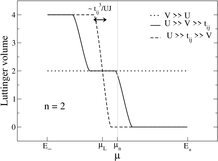
Figure 1: Schematic plot of the Luttinger volume [right-hand side of Eq. (1)] as a function of the chemical potential $\mu$. As $\mu$ is varied between the lower and upper edge of the gap, $E_{-}\leq\mu\leq E_{+}$, the density of electrons, $n=2$, remains fixed. While for a band insulator (dotted line) Luttinger’s theorem ($n$=Luttinger volume) is valid, this is not the case for strong interactions, where it is either fulfilled only for a single value of $\mu$, $\mu=\mu_{L}$, (dashed line) or only a limited range of chemical potentials (solid line). For fixed $n$ and $T\to 0$, the chemical potential takes the value $\mu_{n}=(E_{-}+E_{+})/2$ which coincides with $\mu_{L}$ only for a particle-hole symmetric system.

2.2 Finite bandwidth

It is convenient to discuss an expansion in the hopping $t_{ij}$ using the Greens function in real space, $G_{ij}(\omega)$, where $i$ and $j$ are site indices. To order $(t_{ij})^{2}$ only the local Greens function, $G_{ii}$ gets non-trivial corrections and therefore the self-energy remains local. The first correction to $G_{ij}$, $i\neq j$, which is not captured by (7), arises to order $(t_{ij})^{3}$ when an electron correlates the sites $i$ and $j$ by three hopping processes. Close to the poles of $G_{\text{loc}}(\omega)$, at $\omega+\mu\sim\pm\tilde{U}/2$, one has to resum perturbation theory in $t_{ij}$ to infinite order [to obtain e.g. the next correction to Eq. 8)] but this is not necessary in the center of the gap where the zeros of the Greens function are located.

Simple power-counting is not sufficient to get the precise dependence of the $(t_{ij})^{3}$ contribution on $U$ and $J$. In the limit $t_{ij}\ll J\ll U$, by solving a two-site system exactly we obtain $G_{ij}(\omega+\mu=0)\approx-12(t_{ij})^{3}/(U^{3}J)$. Comparing this to $G_{\text{loc}}(\omega)\approx(\omega+\mu)/(\tilde{U}/2)^{2}$ for small $\omega+\mu$, one finds after a Fourier transformation that the zeros of $G({\mathbf{p}},\omega)$ [and therefore also the poles of $\Sigma({\mathbf{p}},\omega)$] are approximately located at

$$\omega+\mu=E^{*}_{{\mathbf{p}}}\approx 3\sum_{i}\frac{(t_{i0})^{3}}{JU}\cos({\mathbf{p}}\cdot{\mathbf{r}}_{i})+O\!\left(\frac{(t_{ij})^{3}}{U^{2}},\frac{(t_{ij})^{4}}{UJ^{2}}\right)$$ (9)

where ${\mathbf{r}}_{i}$ is the vector pointing from site $0$ to site $i$. By definition, the Luttinger surface is given by $\mu=E^{*}_{{\mathbf{p}}}$ and its volume depends obviously strongly on the value of the chemical potential $\mu$ in a regime where $n=2=const.$ as is shown in Fig. 1. As discussed above, Luttinger’s sum rule is therefore violated.

Eq. (9) is consistent with results of Pairault, Sénéchal and Tremblay tremblay who performed a strong-coupling expansion for the single band Hubbard model [in combination with a resummation based on a continued-fraction expansion of $G({\mathbf{p}},\omega)$]. In their expression, the $J$ of Eq. (9) is replaced by the temperature $T$ reflecting the degeneracy of the strong-coupling ground-state of the single-band Hubbard model.

2.3 Canonical ensemble and position of the chemical potential

Within the Mott gap, there is precisely one value of the chemical potential $\mu=\mu_{L}$ where Luttinger’s sum rule, Eq. (1) is fulfilled (using again the parameters of Sec. 2.1 in this section). Furthermore, in a canonical ensemble (i.e. for fixed particle density $n$) the chemical potential has a well defined limiting value for $T\to 0$, $\mu_{n}=\lim_{T\to 0}\mu(n,T)$. Therefore the question arises, whether the Luttinger theorem is valid for a Mott insulator if a canonical ensemble is used where $\mu=\mu_{n}$ at $T=0$. Note that in a three-dimensional system, the electron density is fixed by the long-ranged Coulomb interaction and the background charge of the ions, therefore the chemical potential does take the value $\mu_{n}$ for $T\to 0$. Before showing that the Luttinger theorem is not valid in this case as generically $\mu_{L}\neq\mu_{n}$, one should first note that in the classical proofs of Luttinger’s theorem luttinger ; dzyaloshinskii always grand-canonical ensembles (fixed $\mu$) and never canonical ensembles (fixed $n$) are used and therefore there is little reason to believe that the Luttinger theorem is only valid for a canonical ensemble.

For a particle-hole symmetric situation (often studied in literature tsvelik1 ; tsvelik2 ; berthod ; stanescu ), $\mu_{n}$ and $\mu_{L}$ coincide by symmetry: the symmetry fixes both the value of $\mu$ and the position and shape of the Luttinger surface completely. Generically, particle-hole symmetry is not present. To show that $\mu_{n}$ and $\mu_{L}$ differ from each other in this case, we calculate both of them to leading order in the strong-coupling expansion.

In the canonical ensemble, the chemical potential in located precisely in the middle of the upper and lower edge of the gap, as the number of particle excitations $\propto e^{-(E_{+}-\mu)/T}$ has to be equal to the number of holes $\propto e^{-(\mu-E_{-})/T}$ for $T\to 0$ (see also Fig. 1). Using Eq. (8) one therefore obtains

$$\mu_{n}=\frac{E_{+}+E_{-}}{2}\approx\frac{\max[t_{\mathbf{p}}]+\min[t_{\mathbf{p}}]}{4}+O\!\left(\frac{t^{2}}{J},\frac{t^{2}}{U}\right)$$ (10)

This has to be compared to Eq. (9) which shows that $\mu_{L}=0+O[(t_{ij})^{3}/(UJ)]$. We have therefore proven that $\mu_{L}\neq\mu_{n}$ in the absence of particle-hole symmetry when $\max[t_{\mathbf{p}}]\neq-\min[t_{\mathbf{p}}]$. Accordingly, the Luttinger theorem is violated in the Mott insulating phase even for a canonical ensemble (in the absence of particle-hole symmetry).

Note that ambiguities in the definition of the chemical potential and in the frequency, where the Greens function matrix is evaluated within Luttinger’s theorem, are absent in systems where a Fermi surface exists. Adding to our insulating model (2) a further metallic band, which hybridizes only weakly with the two bands of the Mott insulating state, does not change any of our conclusions but fixes $\mu$ unambiguously even at $T=0$

2.4 Analysis of the proof

We will now investigate the question, which assumption underlying the proof of Luttinger’s theorem is not valid for a Mott insulator. The central step of the proof luttinger ; dzyaloshinskii (sketched in Appendix B) is to show that the integral

$$\int_{-\infty}^{\infty}\frac{d\omega}{2\pi}\,\Sigma({\mathbf{p}},i\omega)\frac{\partial}{\partial i\omega}G({\mathbf{p}},i\omega)$$ (11)

vanishes. The basic idea is to use that the self-energy can be written as a derivative of the Luttinger-Ward functional with respect to the Greens function such that the relevant integrand can be identified with a total derivative. Note that in (11) the integrand drops rapidly with $1/\omega^{2}$ for large frequencies and that (with the possible exception of the point $\omega=0$) no singularities are expected on the integration path along the imaginary axis. As Luttinger’s theorem is violated in the local limit, one can use the exact Greens function and self energy for $t_{ij}=0$, given by Eqs. (5) and (6), to calculate (e.g. by a trivial contour integration)

$$\int_{-\infty}^{\infty}\frac{d\omega}{2\pi}\,\Sigma_{\text{loc}}(i\omega)\frac{\partial}{\partial i\omega}G_{\text{loc}}(i\omega)=-\frac{1}{2}\,\text{sign}\,\mu$$ (12)

This well-behaved integral does not vanish, contrary to what is suggested by the proof of Luttinger’s theorem. Taking into account spin- and orbital summations, the factor $\pm 1/2$ explains the violation of Luttinger’s theorem by $\pm 2$ for $\mu\neq 0$ in the local limit.

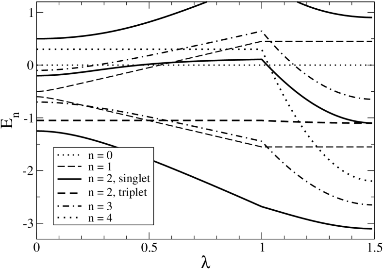
Figure 2: Evolution of the energy levels in the local limit, $t^{\alpha}_{ij}=0$, see Appendix A, as a function of a control parameter $\lambda$. For $\lambda=0$, the inter-orbital hybridization $V$ vanishes, $V=0$, and $U_{1}=1,U_{2}=1.5,\mu=0,J=0.2,\epsilon_{1}=-0.6,\epsilon_{2}=-0.5$. For $0\leq\lambda\leq 1$, $V=\lambda$ increases linearly with $\lambda$ and the interactions and $\mu$ stay constant. For $1\leq\lambda\leq 1.5$, $V=1$ is constant footnote but the interactions $U_{1}$, $U_{2}$ and $J$ drop proportional to $4(1.5-\lambda)^{2}$. For $\lambda=1.5$, the non-interacting system is characterized by two single-particle levels with energies $\frac{\epsilon_{1}+\epsilon_{2}}{2}\mp\sqrt{\left(\frac{\epsilon_{1}-\epsilon_{2}}{2}\right)^{2}+V^{2}}\approx-1.55$ and $0.45$. The groundstate is always a singlet with two electrons per site, $n=2$ well separated by a finite gap from all excited state. As there is no level crossing, the wave function evolves smoothly from a singlet made from localized electrons in two different bands (Mott insulator for small $\lambda$) to two electrons filling a single band (band insulator at $\lambda=1.5$). The finite gap to excited states guarantees that also in the presence of small but finite hopping $t^{\alpha}_{ij}$ two-orbital Mott- and band-insulator are adiabatically connected along the described path.

It is presently not clear, where precisely the problem is located in the arguments which try to show that (11) vanishes (see Appendix B). Despite the simple form of the self energy (6), bare perturbation theory is very singular for $\mu\neq 0$, $T=0$, as the density of the half-filled model, $n=2$, is reached only above a critical value of $U$. Inspection of the exact finite temperature Greens function in the local limit indeed shows divergencies with powers of $1/T$ to arbitrary order. One may therefore suspect that the replacement of Matsubara sums by integrals, i.e. the limit $T\to 0$, is problematic. Similarly, it may not be sufficient to show that (11) vanishes order by order in a skeleton expansion (see Appendix B) for such a non-perturbative problem. It is, however, interesting to remark, that the Luttinger-Ward functional can in principle be constructed non-perturbatively as pointed out by Potthoff pothoff who also emphasized in his paper that the proof of Luttinger’s theorem requires non-trivial assumptions on the regularity of the limit $T\to 0$. A more detailed discussion of assumptions underlying the proof can be found in Appendix B.

In Ref. altshuler , Altshuler et al. studied the question, to what extent Luttinger’s theorem applies to an antiferromagnetic metal if one insists to describe the system without explicitly breaking the symmetry. The authors found that in this situation the integral (11) does not vanish. In their case, the problem could be traced back to an anomaly (i.e. a contribution arising after the proper regularization of a divergence) which seems not to be the case for a Mott insulator with unique ground state studied here.

3 Adiabatic continuity

Based on the results discussed above, we will now investigate the crossover from a band- to a two-orbital Mott insulator (or Kondo insulator) with two electrons per unit cell, $n=2$. Note that we are not discussing the standard single-orbital Mott insulator with an odd number of electrons per unit cell, which in $d>1$ usually becomes magnetically ordered for $T=0$. For a band insulator Luttinger’s theorem is always trivially fulfilled and there is no Luttinger surface for any value of $\mu$. In contrast, we have shown that for $V,t_{ij}\ll U,J$, Luttinger’s theorem is violated for almost all values of $\mu$ within the gap. How does the crossover happen or is there a quantum phase transition between these two qualitatively different states? This question is answered by increasing $\sqrt{V^{2}+(\epsilon_{1}-\epsilon_{2})^{2}}$ in the model (2) in the trivial limit of small $t_{ij}$.

We first investigate the evolution of the ground state when changing the parameters smoothly starting from two coupled Mott insulators ($V=0$, $U_{1}=1,U_{2}=1.5,J=0.2$) and ending with a band insulator ($V=1$, $U_{i}=0,J=0$). For $t^{\alpha}_{ij}=0$, it is shown in Fig. 2 that on this adiabatic path the ground state remains a singlet always separated by a finite gap $\Delta$ from all excited states (as guaranteed by level repulsion). As the gap is finite, these conclusions hold also in the presence of a small but finite band-width, $t^{\alpha}_{ij}\neq 0$. This proves that there is no quantum-phase transition footnote , separating the two-orbital Mott insulator from the band insulator, instead there is just a smooth crossover (consistent with results in the literature, see e.g. Ref. monien2 ).

As an aside, we also note that it is generally believed that the magnetically ordered states of the particle-hole symmetric, half-filled one-band Hubbard model at small $U$ (spin-density wave insulator) and large $U$ (magnetically ordered Mott insulator) are adiabatically connected.

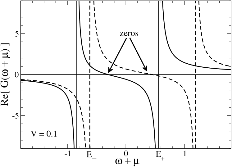
Figure 3: Both eigenvalues of the Greens-function matrix (solid and dashed) as a function of $\omega+\mu$ in the local limit $t^{\alpha}_{ij}=0$ for $V=0.1$, $U_{1}=1,U_{2}=1.5,J=0.2,\epsilon_{1}=-0.6,\epsilon_{2}=-0.5$ and a chemical potential within the gap, $E_{-}<\mu<E_{+}$. Both Greens functions change their sign within the gap for this value of $V$. Luttinger’s theorem holds only if the chemical potential is located between those zeros, see middle panel of Fig. 4.

To investigate the role of Luttinger’s theorem and the Luttinger surface as a function of the band splitting given by $\sqrt{V^{2}+(\epsilon_{2}-\epsilon_{1})^{2}}$, we first consider the effect of a potential $\Delta\epsilon=\epsilon_{2}-\epsilon_{1}$ which shifts the two bands relative to each other, $\epsilon_{1/2}=-U/2\pm\Delta\epsilon/2$, in the limit $V=t^{\alpha}_{ij}=0$ and $U_{1}=U_{2}=U$. The total charge gap is given by $U-\Delta\epsilon$ and the zeros of the Greens functions of the two orbitals split by $\Delta\epsilon$. For $\Delta\epsilon<U/2$, the two zeros remain within the gap. While Luttinger’s theorem is valid for $-\Delta\epsilon/2<\mu<\Delta\epsilon/2$, it is violated outside of this regime as is shown in Fig. 1 (for $t_{ij}=0$ the two jumps in the solid line become sharp step functions). For $U/2<\Delta\epsilon<U$, Luttinger’s sum rule (1) is valid for all values of $\mu$ within the gap but the system is still a Mott insulator in the sense that each of the two bands is singly occupied. For $\Delta\epsilon=U$, two levels cross and the ground-state wave-function changes in a first order transition which is an artifact of the limit $V=0$. Therefore this limit does not describe a smooth transition from a two-orbital Mott- to a band insulator, which can, however, be obtained by increasing the inter-orbital hybridization $V$.

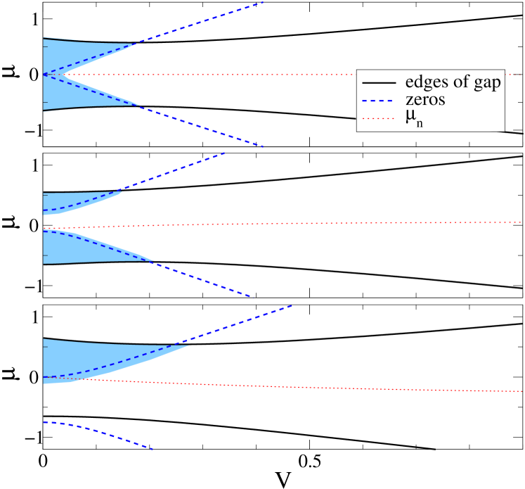
Figure 4: Crossover from the Mott insulator (small intra-orbital hybridization $V$) to a band insulator (large $V$). For a Mott insulator with a chemical potential in the shaded region, Luttinger’s theorem is violated (with the exception of the line $\mu=0$ in the upper panel). Luttinger’s theorem is, however, valid for a band insulator at large $V$. Solid lines denote the upper and lower band edge, the dashed lines the positions of the poles of the self-energy or equivalently of the zeros of the two Greens functions (see Fig. 3) obtained from the exact solution of the local model, $t^{\alpha}_{ij}=0$, sketched in Appendix A. In the plot the shaded region is not exactly delimited by the dashed lines to take schematically a small but finite hopping $t^{\alpha}_{ij}$ into account (c.f. Fig. 1). The dotted lines denote the position of the chemical potential for fixed particle number, $\mu_{n}=\lim_{T\to 0}\mu(n,T)$. Upper panel: particle-hole symmetric case with $U_{1}=U_{2}=1,\epsilon_{1}=\epsilon_{2}=-1/2,J=0.2,t^{\alpha}_{ij}=0$. Middle panel: same parameters as in Fig. 2. Lower panel: $U_{1}=1,U_{2}=2.5,\epsilon_{1}=-0.5,\epsilon_{2}=-2,J=0.2,t^{\alpha}_{ij}=0$.

Increasing $V$ has a very similar effect as increasing $\Delta\epsilon$ for $\Delta\epsilon<U$ as is shown in Figs. 3 and 4. The shaded regions in Fig. 4 indicate the range of chemical potentials where Luttinger’s theorem does not hold. As discussed above, also a finite but small hopping $t^{\alpha}_{ij}$ does not change the picture qualitatively (see Figs. 1 and 4).

4 Discussion

The main message of this paper is negative: Luttinger’s theorem in the form given by Eq. (1) is not valid in a Mott insulator and therefore the concept of a Luttinger surface (points in momentum space where the Greens function vanishes at $\omega=0$) seems not to be very useful — especially when compared to the much more powerful concept of a Fermi surface.

The basic argument is that a change of the chemical potential within the charge gap, $E_{-}<\mu<E_{+}$, just shifts the frequency argument of all Greens functions

$$G(\omega,{\mathbf{p}},\mu)=G(\omega+\mu,{\mathbf{p}})$$ (13)

If the Greens functions change their sign within the gap (as is the case for a Mott insulator), this implies that the sign of $G(\omega=0,{\mathbf{p}})$ and therefore the Luttinger volume depends on the arbitrary choice of $\mu$ while the density of electrons remains constant. We have also shown, that even in the canonical ensemble, when the chemical potential is fixed to $\lim_{T\to 0}\mu(n,T)$ by the particle density $n$, the Luttinger theorem is violated in the absence of particle-hole symmetry.

Often Luttinger’s theorem is stated in a different way: the volume enclosed by the Fermi surface (defined by poles rather than sign changes of the Greens functions) is given by the number of electrons per unit cell modulo $2$ (to take into account filled bands). For this case alternative proofs exist oshikawa ; praz which are based on Gauge invariance, topological arguments and the assumption that a Fermi liquid exists oshikawa or on particle-number conservation and an adiabatic connection of the interacting to the non-interacting metal praz . As we have consided only insulators with $n=2$, Luttinger’s theorem in this “Fermi-surface version” is trivially valid. Recently, Senthil, Sachdev and Vojta senthil argued that one can construct a situation where this is not the case. They considered a two-band model, where the first band is in its Mott insulating state such that it can be described by free spins. Senthil, Sachdev and Vojta then assumed that one can add strongly frustrating interactions between those spins such that the spins form a gapped spin liquid without breaking any symmetry. If the second band is weakly interacting, it will form a Fermi surface. As the spin-liquid is gapped, this state is robust against small perturbations like a finite coupling to the Fermi liquid of the second band, e.g. by a small $V$. In such a situation, the volume enclosed by the Fermi surface is given by the number of electrons in the second band $n_{2}$ rather than by the total number of electrons per unit cell, $n=1+n_{2}$. Combining this argument with the results of our paper, one realizes that in such a case both versions of Luttinger’s theorem are not valid (in the absence of particle-hole symmetry).

Luttinger’s theorem can also break down, if there is a finite imaginary part of the self energy at $\omega=0$. A large imaginary part has for example been observed in numerous studies of weakly doped Mott insulators at small, but finite temperatures, see e.g. Refs. haule , or in almost magnetic systems, e.g. Ref. vlik . Also in a slightly doped tJ model a violation of the Luttinger theorem has been observed in small systems prelovsek . It may be worthwhile to emphasize that the breakdown of Luttinger’s theorem discussed here is of different origin and probably unrelated.

Our analysis of Luttinger’s theorem, Eq. (1), appears to imply a qualitative difference between a band-insulator where it is valid and a two-orbital Mott insulator where it breaks down. Based on the “phase diagrams” of Fig. 4 one could define a “critical” hybridization $V_{c}$, e.g. by demanding that Luttinger’s theorem is valid for all $V\geq V_{c}$. We have, however, shown that at this “critical” hybridization, the ground-state energy (and essentially all observables with the exception of the Luttinger surface, the Luttinger volume and integral (11)) is analytic in $V-V_{c}$: no phase transition takes place. Instead there is a smooth crossover from a two-orbital ($n=2$) Mott- to a band-insulator. Recently, Konik, Rice and Tsvelik tsvelik2 investigated coupled Mott ladders constructing explicitly a state where simultaneously a Luttinger surface and several Fermi surfaces (due to small electron and hole pockets) are present. While we have not studied such a situation, in analogy to the results presented here, we speculate that the system studied in Ref. tsvelik2 is adiabatically connected to some non-interacting model where band-structure effects lead to the formation of particle and hole pockets.

While we have shown in this paper that band- and two-orbital Mott insulators can in principle be adiabatically connected, one should keep in mind that for many models there will be a series of first and/or second-order phase transitions to various metallic, insulating and/or symmetry broken states when the interactions are increased. The best studied case in this context is probably the ionic Hubbard model, see Refs. ionic ; ionic1 ; ionic2 ; ionic3 and references therein. Note, however, that the symmetries of this special model ensure ionic , that the Mott insulating phase has no spin gap in contrast to the case investigated in this paper.

For the future, it would be interesting to nail down more precisely under what conditions Luttinger’s theorem breaks down and which of the assumptions used in various proofs is most fragile. This is especially important, as Luttinger’s theorem can be a powerful tool to classify topologically different states of matter at least for metallic systems.

Appendix A: Spectrum of $H_{\text{loc}}^{i}$

The spectrum of the local Hamiltonian is given by the following energies: The empty site, $n=0$, has vanishing energy, $E_{0}=0$, while one obtains $E_{4}=2(\epsilon_{1}+\epsilon_{2})+U_{1}+U_{2}-4\mu$ for $n=4$. The energies of the four single-particle states, $n=1$, are $E_{1\pm}=\left(\frac{\epsilon_{1}+\epsilon_{2}}{2}\right)\pm\sqrt{\left(\frac{\epsilon_{1}-\epsilon_{2}}{2}\right)^{2}+V^{2}}-\mu$, while the 4 three-particle states have $E_{3\pm}=\epsilon_{1}+\epsilon_{2}+\left(\frac{\epsilon_{1}+\epsilon_{2}+U_{1}+U_{2}}{2}\right)\pm\sqrt{\left(\frac{\epsilon_{1}+U_{1}-\epsilon_{2}-U_{2}}{2}\right)^{2}+V^{2}}-3\mu$. The energy of the three $n=2$ triplet states is given by $E_{2t}=\epsilon_{1}+\epsilon_{2}+\frac{J}{4}-2\mu$. Furthermore there are three singlet states for $n=2$ with energies $E_{2s1}<E_{2s2}<E_{2s3}$ which can be determined by diagonalizing the $3\times 3$ matrix

$$\left(\begin{array}[]{ccc}2(\epsilon_{1}-\mu)+U_{1}&0&\sqrt{2}V\\ 0&2(\epsilon_{2}-\mu)+U_{2}&\sqrt{2}V\\ \sqrt{2}V&\sqrt{2}V&\epsilon_{1}+\epsilon_{2}-2\mu-3J/4\end{array}\right)$$ (A.1)

The analytic formulas for $E_{2si}$ can be obtained by solving a cubic equation. As they are not very instructive and rather long, they are not displayed here. We only note that level repulsion ensures that the three energies are not degenerate for $V\neq 0$.

The total size of the gap for charge excitations of the local model with ground-state $n=2$ is determined by $E_{1-}+E_{3-}-2E_{2s1}$. For $V=0$ it is for example given by $\frac{3}{2}J+\min[\epsilon_{1}+U_{1},\epsilon_{2}+U_{2}]-\max[\epsilon_{1},\epsilon_{2}]$.

From the eigenfunctions and eigenvalues of the Hamiltonian, one can easily obtain the Greens function.

Appendix B: A proof of Luttinger’s theorem

In this appendix we briefly sketch a version of the “proof” of Luttinger’s theorem. The first step is to insert $1=\frac{\partial}{\partial i\omega}(i\omega-\epsilon_{\mathbf{k}})$ in the expression for the density of electrons using imaginary frequencies dzyaloshinskii at $T=0$

$$n = \lim_{T\to 0,V\to\infty}\frac{2T}{V}\sum_{{\mathbf{p}}}\sum_{\omega_{n}}e^{i\omega_{n}\epsilon}G({\mathbf{p}},i\omega_{n})$$

$$= \int_{\omega{\mathbf{p}}}\frac{2e^{i\omega\epsilon}}{(2\pi)^{d+1}}G({\mathbf{p}},i\omega)\frac{\partial}{\partial i\omega}\left[G^{-1}({\mathbf{p}},i\omega)+\Sigma({\mathbf{p}},i\omega)\right]$$

$$= \frac{2}{(2\pi)^{d+1}}\int_{\omega{\mathbf{p}}}e^{i\omega\epsilon}\frac{\partial}{\partial i\omega}\ln[G^{-1}({\mathbf{p}},i\omega)]$$

$$-\frac{2}{(2\pi)^{d+1}}\int_{\omega{\mathbf{p}}}\int_{\omega}\Sigma({\mathbf{p}},i\omega)\frac{\partial}{\partial i\omega}G({\mathbf{p}},i\omega)$$

where $\int_{\omega{\mathbf{p}}}=\int_{-\infty}^{\infty}d\omega\int_{1^{st}\text{ BZ}}d^{d}{\mathbf{p}}$ describes the integration of frequencies along the imagninary axis and of momenta over the first Brillouin zone. For the last equation, we have performed a partial integration using that $\lim_{\omega\to\pm\infty}\Sigma({\mathbf{p}},i\omega)G({\mathbf{p}},i\omega)=0$. Using the usual analytic continuation arguments luttinger ; dzyaloshinskii and the vanishing of $\text{Im}\Sigma({\mathbf{p}},\omega=0)$ one can identify the first term in (Appendix B: A proof of Luttinger’s theorem) with the right-hand side of Eq. (1) [to keep the presentation simple, we omit the discussion of band indices luttinger ; dzyaloshinskii ]. Luttinger’s theorem is therefore valid if the second term in (Appendix B: A proof of Luttinger’s theorem) vanishes – which we have shown to be not the case for a generic Mott insulator.

Let us nevertheless try to “prove” it. The self energy can be obtained by varying the Luttinger-Ward functional luttinger $\Phi[G]$, $\Sigma({\mathbf{p}},i\omega)=\frac{\delta\Phi}{\delta G({\mathbf{p}},i\omega)}$. The Luttinger-Ward functional is given by the sum of all skeleton diagrams. By the equation $\Phi[G]=\int_{\omega{\mathbf{p}}}G({\mathbf{p}},i\omega){\Phi}_{G}({\mathbf{p}},i\omega)$ we define the functional ${\Phi}_{G}$ with

$$\Sigma({\mathbf{p}},i\omega)={\Phi}_{G}({\mathbf{p}},i\omega)+\int_{\omega^{\prime}{\mathbf{p}}^{\prime}}\!\!G({\mathbf{p}}^{\prime},i\omega^{\prime})\frac{\delta{\Phi}_{G}({\mathbf{p}}^{\prime},i\omega^{\prime})}{\delta G({\mathbf{p}},i\omega)}$$ (B.3)

Consider the following integral over a total derivative

$$0 = \int_{\omega{\mathbf{p}}}\frac{d}{di\omega}\left[G({\mathbf{p}},i\omega){\Phi}_{G}({\mathbf{p}},i\omega)\right]$$ (B.4)

By inspecting the self-energy style diagrams contributing to ${\Phi}_{G}({\mathbf{p}},i\omega)$ one realizes that a change of the external frequency $\omega$ can be absorbed by a change of the frequency of all internal lines and therefore

$$\frac{d}{di\omega}{\Phi}_{G}({\mathbf{p}},i\omega)=\int_{\omega^{\prime}{\mathbf{p}}^{\prime}}\frac{\delta{\Phi}_{G}({\mathbf{p}},i\omega)}{\delta G({\mathbf{p}}^{\prime},i\omega^{\prime})}\frac{d}{di\omega^{\prime}}G({\mathbf{p}}^{\prime},i\omega^{\prime})$$ (B.5)

One obtains

$$0 = \int_{\omega{\mathbf{p}}}\frac{d}{di\omega}\left[G({\mathbf{p}},i\omega){\Phi}_{G}({\mathbf{p}},i\omega)\right]$$ (B.6)

$$= \int_{\omega{\mathbf{p}}}\Bigl{[}{\Phi}_{G}\frac{d}{di\omega}G$$

$$+G\int_{\omega^{\prime}{\mathbf{p}}^{\prime}}\frac{\delta{\Phi}_{G}({\mathbf{p}},i\omega)}{\delta G({\mathbf{p}}^{\prime},i\omega^{\prime})}\frac{d}{di\omega^{\prime}}G({\mathbf{p}}^{\prime},i\omega^{\prime})\Bigr{]}$$

$$= \int_{\omega{\mathbf{p}}}\Sigma({\mathbf{p}},i\omega)\frac{\partial}{\partial i\omega}G({\mathbf{p}},i\omega)$$

where in the last step we have exchanged the $\omega,{\mathbf{p}}$ with the $\omega^{\prime},{\mathbf{p}}^{\prime}$ integration, renamed the variables and used Eq. (B.3). If all arguments leading to (B.6) are valid, then Luttinger’s theorem is proven by Eq. (Appendix B: A proof of Luttinger’s theorem).

However, in the main text, we have shown by an explicit example that (B.6) does not vanish. Therefore one of the steps in (B.6) is not valid for a Mott insulator. The first question is whether all integrals are well defined. This seems to be the case as for $\mu\neq 0$ there is no singularity on the imaginary axis and at least order by order in the skeleton expansion each term vanishes with $1/\omega^{2}$ for $\omega\to\pm\infty$. Also exchanging the order of integration is probably valid order by order in the skeleton expansion, as all integrals seem to be absolutely converget. As far as we can see, only two problems remain. Either the skeleton expansion used frequently above is highly singular or the problem is hidden in the limit $T\to 0$ and the use of integrals (instead of Matsubara sums) on the frequency axis and the use of derivatives with respect to frequencies was not correct. In the main text, it is argued that bare perturbation theory is very singular for $T\to 0$, indicating that the two problems are related.

References

- (1) I. Dzyaloshinskii, Phys. Rev. B 68, (2003) 85113 .
- (2) F. H. L. Essler and A. M. Tsvelik, Phys. Rev. B 65, 115117 (2002); F. H. L. Essler and A. M. Tsvelik, Phys. Rev. B 71, (2005) 195116.
- (3) R. M. Konik, T. M. Rice, A. M. Tsvelik, Phys. Rev. Lett. 96, (2006)086407.
- (4) K.-Y. Yang, T. M. Rice, and F.-C. Zhang, Phys. Rev. B 73, (2006) 174501.
- (5) T. D. Stanescu, P. W. Phillips and T-P. Choy, Physical Review B 75, (2007) 104503.
- (6) C. Berthod, T. Giarmarchi, S. Biermann, and A. Georges, Phys. Rev. Lett. 97, (2006) 136401.
- (7) J. Ortloff, M. Balzer, and M. Potthoff, Euro. Phys. J. B, 58, (2007) 37.
- (8) J. M Luttinger, Phys. Rev. 119, 1153 (1960); J. M Luttinger and J. C. Ward, Phys. Rev. 118, 1417 (1960).
- (9) S. Trebst, H. Monien, A. Grzesik, and M. Sigrist, Phys. Rev. B 73, 165101 (2006).
- (10) J. Hubbard, Proc. R. Soc. (London), Ser. A 276, 238 (1963).
- (11) W. Jones and N. H. March, Theoretical Solid State Physics, Vol. 1 (John Wiley & Sons, London, 1973).
- (12) S. Pairault, D. Sénéchal, and A.-M. S. Tremblay, Phys. Rev. Lett. 80, 5389 (1998).
- (13) M. Potthoff, Condens. Mat. Phys. 9, 557 (2006).
- (14) B. L. Altshuler, A. V. Chubukov, A. Dashevskii, A. M. Finkel’stein, and D. K. Morr, Europhys. Lett 41, 401 (1998).
- (15) The non-analytic kinks in Fig. 2 are a trivial artifact of the non-analytic dependence of the bare coupling constants on . They do therefore not signal a quantum phase transition.
- (16) G. Moeller, V. Dobrosavljević, and A. E. Ruckenstein, Phys. Rev. B 59, 6846 (1999); A. Fuhrmann, D. Heilmann, and H. Monien, Phys. Rev. B 73, (2006) 245118.
- (17) T. Senthil, S. Sachdev, and M. Vojta, Phys. Rev. Lett. 90, 216403 (2003).
- (18) M. Oshikawa, Phys. Rev. Lett. 84, 3370 (2000).
- (19) A. Praz, J. Feldman, H. Knörrer, and E. Trubowitz, Europhys. Lett. 72, 49 (2005).
- (20) M. Langer, J. Schmalian, S. Grabowski, and K. H. Bennemann, Phys. Rev. Lett. 75, 4508 (1995); C. Grober, R. Eder, and W. Hanke, Phys. Rev. B 62, 4336 (2000); K. Haule, A. Rosch, J. Kroha, and P. Wölfle, Phys. Rev. Lett. 89, 236402 (2002); Phys. Rev. B 68, 155119 (2003).
- (21) Y. M. Vlik, A.-M. S. Tremblay, J. Phys. I France. 7, 1309 (1997).
- (22) J. Kokalj, P. Prelovsek, Phys. Rev. B 75, (2007) 045111.
- (23) N. Nagaosa and J. Takimoto, J. Phys. Soc. of Japan 55, 2735 (1986).
- (24) M. Fabrizio, A. O. Gogolin, and A. A. Nersesyan, Phys. Rev. Lett. 83, 2014 (1999).
- (25) N. Paris, K. Bouadim, F. Hebert, G.G. Batrouni, and R.T. Scalettar, Phys. Rev. Lett. 98, (2007) 046403.
- (26) M. E. Torio, A. A. Aligia, G. I. Japaridze, and B. Normand, Phys. Rev. B 73, 115109 (2006).