Brueckner–Goldstone perturbation theory for the half-filled Hubbard model in infinite dimensions

Abstract

We use Brueckner–Goldstone perturbation theory to calculate the ground-state energy of the half-filled Hubbard model in infinite dimensions up to fourth order in the Hubbard interaction. We obtain the momentum distribution as a functional derivative of the ground-state energy with respect to the bare dispersion relation. The resulting expressions agree with those from Rayleigh–Schrödinger perturbation theory. Our results for the momentum distribution and the quasi-particle weight agree very well with those obtained earlier from Feynman–Dyson perturbation theory for the single-particle self-energy. We give the correct fourth-order coefficient in the ground-state energy which was not calculated accurately enough from Feynman–Dyson theory due to the insufficient accuracy of the data for the self-energy, and find a good agreement with recent estimates from Quantum Monte-Carlo calculations.

1 Introduction

The Hubbard model [1] is the ‘standard model’ for correlated electron systems [2]. It contains the essential ingredients for the description of itinerant electrons in a solid whose kinetic energy competes with their mutual Coulomb interaction. Since it contains very few parameters it provides an ideal development area and testing ground for (approximate) analytical and numerical techniques.

Despite its simplistic structure, the Hubbard model is very difficult to solve exactly. An exact solution via Bethe Ansatz exists in one spatial dimension, see Ref. [3] for a comprehensive account. Unfortunately, an exact solution is not possible in the limit of infinite dimension [4], and approximate numerical and analytical methods must be employed to solve the self-consistency equations of the resulting Dynamical Mean-Field Theory [5, 6]. Such approximate investigations must be supported by perturbatively controlled analytical calculations in the limits of weak and strong coupling. In this way, the quality of various approximation schemes was assessed in Refs. [7, 8, 9].

In Ref. [7], Feynman–Dyson perturbation theory was used to calculate the single-particle self-energy up to fourth order in the Hubbard interaction $U$. The ground-state energy $E_{0}(U)$ and the momentum distribution $n_{\sigma}(\epsilon(k);U)$ were obtained as moments of the spectral function which cannot be expressed in terms of a Taylor series in $U$. Therefore, Feynman–Dyson perturbation theory does not provide $E_{0}(U)$ and $n_{\sigma}(\epsilon(k);U)$ in form of a Taylor series in $U$. The coefficient of the fourth-order term of the ground-state energy as determined in Ref. [7] does not agree with results from recent Quantum Monte-Carlo investigations [10].

In this work we employ the Brueckner–Goldstone perturbation expansion to the Hubbard model in infinite dimensions. This (stationary) perturbation theory has the advantage that it provides $E_{0}(U)$ and $n_{\sigma}(\epsilon(k);U)$ as a Taylor series in $U$. As a result, the Brueckner–Goldstone approach requires less numerical effort to calculate $E_{0}(U)$ and $n_{\sigma}(\epsilon(k);U)$ than the Feynman–Dyson perturbation theory and, thus, gives more accurate results for the same amount of computational effort. An exception is the quasi-particle weight $Z(U)$ which is algebraically related to the slope of the real part of the self-energy at the Fermi energy and gives the size of the discontinuity of the momentum distribution at the Fermi energy. Therefore, we can directly compare $Z(U)$ from Feynman–Dyson perturbation theory in Ref. [7] with the corresponding expression from Brueckner–Goldstone expansion in this work.

Our work is organized as follows. In Sect. 2, we introduce the Hubbard model and our physical quantities of interest. In Sect. 3, we use Brueckner–Goldstone perturbation theory to calculate the ground-state energy of the Hubbard model in infinite dimensions up to and including fourth order in the Hubbard interaction. We find that the fourth-order coefficient quoted in Ref. [7] is indeed incorrect. The correct value agrees with recent Quantum Monte-Carlo data [10]. In Sect. 4, we calculate the momentum distribution starting from the Brueckner–Goldstone expressions for the ground-state energy. In infinite dimensions, $n_{\sigma}(\epsilon(k);U)$ can be expressed as a functional derivative of the ground-state energy with respect to the bare dispersion relation $\epsilon(k)$. Our results for the momentum distribution and the quasi-particle weight agree very well with those obtained previously from Feynman–Dyson perturbation theory [7]. We conclude in Sect. 5.

2 Physical quantities

2.1 Hamilton Operator

We investigate spin-1/2 electrons which move on a $d$-dimensional lattice with $L$ lattice sites. The corresponding operator for the kinetic energy reads

$$\hat{T}=\sum_{l,m;\sigma}t(l-m)\hat{c}_{l,\sigma}^{+}\hat{c}_{m,\sigma}^{\phantom{+}}\;,$$ (1)

where $\hat{c}^{+}_{l,\sigma}$, $\hat{c}_{l,\sigma}$ are creation and annihilation operators for electrons with spin $\sigma=\uparrow,\downarrow$ on site $l$. The thermodynamical limit, $L\to\infty$, and the limit of infinite dimensions, $d\to\infty$, are implicitly understood henceforth.

The kinetic energy is diagonal in momentum space

$$\hat{T}=\sum_{k,\sigma}\epsilon(k)\hat{c}_{k,\sigma}^{+}\hat{c}_{k,\sigma}^{\phantom{+}}$$ (2)

with the dispersion relation

$$\epsilon(k)=\sum_{r}t(r)e^{-{\rm i}kr}\;.$$ (3)

Note that all momenta are taken from the first Brillouin zone. The ground state of the kinetic energy is the Fermi-sea $|{\rm FS}\rangle$,

$$|{\rm FS}\rangle=\prod_{k,\sigma;\epsilon(k)\leq E_{\rm F}}\hat{c}_{k,\sigma}^{+}|{\rm vacuum}\rangle\;,$$ (4)

where $E_{\rm F}$ is the Fermi energy.

Later we shall work with a semi-circular density of states for non-interacting electrons,

$$D_{0}(\epsilon)\equiv\frac{1}{L}\sum_{k}\delta(\epsilon-\epsilon(k))=\frac{2}{\pi W}\sqrt{4-\left(\frac{4\epsilon}{W}\right)^{2}\,}\Theta\left(\left(W/2\right)^{2}-\epsilon^{2})\right),$$ (5)

where $W\equiv 4t$ is the bandwidth and $\Theta(x)$ denotes the Heaviside step function. This density of states is realized for a Bethe lattice with infinite connectivity [11]. In the following, we set $t\equiv 1$ as our energy unit.

The electron-electron interaction is taken to be purely on-site with strength $U$,

$$\hat{H}_{1}=U\hat{D}=U\sum_{l}\left(\hat{n}_{l,\uparrow}-\frac{1}{2}\right)\left(\hat{n}_{l,\downarrow}-\frac{1}{2}\right)\;,$$ (6)

where $\hat{n}_{l,\sigma}=\hat{c}^{+}_{l,\sigma}\hat{c}_{l,\sigma}^{\phantom{+}}$ is the local density operator at site $l$ for spin $\sigma$. The Hubbard Hamiltonian then becomes

$$\hat{H}=\hat{T}+\hat{H}_{1}=\hat{T}+U\hat{D}\;.$$ (7)

The Hamiltonian is invariant under SU(2) spin transformations so that the total spin is a good quantum number. We demand that the model exhibits particle-hole symmetry on bipartite lattices, i.e., $\hat{H}$ is assumed to be invariant under the transformation

$${\rm PH}:\qquad\hat{c}_{l,\sigma}^{+}\mapsto(-1)^{l}\hat{c}_{l,\sigma}\quad;\quad\hat{c}_{l,\sigma}\mapsto(-1)^{l}\hat{c}_{l,\sigma}^{+}\;,$$ (8)

where $(-1)^{l}=1$ on the $A$-sites and $(-1)^{l}=-1$ on the $B$-sites. Therefore, the model is altogether SO(4)-symmetric [3]. This implies that there exists a nesting vector $Q$ such that $\exp({\rm i}Ql)=(-1)^{l}$ and, therefore, $\epsilon(k+Q)=-\epsilon(k)$. We consider exclusively a half-filled band where the number of electrons $N=2N_{\sigma}$ equals the number of lattice sites $L$ so that we may set the Fermi energy to zero, $E_{\rm F}=0$.

2.2 Ground-state energy, momentum distribution and quasi-particle weight

Let $|0\rangle$ be the normalized exact ground state of $\hat{H}$. As a consequence of the particle-hole symmetry (8), the ground-state energy of the Hubbard Hamiltonian (7) at half band-filling is an even function of $U$ [3],

$$E_{0}(U)\equiv\langle 0|\hat{H}|0\rangle=E_{0}(-U)\;.$$ (9)

Therefore, the Taylor expansion of $E_{0}(U)$ contains even powers in $U$ only,

$$E_{0}(U)=E_{0}^{(0)}+U^{2}E_{0}^{(2)}+U^{4}E_{0}^{(4)}+\ldots\;.$$ (10)

For a semi-circular density of states, the average kinetic energy of the half-filled Fermi sea is readily calculated as

$$\frac{E_{0}^{(0)}}{L}\equiv 2\int_{-2}^{0}{\rm d}\epsilon D_{0}(\epsilon)\epsilon=-\frac{8}{3\pi}\;.$$ (11)

We shall calculate the coefficients to second and fourth order with the help of Brueckner–Goldstone perturbation theory in section 3.

The momentum distribution is defined by

$$n_{k,\sigma}(U)=\langle 0|\frac{1}{L}\sum_{l,m}e^{{\rm i}(l-m)k}\hat{c}_{l,\sigma}^{+}\hat{c}_{m,\sigma}^{\phantom{+}}|0\rangle\;.$$ (12)

In the limit of infinite dimensions, the momentum distribution depends on the momentum $k$ only through the dispersion relation $\epsilon(k)$ [2]. Therefore, we write $n_{k,\sigma}(U)\equiv n_{\sigma}(\epsilon(k);U)\equiv n_{\sigma}(\epsilon;U)$. The particle-hole transformation (8) ensures that

$$n_{\sigma}(\epsilon;U)=n_{\sigma}(\epsilon;-U)=1-n_{\sigma}(-\epsilon;U)\;.$$ (13)

Therefore, the Taylor expansion of $n_{\sigma}(\epsilon;U)$ contains even powers in $U$ only,

$$n_{\sigma}(\epsilon;U)=n_{\sigma}^{(0)}(\epsilon)+U^{2}n_{\sigma}^{(2)}(\epsilon)+U^{4}n_{\sigma}^{(4)}(\epsilon)+\ldots\;,$$ (14)

and we may restrict ourselves to $\epsilon>0$ in the calculation of the momentum distribution. The leading term in (14) is the momentum distribution for free fermions,

$$n_{\sigma}^{(0)}(\epsilon)=\Theta(4-\epsilon^{2})\Theta(-\epsilon)=\left\{\begin{array}[]{lcl}1&\hbox{for}&-2\leq\epsilon\leq 0\\ 0&\hbox{for}&\hphantom{-}0<\epsilon\leq 2\end{array}\right.\;.$$ (15)

We shall calculate the coefficients to second and fourth order with the help of Brueckner–Goldstone perturbation theory in section 4.

The discontinuity of the momentum distribution at the Fermi energy $E_{\rm F}=0$ is of particular interest because it gives the quasi-particle weight $Z(U)$. By definition,

$$Z(U)=n_{\sigma}(\epsilon=0^{-})-n_{\sigma}(\epsilon=0^{+})=1-2n_{\sigma}(\epsilon=0^{+})\;,$$ (16)

and the Taylor expansion reads

$$Z(U)=1+Z^{(2)}\frac{U^{2}}{t^{2}}+Z^{(4)}\frac{U^{4}}{t^{4}}\ldots\;.$$ (17)

In infinite dimensions, this quantity is related to the slope of the self-energy at the Fermi energy via

$$Z(U)=\left[1-\left.\frac{\partial{\rm Re}\Sigma(\omega;U)}{\partial\omega}\right|_{\omega=0}\right]^{-1}\;.$$ (18)

The self-energy $\Sigma(\omega;U)$ was calculated in [7] to fourth order in the Hubbard interaction. Therefore, we can directly compare our results for $Z(U)$ from Brueckner–Goldstone perturbation theory with those from Feynman–Dyson perturbation theory.

3 Ground-state energy

According to Brueckner–Goldstone perturbation theory [12, 13], the ground-state energy can be expressed as a power series in the interaction strength,

$$E_{0}-E_{0}^{(0)}=\langle{\rm FS}|\hat{H}_{1}\sum_{j=0}^{\infty}\left((E_{0}^{(0)}-\hat{T})^{-1}\hat{H}_{1}\right)^{j}|{\rm FS}\rangle_{\rm c}\;.$$ (19)

Here, the subscript ‘c’ indicates that only connected diagrams must be included in a diagrammatic formulation of the theory. Note that no diagrams with Hartree bubbles appear because they have been subtracted explicitly in the definition of $\hat{H}_{1}$. Moreover, due to particle-hole symmetry, only odd $j$ contribute to the series in (19).

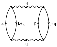
Figure 1: Second-order Goldstone diagram.

3.1 Second order

The ground-state energy to second order is given by

$$E_{0}^{(2)}=\langle{\rm FS}|\hat{D}(E_{0}^{(0)}-\hat{T})^{-1}\hat{D}|{\rm FS}\rangle_{\rm c}\;,$$ (20)

to which only a single diagram contributes, see Fig. 1. In this figure, a line with a down-going arrow indicates a particle line, a line with an up-going arrow represents a hole line, and a wiggly line indicates the transferred momentum $q$. Note that $q\neq 0$ applies because we can write the interaction in momentum space as

$$\hat{D}=\frac{1}{L}\sum_{k,p}\sum_{q\neq 0}\hat{c}_{k+q,\uparrow}^{+}\hat{c}_{k,\uparrow}^{\phantom{+}}\hat{c}_{p-q,\downarrow}^{+}\hat{c}_{p,\downarrow}^{\phantom{+}}\;.$$ (21)

The diagram is readily calculated from the Goldstone diagram rules,

$$\frac{E_{0}^{(2)}}{L} = -\left(\frac{1}{L}\right)^{3}\sum_{k,p}\sum_{q\neq 0}[(1-n_{\sigma}^{(0)}(\epsilon(k+q))]n_{\sigma}^{(0)}(\epsilon(k))$$ (22)

$$\hphantom{-\left(\frac{1}{L}\right)^{3}\sum_{k,p}\sum_{q\neq 0}}\times\frac{[1-n_{\sigma}^{(0)}(\epsilon(p-q))]n_{\sigma}^{(0)}(\epsilon(p))}{\epsilon(k+q)-\epsilon(k)+\epsilon(p-q)-\epsilon(p)}\;.$$

The diagram was evaluated in one, two and three dimensions in Ref. [13].

To make progress in the limit of infinite dimensions [4], we introduce the joint density of states via

$$D_{q}(\epsilon_{1},\epsilon_{2})=\frac{1}{L}\sum_{k}\delta(\epsilon_{1}-\epsilon(k+q))\delta(\epsilon_{2}-\epsilon(k))\;,$$ (23)

and write

$$\frac{E_{0}^{(2)}}{L} = -\!\!\int{\rm d}\epsilon_{1}{\rm d}\epsilon_{2}{\rm d}\epsilon_{3}{\rm d}\epsilon_{4}\frac{[(1-n_{\sigma}^{(0)}(\epsilon_{1})]n_{\sigma}^{(0)}(\epsilon_{2})[(1-n_{\sigma}^{(0)}(\epsilon_{3})]n_{\sigma}^{(0)}(\epsilon_{4})}{\epsilon_{1}-\epsilon_{2}+\epsilon_{3}-\epsilon_{4}}$$ (24)

$$\hphantom{-\int{\rm d}\epsilon_{1}{\rm d}\epsilon_{2}{\rm d}\epsilon_{3}{\rm d}\epsilon_{4}}\frac{1}{L}\sum_{q\neq 0}D_{q}(\epsilon_{1},\epsilon_{2})D_{-q}(\epsilon_{3},\epsilon_{4})\;.$$

We note that the joint density of states factorizes in infinite dimensions [2],

$$D_{q}(\epsilon_{1},\epsilon_{2})=D_{0}(\epsilon_{1})D_{0}(\epsilon_{2})\qquad\hbox{for `almost all'~{}$q$.}$$ (25)

Therefore, the contribution of the $\uparrow$ electrons and the $\downarrow$ electrons separate. This amounts to the statement that the second-order diagram is a ‘local diagram’, i.e., the momentum conservation at the vertices can be ignored. With the help of the Feynman trick

$$\frac{1}{x}=\int_{0}^{\infty}{\rm d}\lambda e^{-\lambda x}\quad\hbox{for}\quad x>0$$ (26)

we write

$$\frac{E_{0}^{(2)}}{L}=-\int_{0}^{\infty}{\rm d}\lambda s_{\uparrow}(\lambda)s_{\downarrow}(\lambda)\;,$$ (27)

where

$$s_{\sigma}(\lambda)=F_{\rm p}(\lambda)F_{\rm h}(\lambda)$$ (28)

with the particle and hole contributions

$$F_{\rm p}(\lambda) = \frac{1}{L}\sum_{p,\epsilon(p)>0}e^{-\lambda\epsilon(p)}=\int_{0}^{\infty}{\rm d}\epsilon D_{0}(\epsilon)e^{-\lambda\epsilon}\;,$$ (29)

$$F_{\rm h}(\lambda) = \frac{1}{L}\sum_{p,\epsilon(p)\leq 0}e^{\lambda\epsilon(p)}=\int_{-\infty}^{0}{\rm d}\epsilon D_{0}(\epsilon)e^{\lambda\epsilon}\;.$$ (30)

For the calculation of the ground-state energy we may set $F_{\rm p}(\lambda)=F_{\rm h}(\lambda)\equiv F(\lambda)$ and we arrive at the final result [4]

$$\frac{E_{0}^{(2)}}{L}=-\int_{0}^{\infty}{\rm d}\lambda[F(\lambda)]^{4}\;.$$ (31)

For the semi-circular density of states we find the numerical value $E_{0}^{(2)}/L=-0.020866148383$.

3.2 Fourth order

The calculation of the ground-state energy to fourth order requires the evaluation of

$$E_{0}^{(4)}=\langle{\rm FS}|\hat{D}(E_{0}^{(0)}-\hat{T})^{-1}\hat{D}(E_{0}^{(0)}-\hat{T})^{-1}\hat{D}(E_{0}^{(0)}-\hat{T})^{-1}\hat{D}|{\rm FS}\rangle_{\rm c}\;.$$ (32)

The Goldstone diagrams now contain four vertices and the nine diagram parts for one spin species are shown in Fig. 2, together with their sign which results from the fermionic commutation relations after the application of Wick’s theorem. Note that the diagrams within the first, second, and third line are particle-hole symmetric to each other, i.e., $(a)\rightleftharpoons(g)$, $(b)\rightleftharpoons(f)$, and $(e)\rightleftharpoons(h)$. The diagrams $(c)$, $(d)$ and $(i)$ map onto each other under a particle-hole transformation.

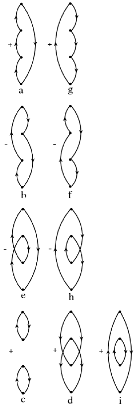
Figure 2: Diagram parts for one spin species for the fourth-order Goldstone diagrams.

In order to generate all possible diagrams, we draw all 81 possible pairs of diagrams from $(a)_{\uparrow}\times(a)_{\downarrow}$, $(a)_{\uparrow}\times(b)_{\downarrow}$, …, to $(i)_{\uparrow}\times(i)_{\downarrow}$, and connect all vertices with horizontal interaction lines. As an example, the diagram $(a)_{\uparrow}\times(i)_{\downarrow}$ is shown in Fig. 3.

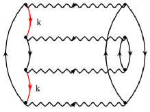
Figure 3: Fourth-order Goldstone diagram $(a)_{\sigma}\times(i)_{-\sigma}$ with ‘self-energy insertion’.

Not all of the 81 diagrams are connected, namely, the diagrams $(c)_{\uparrow}\times(c)_{\downarrow}$, $(d)_{\uparrow}\times(d)_{\downarrow}$, and $(i)_{\uparrow}\times(i)_{\downarrow}$ are disconnected and drop out. Moreover, the diagrams $(a)_{\sigma}\times(c)_{-\sigma}$, $(b)_{\sigma}\times(c)_{-\sigma}$, $(g)_{\sigma}\times(c)_{-\sigma}$, and $(f)_{\sigma}\times(c)_{-\sigma}$ as well as $(b)_{\sigma}\times(d)_{-\sigma}$ and $(f)_{\sigma}\times(d)_{-\sigma}$ contain a hole-line and a particle-line with the same momentum and therefore vanish due to the factor $n_{\sigma}^{(0)}(\epsilon)(1-n_{\sigma}^{(0)}(\epsilon))$. Nevertheless, it is quite tedious to work out the remaining 66 diagrams even when the spin-flip symmetry is employed.

We proceed differently. If all 66 diagrams were local diagrams, we could ignore the momentum conservation at the vertices as in the case of the second-order diagram in Sect. 3.1. The contribution of all non-vanishing connected diagrams would be

$$\frac{\widetilde{E}_{0}^{(4)}}{L} = (-1)^{3}\int_{0}^{\infty}{\rm d}\lambda_{1}\int_{0}^{\infty}{\rm d}\lambda_{2}\int_{0}^{\infty}{\rm d}\lambda_{3}$$ (33)

$$\hphantom{(-1)^{3}\int_{0}^{\infty}{\rm d}\lambda_{1}}\left[a+b+c+d+e+f+g+h+i\right]^{2}$$

$$\hphantom{(-1)^{3}\int_{0}^{\infty}{\rm d}\lambda_{1}}-\left[c^{2}+d^{2}+e^{2}\right]$$

$$\hphantom{(-1)^{3}\int_{0}^{\infty}{\rm d}\lambda_{1}}-2\left[a+b+g+f\right]c-2\left[b+f\right]d\;,$$

where all functions in the integrand are functions of $\lambda_{1},\lambda_{2},\lambda_{3}$. Explicitly, we have

$$a(\lambda_{1},\lambda_{2},\lambda_{3}) = F_{\rm p}(\lambda_{1}+\lambda_{2}+\lambda_{3})F_{\rm h}(\lambda_{1})F_{\rm h}(\lambda_{2})F_{\rm h}(\lambda_{3})\;,$$ (34)

$$g(\lambda_{1},\lambda_{2},\lambda_{3}) = F_{\rm h}(\lambda_{1}+\lambda_{2}+\lambda_{3})F_{\rm p}(\lambda_{1})F_{\rm p}(\lambda_{2})F_{\rm p}(\lambda_{3})\;,$$ (35)

$$b(\lambda_{1},\lambda_{2},\lambda_{3}) = -F_{\rm p}(\lambda_{1})F_{\rm h}(\lambda_{3})F_{\rm p}(\lambda_{2}+\lambda_{3})F_{\rm h}(\lambda_{1}+\lambda_{2})\;,$$ (36)

$$f(\lambda_{1},\lambda_{2},\lambda_{3}) = -F_{\rm h}(\lambda_{1})F_{\rm p}(\lambda_{3})F_{\rm h}(\lambda_{2}+\lambda_{3})F_{\rm p}(\lambda_{1}+\lambda_{2})\;,$$ (37)

$$e(\lambda_{1},\lambda_{2},\lambda_{3}) = -F_{\rm p}(\lambda_{1}+\lambda_{2}+\lambda_{3})F_{\rm h}(\lambda_{1}+\lambda_{2})F_{\rm p}(\lambda_{2})F_{\rm h}(\lambda_{2}+\lambda_{3})\;,$$

$$h(\lambda_{1},\lambda_{2},\lambda_{3}) = -F_{\rm h}(\lambda_{1}+\lambda_{2}+\lambda_{3})F_{\rm p}(\lambda_{1}+\lambda_{2})F_{\rm h}(\lambda_{2})F_{\rm p}(\lambda_{2}+\lambda_{3})\;,$$

$$c(\lambda_{1},\lambda_{2},\lambda_{3}) = F_{\rm h}(\lambda_{1})F_{\rm p}(\lambda_{1})F_{\rm h}(\lambda_{3})F_{\rm p}(\lambda_{3})\;,$$ (40)

$$d(\lambda_{1},\lambda_{2},\lambda_{3}) = F_{\rm p}(\lambda_{1}+\lambda_{2})F_{\rm h}(\lambda_{1}+\lambda_{2})F_{\rm p}(\lambda_{2}+\lambda_{3})F_{\rm h}(\lambda_{2}+\lambda_{3})\;,$$

$$i(\lambda_{1},\lambda_{2},\lambda_{3}) = F_{\rm p}(\lambda_{1}+\lambda_{2}+\lambda_{3})F_{\rm h}(\lambda_{1}+\lambda_{2}+\lambda_{3})F_{\rm p}(\lambda_{2})F_{\rm h}(\lambda_{2})\;.$$

Eq. (33) gives the fourth-order ground-state energy for the Wolff model [14] where the Hubbard interaction acts only on one site.

However, even in infinite dimensions not all diagrams are local diagrams. First, there are diagrams with a ‘self-energy insertion’, namely $(a)_{\sigma}\times(i)_{-\sigma}$ as shown in Fig. 3, and its particle-hole transformed counterpart $(g)_{\sigma}\times(i)_{-\sigma}$. As indicated in the figure, two hole lines have the same momentum. Therefore, the contribution of these diagrams is

$$A=2(-1)^{3}\int_{0}^{\infty}{\rm d}\lambda_{1}\int_{0}^{\infty}{\rm d}\lambda_{2}\int_{0}^{\infty}{\rm d}\lambda_{3}\left[a_{2}+g_{2}\right]i$$ (43)

with

$$a_{2}(\lambda_{1},\lambda_{2},\lambda_{3}) = F_{\rm p}(\lambda_{1}+\lambda_{2}+\lambda_{3})F_{\rm h}(\lambda_{1}+\lambda_{3})F_{\rm h}(\lambda_{2})\;,$$ (44)

$$g_{2}(\lambda_{1},\lambda_{2},\lambda_{3}) = F_{\rm h}(\lambda_{1}+\lambda_{2}+\lambda_{3})F_{\rm p}(\lambda_{1}+\lambda_{3})F_{\rm p}(\lambda_{2})\;.$$ (45)

The contribution $A$ replaces the terms $2(a+g)i$ in (33).

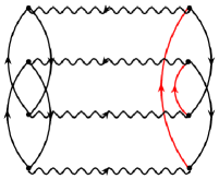
Figure 4: ‘Pauli-forbidden’ fourth-order Goldstone diagram $(d)_{\sigma}\times(h)_{-\sigma}$. The two hole-lines in the right part of the figure carry the same momentum.

Second, different contributions result from the ‘Pauli-forbidden diagrams’. The first class of Pauli-forbidden diagrams is generated by $(d)_{\sigma}\times(h)_{-\sigma}$, as shown in Fig. 4, and its particle-hole transformed counterpart $(d)_{\sigma}\times(e)_{-\sigma}$. As shown in the figure, there appear to be two holes with the same momentum in an intermediate state. Recall that Goldstone diagrams which appear to violate the exclusion principle must be retained [12]. The corresponding contribution is

$$B=2(-1)^{3}\int_{0}^{\infty}{\rm d}\lambda_{1}\int_{0}^{\infty}{\rm d}\lambda_{2}\int_{0}^{\infty}{\rm d}\lambda_{3}\left[h_{2}+e_{2}\right]d$$ (46)

with

$$h_{2}(\lambda_{1},\lambda_{2},\lambda_{3}) = -F_{\rm h}(\lambda_{1}+2\lambda_{2}+\lambda_{3})F_{\rm p}(\lambda_{2}+\lambda_{3})F_{\rm p}(\lambda_{1}+\lambda_{2})\;,$$ (47)

$$e_{2}(\lambda_{1},\lambda_{2},\lambda_{3}) = -F_{\rm p}(\lambda_{1}+2\lambda_{2}+\lambda_{3})F_{\rm h}(\lambda_{2}+\lambda_{3})F_{\rm h}(\lambda_{1}+\lambda_{2})\;.$$ (48)

The contribution $B$ replaces the terms $2(h+e)d$ in (33).

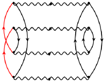
Figure 5: ‘Pauli-forbidden’ fourth-order Goldstone diagram $(e)_{\sigma}\times(i)_{-\sigma}$. The two hole lines in the left part of the figure carry the same momentum.

The second class of Pauli-forbidden diagrams results from $(e)_{\sigma}\times(i)_{-\sigma}$, as shown in Fig. 5, and its particle-hole transformed counterpart $(h)_{\sigma}\times(i)_{-\sigma}$, where again two holes have the same momentum in an intermediate state. The corresponding contribution is

$$C=2(-1)^{3}\int_{0}^{\infty}{\rm d}\lambda_{1}\int_{0}^{\infty}{\rm d}\lambda_{2}\int_{0}^{\infty}{\rm d}\lambda_{3}\left[h_{4}+e_{4}\right]i$$ (49)

with

$$h_{4}(\lambda_{1},\lambda_{2},\lambda_{3}) = -F_{\rm h}(\lambda_{1}+\lambda_{2}+\lambda_{3})F_{\rm p}(\lambda_{1}+2\lambda_{2}+\lambda_{3})F_{\rm h}(\lambda_{2})\;,$$ (50)

$$e_{4}(\lambda_{1},\lambda_{2},\lambda_{3}) = -F_{\rm p}(\lambda_{1}+\lambda_{2}+\lambda_{3})F_{\rm h}(\lambda_{1}+2\lambda_{2}+\lambda_{3})F_{\rm p}(\lambda_{2})\;.$$ (51)

The contribution $C$ replaces the terms $2(h+e)i$ in (33).

Altogether, the ground-state energy to fourth order becomes

$$\frac{E_{0}^{(4)}}{L} = \frac{\widetilde{E}_{0}^{(4)}}{L}+A+B+C$$

$$-\int_{0}^{\infty}{\rm d}\lambda_{1}\int_{0}^{\infty}{\rm d}\lambda_{2}\int_{0}^{\infty}{\rm d}\lambda_{3}\left[2(a+g+h+e)i+2(h+e)d\right]\;.$$

The single three-fold integral can be carried out on a PC after a suitable representation of $F(\lambda)$ in (29) has been found, e.g., in terms of a power series for small and large arguments.

For the semi-circular density of states, we find the fairly small value $E_{0}^{(4)}/L=7.2475\cdot 10^{-6}$. Thus, the ground-state energy of the Hubbard model on a Bethe lattice with infinite connectivity reads

$$\frac{E_{0}(U)}{L} = -\frac{8t}{3\pi}-0.02086614838\frac{U^{2}}{t}+0.0000072475\frac{U^{4}}{t^{3}}+{\cal O}\left(\frac{U^{6}}{t^{5}}\right)$$

$$= -\frac{2W}{3\pi}-0.08346459\frac{U^{2}}{W}+0.00046384\frac{U^{4}}{W^{3}}+{\cal O}\left(\frac{U^{6}}{W^{5}}\right)\;,$$

up to fourth order in the interaction ($W=4t$ is the bandwidth). Similar to the situation in the symmetric single-impurity Anderson model [15], the coefficient to fourth order is very small. For this reason, it is very difficult to extract it from the moments of the single-particle Green function. In fact, in Ref. [7], the single-particle self-energy as a function of frequency was not calculated accurately enough to give the correct sign of the fourth-order coefficient. The correct value given in (LABEL:eq:energyfinal) agrees very well with latest data from Quantum Monte-Carlo calculations [10], $E_{0}^{(4),{\rm QMC}}/L=(5\pm 2)\cdot 10^{-4}$.

4 Momentum distribution and quasi-particle weight

As shown in Sect. 3, in infinite dimensions the ground-state energy can be cast into the form

$$E_{0}=\sum_{k}\epsilon(k)n(\epsilon(k))+\langle 0|\hat{H}_{1}|0\rangle\;,$$ (54)

where $n(\epsilon)=2n_{\sigma}(\epsilon(k))$ is the spin-summed momentum distribution. This equation shows that we can obtain $n_{\sigma}(\epsilon(k))$ as a functional derivative of the ground-state energy,

$$n_{\sigma}(\epsilon(k))=\frac{1}{2}\frac{\delta E_{0}}{\delta\epsilon(k)}\;.$$ (55)

This is indeed correct to lowest order, as seen from

$$E_{0}^{(0)}=2\sum_{p;-2\leq\epsilon(p)\leq 0}\epsilon(p)\;,$$ (56)

which, together with (55), leads to (15).

4.1 Second order

In the limit of infinite dimensions, the ground-state energy can be written as a function of $F_{{\rm p},{\rm h}}(\lambda)$, see eq. (29). For $\epsilon(k)>0$, we need

$$\frac{\delta F_{\rm p}(\lambda)}{\delta\epsilon(k)}=-\frac{\lambda}{L}e^{-\lambda\epsilon(k)}\;\,,\;\, \frac{\delta F_{\rm h}(\lambda)}{\delta\epsilon(k)}=0\;\,,\;\,s^{\prime}_{\sigma}(\lambda;\epsilon)=t(\lambda;\epsilon)F(\lambda)\;,$$ (58)

$$t(\lambda;\epsilon)\equiv\lambda e^{-\lambda\epsilon}\;.$$

When we apply (55) to the expression (27) for the second-order ground-state energy we find for the momentum distribution to second order

$$n_{\sigma}^{(2)}(\epsilon)=\int_{0}^{\infty}{\rm d}\lambda s_{\sigma}(\lambda)s^{\prime}_{\sigma}(\lambda;\epsilon)=\int_{0}^{\infty}{\rm d}\lambda\,\lambda e^{-\lambda\epsilon}[F(\lambda)]^{3}\;,$$ (59)

in agreement with a direct calculation from Rayleigh–Schrödinger perturbation theory. We show the second-order contribution in Fig. 6.

From the value of $n_{\sigma}^{(2)}(\epsilon)$ at $\epsilon=0$ we deduce the second-order coefficient of the quasi-particle weight, $Z^{(2)}=-0.0817484$.

Figure 6: Second-order contribution to the momentum distribution for $\epsilon>0$.

4.2 Fourth order

We can readily express the momentum distribution to fourth order in terms of the functions $a$ to $i$, $a_{2}$, $g_{2}$, $h_{2}$, $e_{2}$, $h_{4}$, and $e_{4}$, and their derivatives,

$$n_{\sigma}^{(4)}(\epsilon) = \int_{0}^{\infty}{\rm d}\lambda_{1}\int_{0}^{\infty}{\rm d}\lambda_{2}\int_{0}^{\infty}{\rm d}\lambda_{3}$$ (60)

$$\hphantom{\int_{0}^{\infty}{\rm d}\lambda_{1}}\left[a+\ldots+i\right]\left[a^{\prime}+\ldots+i^{\prime}\right]-cc^{\prime}-dd^{\prime}-ii^{\prime}$$

$$\hphantom{\int_{0}^{\infty}{\rm d}\lambda_{1}}-(a+b+g+f)c^{\prime}-(a^{\prime}+b^{\prime}+g^{\prime}+f^{\prime})c$$

$$\hphantom{\int_{0}^{\infty}{\rm d}\lambda_{1}}-(b^{\prime}+f^{\prime}+e^{\prime}+h^{\prime})d-(b+f+e+h)d^{\prime}$$

$$\hphantom{\int_{0}^{\infty}{\rm d}\lambda_{1}}-(a^{\prime}+g^{\prime}+e^{\prime}+h^{\prime})i-(a+g+e+h)i^{\prime}$$

$$\hphantom{\int_{0}^{\infty}{\rm d}\lambda_{1}}+(a_{2}+g_{2}+h_{4}+e_{4})i^{\prime}+(a^{\prime}_{2}+g^{\prime}_{2}+h^{\prime}_{4}+e^{\prime}_{4})i$$

$$\hphantom{\int_{0}^{\infty}{\rm d}\lambda_{1}}+(h_{2}+e_{2})d^{\prime}+(h^{\prime}_{2}+e^{\prime}_{2})d\;.$$

With the help of the abbreviation (58) we can express the derivatives in the form

$$a^{\prime}(\lambda_{1},\lambda_{2},\lambda_{3};\epsilon) = t(\lambda_{1}+\lambda_{2}+\lambda_{3};\epsilon)F(\lambda_{1})F(\lambda_{2})F(\lambda_{3})\;,$$ (61)

$$g^{\prime}(\lambda_{1},\lambda_{2},\lambda_{3};\epsilon) = F(\lambda_{1}+\lambda_{2}+\lambda_{3})\bigl{[}t(\lambda_{1};\epsilon)F(\lambda_{2})F(\lambda_{3})$$ (62)

$$+t(\lambda_{2};\epsilon)F(\lambda_{1})F(\lambda_{3})+t(\lambda_{3};\epsilon)F(\lambda_{1})F(\lambda_{2})\bigr{]}\;,$$

$$b^{\prime}(\lambda_{1},\lambda_{2},\lambda_{3};\epsilon) = -F(\lambda_{3})F(\lambda_{1}+\lambda_{2})\bigl{[}t(\lambda_{1};\epsilon)F(\lambda_{2}+\lambda_{3})$$ (63)

$$+t(\lambda_{2}+\lambda_{3};\epsilon)F(\lambda_{1})\bigr{]}\;,$$

$$f^{\prime}(\lambda_{1},\lambda_{2},\lambda_{3};\epsilon) = -F(\lambda_{1})F(\lambda_{2}+\lambda_{3})\bigl{[}t(\lambda_{3};\epsilon)F(\lambda_{1}+\lambda_{2})$$ (64)

$$+t(\lambda_{1}+\lambda_{2};\epsilon)F(\lambda_{3})\bigr{]}\;,$$

$$e^{\prime}(\lambda_{1},\lambda_{2},\lambda_{3};\epsilon) = -F(\lambda_{1}+\lambda_{2})F(\lambda_{2}+\lambda_{3})\bigl{[}t(\lambda_{1}+\lambda_{2}+\lambda_{3};\epsilon)F(\lambda_{2})$$ (65)

$$+t(\lambda_{2};\epsilon)F(\lambda_{1}+\lambda_{2}+\lambda_{3})\bigr{]}\;,$$

$$h^{\prime}(\lambda_{1},\lambda_{2},\lambda_{3};\epsilon) = -F(\lambda_{1}+\lambda_{2}+\lambda_{3})F(\lambda_{2})\bigl{[}t(\lambda_{1}+\lambda_{2};\epsilon)F(\lambda_{2}+\lambda_{3})$$ (66)

$$+t(\lambda_{2}+\lambda_{3};\epsilon)F(\lambda_{1}+\lambda_{2})\bigr{]}\;,$$

$$c^{\prime}(\lambda_{1},\lambda_{2},\lambda_{3};\epsilon) = F(\lambda_{1})F(\lambda_{3})\bigl{[}t(\lambda_{1};\epsilon)F(\lambda_{3})+t(\lambda_{3};\epsilon)F(\lambda_{1})\bigr{]}\;,$$ (67)

$$d^{\prime}(\lambda_{1},\lambda_{2},\lambda_{3};\epsilon) = F(\lambda_{1}+\lambda_{2})F(\lambda_{2}+\lambda_{3})\bigl{[}t(\lambda_{1}+\lambda_{2};\epsilon)F(\lambda_{2}+\lambda_{3})$$ (68)

$$+t(\lambda_{2}+\lambda_{3};\epsilon)F(\lambda_{1}+\lambda_{2})\bigr{]}\;,$$

$$i^{\prime}(\lambda_{1},\lambda_{2},\lambda_{3};\epsilon) = F(\lambda_{1}+\lambda_{2}+\lambda_{3})F(\lambda_{2})\bigl{[}t(\lambda_{2};\epsilon)F(\lambda_{1}+\lambda_{2}+\lambda_{3})$$ (69)

$$+t(\lambda_{1}+\lambda_{2}+\lambda_{3};\epsilon)F(\lambda_{2})\bigr{]}\;,$$

$$a^{\prime}_{2}(\lambda_{1},\lambda_{2},\lambda_{3};\epsilon) = t(\lambda_{1}+\lambda_{2}+\lambda_{3};\epsilon)F(\lambda_{2})F(\lambda_{1}+\lambda_{3})\;,$$ (70)

$$g^{\prime}_{2}(\lambda_{1},\lambda_{2},\lambda_{3};\epsilon) = F(\lambda_{1}+\lambda_{2}+\lambda_{3})\bigl{[}t(\lambda_{1}+\lambda_{3};\epsilon)F(\lambda_{2})$$ (71)

$$+t(\lambda_{2};\epsilon)F(\lambda_{1}+\lambda_{3})\bigr{]}\;,$$

$$h^{\prime}_{2}(\lambda_{1},\lambda_{2},\lambda_{3};\epsilon) = -F(\lambda_{1}+2\lambda_{2}+\lambda_{3})\bigl{[}t(\lambda_{2}+\lambda_{3};\epsilon)F(\lambda_{1}+\lambda_{2})$$ (72)

$$+t(\lambda_{1}+\lambda_{2};\epsilon)F(\lambda_{2}+\lambda_{3})\bigr{]}\;,$$

$$e^{\prime}_{2}(\lambda_{1},\lambda_{2},\lambda_{3};\epsilon) = -F(\lambda_{2}+\lambda_{3})t(\lambda_{1}+2\lambda_{2}+\lambda_{3};\epsilon)F(\lambda_{1}+\lambda_{2})\;,$$ (73)

$$h^{\prime}_{4}(\lambda_{1},\lambda_{2},\lambda_{3};\epsilon) = -F(\lambda_{1}+\lambda_{2}+\lambda_{3})t(\lambda_{1}+2\lambda_{2}+\lambda_{3};\epsilon)F(\lambda_{2})\;,$$ (74)

$$e^{\prime}_{4}(\lambda_{1},\lambda_{2},\lambda_{3};\epsilon) = -F(\lambda_{1}+2\lambda_{2}+\lambda_{3})\bigl{[}t(\lambda_{1}+\lambda_{2}+\lambda_{3};\epsilon)F(\lambda_{2})$$ (75)

$$+t(\lambda_{2};\epsilon)F(\lambda_{1}+\lambda_{2}+\lambda_{3})\bigr{]}\;.$$

We note in passing that after some lengthy calculations we obtained the same expressions from Rayleigh–Schrödinger perturbation theory [16]. Thus, stationary perturbation theory is found to be applicable for the calculation of the momentum distribution in the thermodynamic limit.

In the actual numerical evaluation of the momentum distribution to fourth order, it is recommendable to separate the contributions from the local diagrams from those of the self-energy diagram, Fig. 3, and the two Pauli-forbidden diagrams, Figs. 4 and 5, which are contained in the last two lines of (60). The latter contributions can be written as two-dimensional integrals because two energy denominators are identical in these diagrams and we may use the relation

$$\frac{1}{x^{2}}=\int_{0}^{\infty}{\rm d}\lambda\,\lambda e^{-\lambda x}\quad\hbox{for}\quad x>0\;.$$ (76)

The logarithmic singularities for $\epsilon\to 0^{+}$ which arise in the three diagrams cancel each other, and the combined integral of all terms is convergent for all $\epsilon\geq 0$. Note that in infinite dimensions the metallic phase obeys the exact relation [7]

$$n_{\sigma}(\epsilon\to 0^{+})=\frac{1-Z(U)}{2}+\gamma(U)\epsilon\ln(\epsilon)\;.$$ (77)

For the first two non-trivial orders, the logarithmically divergent slope for $\epsilon\to 0^{+}$ can be seen in Figs. 6 and 7.

Figure 7: Second-order contribution to the momentum distribution for $\epsilon>0$.

In Fig. 7 we show the fourth-order contribution to the momentum distribution for a semicircular density of states. It is seen that the correction is small for all energies. Our results for the momentum distribution are in very good agreement with those obtained from the single-particle Green function [7]. Note, however, that the Green-function approach provides a Taylor series for the single-particle self-energy but not for the momentum distribution. Therefore, the numerical evaluation of Brueckner–Goldstone perturbation theory is more accurate than the calculation of moments of the spectral function derived from Feynman–Dyson perturbation theory. This applies not only for the ground-state energy but also for the momentum distribution.

A direct comparison of the results from Brueckner–Goldstone and Feynman–Dyson perturbation theory is possible for the quasi-particle weight. As our fourth-order correction we find $Z^{(4)}=0.00380158$. Thus, we obtain for the Hubbard model on a Bethe lattice with infinite connectivity

$$Z(U) = 1-0.0817484\frac{U^{2}}{t^{2}}+0.00380158\frac{U^{4}}{t^{4}}+{\cal O}\left(\frac{U^{6}}{t^{6}}\right)$$ (78)

$$= 1-1.3079744\frac{U^{2}}{W^{2}}+0.973204\frac{U^{4}}{W^{4}}+{\cal O}\left(\frac{U^{6}}{W^{6}}\right)\;.$$

These results compare favorably with those from Ref. [7] where $Z_{2}=1.307[1]U^{2}/W^{2}$ and $Z_{4}=0.969[2]U^{4}/W^{4}$ were reported. These data also agree with recent numerical results from Quantum Monte-Carlo calculations [10].

Figure 8: Quasi-particle weight as a function of the interaction strength from (78).

We show $Z(U)$ as a function of $U/W$ in Fig. 8. As expected from the size of the coefficients in (78), the fourth-order result cannot be trusted beyond $U\approx W/2$. This agrees with the result in Ref. [7]. There, the retarded self-energy up to fourth order violated the constraint ${\rm Im}\Sigma(\omega;U)\leq 0$ for $U>0.64W$. As expected, fourth-order perturbation theory cannot be trusted beyond intermediate coupling strengths.

5 Conclusions

In this work we employed the Brueckner–Goldstone perturbation theory to calculate the ground-state energy $E_{0}(U)$, the momentum distribution $n_{\sigma}(\epsilon(k);U)$ and the quasi-particle weight $Z(U)$ for the Hubbard model in infinite dimensions up to and including fourth order in the Hubbard interaction $U$. In infinite dimensions, $n_{\sigma}(\epsilon(k);U)$ can be obtained from the ground-state energy as functional derivative with respect to the bare dispersion relation $\epsilon(k)$. A straightforward but much more tedious direct calculation via stationary Rayleigh–Schrödinger perturbation theory leads to the same expressions.

Apart from the fourth-order coefficient of the ground-state energy, we found a very good agreement of our results from Brueckner–Goldstone perturbation theory with those obtained earlier from Feynman–Dyson perturbation theory [7]. The corrected result for the ground-state energy agrees with recent Quantum Monte-Carlo data [10]. In Ref. [7], the ground-state energy and the momentum distribution were calculated from moments of the spectral function. Apparently, the data for the single-particle self-energy in Ref. [7] were not accurate enough to determine reliably the fairly small fourth-order coefficient in the Taylor series of the ground-state energy.

Fourth-order perturbation theory becomes inapplicable beyond $U\approx W/2$. It is prohibitive to calculate the next order because the number of local diagrams alone is of the order of $(200)^{2}$. Moreover, five-fold $\lambda$-integrations appear in sixth order in $U$. It should also be clear that the sixth order would not considerably extend the region in $U/W$ for which perturbation theory is applicable. Certainly, the Mott–Hubbard transition in infinite dimensions [2] cannot be addressed perturbatively in $U/W$.

References

• [1] Hubbard J, 1963, Electron correlations in narrow energy bands, Proc. Roy. Soc. London Ser. A 276, 238
• [2] Gebhard F, The Mott Metal–Insulator Transition, 1997 Springer, Berlin
• [3] Essler F H L, Frahm H, Göhmann F, Klümper A, and Korepin V E, The one-dimensional Hubbard model, 2005, Cambridge University Press, Cambridge
• [4] Metzner W and Vollhardt D, Correlated Lattice Fermions in $d=\infty$ Dimensions, 1989, Phys. Rev. Lett. 62, 324
• [5] Jarrell M, Hubbard model in infinite dimensions: A quantum Monte Carlo study, 1992, Phys. Rev. Lett. 69, 168
• [6] Georges A, Kotliar G, Krauth W, and Rozenberg M J, Dynamical mean-field theory of strongly correlated fermion systems and the limit of infinite dimensions, 1996, Rev. Mod. Phys. 68, 13
• [7] Gebhard F, Jeckelmann E, Mahlert S, Nishimoto S, and Noack R M, Fourth-order perturbation theory for the half-filled Hubbard model in infinite dimensions, 2003, Eur. Phys. J. B 36, 491
• [8] Eastwood M P, Gebhard F, Kalinowski E, Nishimoto S, and Noack R M, Analytical and numerical treatment of the Mott–Hubbard insulator in infinite dimensions, 2003, Eur. Phys. J. B 35, 155
• [9] Nishimoto S, Gebhard F, and Jeckelmann J, 2004, Dynamical density-matrix renormalization group for the Mott–Hubbard insulator in high dimensions, J. Phys. Cond. Matt. 16, 7063
• [10] Blümer N, 2005, private communication
• [11] Economou E, Green’s Functions in Quantum Physics, 2nd edition, 1983, Springer, Berlin
• [12] Goldstone J, Derivation of the Brueckner many-body theory, 1957, Proc. Roy. Soc. London, Ser. A 293, 267
• [13] Metzner W and Vollhardt D, Ground-state energy of the $d=1,2,3$ dimensional Hubbard model in the weak-coupling limit, 1988, Phys. Rev.B 39, 4462
• [14] Wolff P A, Localized Moments in Metals, 1961, Phys. Rev. 124, 1030
• [15] Yosida K, and Yamada K, 1970, Perturbation Expansion for the Anderson Hamiltonian, Prog. Theor. Phys. Suppl. 46, 244; Yamada K, 1975, Perturbation Expansion for the Anderson Hamiltonian II, Prog. Theor. Phys. 53, 970
• [16] Messiah A, Quantum mechanics, 1965, North-Holland, Amsterdam, Chap. 16.