Static Solitons of the Sine-Gordon Equation and Equilibrium Vortex Structure in Josephson Junctions

Abstract

The problem of vortex structure in a single Josephson junction in an external magnetic field, in the absence of transport currents, is reconsidered from a new mathematical point of view. In particular, we derive a complete set of exact analytical solutions representing all the stationary points (minima and saddle-points) of the relevant Gibbs free-energy functional. The type of these solutions is determined by explicit evaluation of the second variation of the Gibbs free-energy functional. The stable (physical) solutions minimizing the Gibbs free-energy functional form an infinite set and are labelled by a topological number $N_{v}=0,1,2,\ldots$. Mathematically, they can be interpreted as nontrivial ”vacuum” ($N_{v}=0$) and static topological solitons ($N_{v}=1,2,\ldots$) of the sine-Gordon equation for the phase difference in a finite spatial interval: solutions of this kind were not considered in previous literature. Physically, they represent the Meissner state ($N_{v}=0$) and Josephson vortices ($N_{v}=1,2,\ldots$). Major properties of the new physical solutions are thoroughly discussed. An exact, closed-form analytical expression for the Gibbs free energy is derived and analyzed numerically. Unstable (saddle-point) solutions are also classified and discussed.

I Introduction

In this paper, we reconsider the old physical problemJ65 ; KY72 ; BP82 of equilibrium vortex structure in a single Josephson junction from a new mathematical point of view. The necessity of such reconsideration is motivated by the fact that, in spite of significant contribution by a number of authors (see, e.g., Refs. K66 ; OS67 ; Ga84 ; Yu94 ; Se04 ), the problem did not find an exact and complete analytical solution in previous theoretical literature. In particular, the basic question, namely, ”What should be called an equilibrium Josephson vortex in precise mathematical terms?”, remained unanswered. Over years, this issue has been a source of considerable misunderstanding. For example, there still exists a wide-spread erroneous beliefBCG92 ; Kr01 that Josephson vortices ”do not form” in ”small” junctions with $W\ll 2\lambda_{J}$, where $W\,$ is the length of the insulating barrier and $\lambda_{J}$ is the Josephson length.J65 ; KY72 ; BP82 (In reality, Josephson vortices do form for arbitrary small $W>0$, provided the externally applied magnetic field $H$ is sufficiently high: see section V of this paper.)

To clarify the situation, we consider the simplest case of a junction in a constant, homogeneous external magnetic field, in the absence of externally applied currents. Relevant geometry in presented in Fig. 1. In particular, the $x$ axis is perpendicular to the insulating layer (the barrier); the $y$ axis is along the barrier. The barrier length $W=2L$ is assumed to be arbitrary: $0<W<\infty$. A constant, homogeneous external magnetic field $\mathbf{H}$ is applied along the axis $z$: $\mathbf{H}=\left(0,0,H\geq 0\right)$. Full homogeneity along the $z$ axis is assumed.

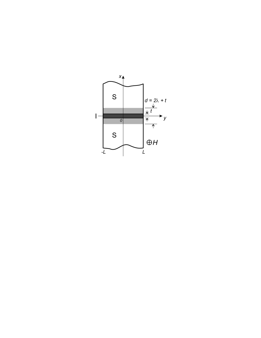
Figure 1: The geometry of the problem: $t$ is the thickness of the barrier; $W=2L$ is the length of the barrier; $\lambda$ is the London penetration depth; $d=2\lambda+t$ is the width of the field-penetration region (shaded). The external magnetic field $H$ is directed into the plane of the figure.

The difficulties of most previous approaches to the problem arose from the incompleteness of a traditional formulationKY72 ; BP82 ; K66 ; OS67 in terms of a static (time-independent) sine-Gordon equation

$$\frac{d^{2}\phi}{dy^{2}}=\frac{1}{\lambda_{J}^{2}}\sin\phi$$ (1)

for the phase difference $\phi=\phi\left(y\right)$ and physical boundary conditions

$$\frac{d\phi}{dy}\left(\pm L\right)=2edH\quad\left(\hbar=c=1\right).$$ (2)

Indeed, equations (1), (2) constitute an ill-posed boundary-value problemCH in the sense that they do not meet the requirement of the uniqueness of the solution. [This is a consequence of nonlinearity of Eq. (1) and of the physical boundary conditions being imposed on $\frac{d\phi}{dy}$ instead of $\phi$.] Thus, although the general solution to (1) was well-known,A70 the constants of integration specifying all physically observable configurations could not be unambiguously determined from boundary conditions (2) alone.

An obvious way to overcome the problem of incompleteness lies in an observation that Eqs. (1), (2) are nothing but stationarity conditions of a relevant Gibbs free-energy functional.K04 ; K05 Therefore, among all solutions to (1) that satisfy (2) at a given $H$, one has to choose those that minimize (at least locally) the Gibbs free-energy functional. By general physical arguments, the stable (in a mathematical sense) solutions should represent an observable thermodynamically stable state (in the case of an absolute minimum), as well as observable thermodynamically metastable states (in the case of local minima). Unfortunately, the issue of exact minimization of the Gibbs free-energy functional did not receive appropriate attention in the previous literature. (However, stability of some particular solutions was analyzed from a somewhat different point of view, e.g., in Refs. Ga84 ; Yu94 ; Se04 .)

The fact that a complete set of stable solutions to (1), (2) can be obtained in a closed analytical form has been first demonstrated in Refs. K04 ; K05 within the framework of minimization of a certain wide class of energy functionals whose particular representative is the Gibbs free-energy functional of a single Josephson junction. Exact analytical solutions of Refs. K04 ; K05 form an infinite set and are labelled by a topological (vortex) number $N_{v}=0,1,2,\ldots$. As is pointed out in Refs. K04 ; K05 , these solutions constitute a new class of particular solutions to the sine-Gordon equation that can be interpreted as nontrivial ”vacuum” (for $N_{v}=0$) and static topological solitons (for $N_{v}=1,2,\ldots$) in a finite spatial interval. Solutions of this type were not considered in the previous literature on the sine-Gordon equation.L80 ; DEGM82 ; KK89

In what follows, we show that the new topological solutions resolve the problem formulated at the beginning of the Introduction. To make the paper self-contained and independent of Refs. K04 ; K05 , we employ a new, more general method of the derivation of topological solutions. In particular, we start with a full set of solutions to (1), (2). In contrast to the approach of Refs. K04 ; K05 , the selection of stable (physical) solutions is made by explicit evaluation of the sign of the second variation of the Gibbs free-energy functional, which allows us to establish general conditions of stability.

In section II, we introduce the Gibbs free-energy functional and show that all its stationary points are either minima or saddle points. In section III, the second variation of the Gibbs free energy is discussed. We show that the sign of the second variation is related to the sign of the lowest eigenvalue of a certain Sturm-Liouville eigenvalue problem. In this way, we establish general conditions of stability. In section IV, a full set of solutions to (1), (2) is obtained and classified with respect to stability. In section V, a full set of stable (physical) solutions to (1), (2) is derived. These solutions comprise a Meissner solution ($N_{v}=0$) and vortex solutions ($N_{v}=1,2,\ldots$). Their major physical and mathematical properties are thoroughly discussed. An exact, closed-form expression for the Gibbs free energy is derived. This expression is analyzed numerically in the cases of a ”large” junction and a ”small” junction. In section VI, unstable (saddle-point) solutions to (1), (2) are classified and discussed. In section VII, we summarize the main results of the paper and make a few concluding remarks. Finally, in appendix A, we analyze stability in two singular cases (the Meissner solution in a semiinfinite interval and the single-soliton solution in an infinite interval).

II Gibbs free-energy functional: Major properties

From now on, we will employ dimensionless units. Thus, the length scale along the $y$ axis is normalized to the Josephson penetration length $\lambda_{J}$. The magnetic field is normalized to the superheating field of the Meissner state in a semi-infinite junctionKY72 $H_{s}=\left(ed\lambda_{J}\right)^{-1}$. The energy scale is normalized to $\frac{d\lambda_{J}H_{s}^{2}}{16}$. (In particular, the flux quantum in our dimensionless units is given by $\Phi_{0}=\pi$.)

In terms of the dimensionless units, a phase-dependent part of the Gibbs free-energy functional per unit length along the $z$ axis takes the formK04 ; K05

$$\Omega_{G}\left[\phi,\frac{d\phi}{dy};H\right]=2H^{2}W+\int\limits_{-L}^{L}dy\left[1-\cos\phi\left(y\right)+\frac{1}{2}\left[\frac{d\phi\left(y\right)}{dy}\right]^{2}\right]-2H\left[\phi\left(L\right)-\phi\left(-L\right)\right].$$ (3)

Note that the last term in Eq. (3) is, physically, proportional to the magnetic (Josephson) flux

$$\Phi_{J}=\frac{1}{2}\left[\phi\left(L\right)-\phi\left(-L\right)\right],$$ (4)

with

$$h\left(y\right)=\frac{1}{2}\frac{d\phi}{dy}$$ (5)

being the corresponding local magnetic field (equilibrium or not).

The stationarity condition of the Gibbs free-energy functional (3),

$$\delta\Omega_{G}\left[\phi,\frac{d\phi}{dy};H\right]=0,$$ (6)

reduces to the static sine-Gordon equation for the phase difference

$$\frac{d^{2}\phi}{dy^{2}}=\sin\phi$$ (7)

and boundary conditions

$$\frac{d\phi}{dy}\left(\pm L\right)=2H\geq 0.$$ (8)

[Compare with Eqs. (1) and (2), respectively, where dimensional units are employed.]

The main property of the functional (3) follows from the fact that it belongs to the class of regular functionals, i.e., satisfies a necessary condition of the minimum;A62 hence, all stationary points of (3) are either minima of saddle points. [Unfortunately, the statement of Ref. Yu94 that all stationary points of (3) ”are minima” is incorrect.]

As already mentioned in the Introduction, boundary conditions (8) do not ensure the uniqueness of the solution to Eq. (7). Moreover, solutions to (7), (8), as stationary points of the Gibbs free-energy functional (3), can correspond to either minima or saddle points of this functional. Taking into account that only stable phase configurations, corresponding to minima of (3), are physically observable, the problem one has to solve can be formulated as follows: Find all solutions to (7), (8) that minimize (at least locally) (3) at given $H\geq 0$. To resolve this problem, we have to turn to sufficient conditions of the minimum,A62 which requires an analysis of the second variation of (3).

III Second variation of the Gibbs free-energy functional and a related Sturm-Liouville eigenvalue problem

Let $\phi=\bar{\phi}\left(y\right)$ be a particular solution to (7), (8) [i.e., a certain stationary point of (3)]. The increment of the Gibbs free-energy functional (3) in the vicinity of this solution, induced by variations $\bar{\phi}\left(y\right)\rightarrow\bar{\phi}\left(y\right)+\delta\phi\left(y\right)$, where $\delta\phi$ has a continuous derivative that obeys boundary conditions

$$\frac{d\delta\phi}{dy}\left(-L\right)=\frac{d\delta\phi}{dy}\left(L\right)=0,$$ (9)

can be expanded in an infinite series:A62

$$\Delta\Omega_{G}\left[\delta\phi,\frac{d\delta\phi}{dy};H\right]_{\phi=\bar{\phi}}=\frac{1}{2!}\delta^{2}\Omega_{G}\left[\delta\phi,\frac{d\delta\phi}{dy}\right]_{\phi_{n}=\bar{\phi}_{n}}+\sum_{k\geq 3}\frac{1}{k!}\delta^{k}\Omega_{G}\left[\delta\phi\right]_{\phi=\bar{\phi}}.$$ (10)

Here,

$$\delta^{2}\Omega_{G}\left[\delta\phi,\frac{d\delta\phi}{dy}\right]_{\phi=\bar{\phi}}=\int\limits_{-L}^{L}dy\left[\cos\bar{\phi}\left(y\right)\left[\delta\phi\left(y\right)\right]^{2}+\left[\frac{d\delta\phi}{dy}\left(y\right)\right]^{2}\right],$$ (11)

and

$$\delta^{k}\Omega_{G}\left[\delta\phi\right]_{\phi=\bar{\phi}}=-\int\limits_{-L}^{L}dy\cos\left[\bar{\phi}\left(y\right)+\frac{k\pi}{2}\right]\left[\delta\phi\left(y\right)\right]^{k},\quad k\geq 3.$$ (12)

The sign of the second variation (11) in the expansion (10) determines a type of the tested solution $\phi=\bar{\phi}\left(y\right)$. Three different cases are possible: (i) the case

$$\delta^{2}\Omega_{G}\left[\delta\phi,\frac{d\delta\phi}{dy}\right]_{\phi=\bar{\phi}}>0$$ (13)

corresponds to a minimum of (3), (i.e., the solution is inside a stability region); (ii) the case

$$\delta^{2}\Omega_{G}\left[\delta\phi,\frac{d\delta\phi}{dy}\right]_{\phi=\bar{\phi}}\geq 0,$$ (14)

corresponds to a boundary of the stability region (a bifurcation point),Th82 when the solution can loose stability with respect to a certain variation; (iii) finally, if $\delta^{2}\Omega_{G}\left[\delta\phi,\frac{d\delta\phi}{dy}\right]_{\phi=\bar{\phi}}$ has no definite sign, the solution corresponds to a saddle point of (3), which means absolute instability. Therefore, in what follows, we concentrate ourselves on the evaluation of $\delta^{2}\Omega_{G}$.

As is shown in variational theory of eigenvalues,LL50 the functional $\delta^{2}\Omega_{G}$ satisfies the following general relation:r1

$$\delta^{2}\Omega_{G}\left[\delta\phi,\frac{d\delta\phi}{dy}\right]_{\phi=\bar{\phi}}\geq\mu_{0}\int\limits_{-L}^{L}dy\left[\delta\phi\left(y\right)\right]^{2},$$ (15)

where $\mu_{0}$ is the lowest eigenvalue of the Sturm-Liouville eigenvalue problem

$$-\frac{d^{2}\psi}{dy^{2}}+\cos\vec{\phi}\left(y\right)\psi=\mu\psi,\quad y\in\left[-L,L\right],$$ (16)

$$\frac{d\psi}{dy}\left(-L\right)=\frac{d\psi}{dy}\left(L\right)=0.$$ (17)

Equality on the right-hand side of relation (15) is achieved, when $\delta\phi$ coincides (up to a factor) with the eigenfunction corresponding to $\mu_{0}$: i.e., $\delta\phi\equiv const\,\psi_{0}$. As is clear from relation (15), the three different types (i)-(iii) of the behavior of $\delta^{2}\Omega_{G}$ correspond, respectively to: (i) $\mu_{0}>0$; (ii) $\mu_{0}=0$; (iii) $\mu_{0}<0$.

The properties of the self-adjoint operator, specified by the left-hand side of Eq. (16) and boundary conditions (17), are well-known.LS70 In particular, its spectrum $\mu_{n}$ ($n=0,1,2,\ldots$) is discrete, real, infinite and bounded from below:

$$\mu_{0}<\mu_{1}<\mu_{2}<\ldots$$ (18)

(Note that in our case $\left|\mu_{0}\right|\leq 1$.) The corresponding eigenfunctions $\psi_{n}$ ($n=0,1,2,\ldots$) are real, mutually orthogonal and can be normalized:

$$\int\limits_{-L}^{L}dy\psi_{n}\left(y\right)\psi_{m}\left(y\right)=0,\quad n\neq m;\quad 0<\int\limits_{-L}^{L}dy\left[\psi_{n}\left(y\right)\right]^{2}<\infty.$$ (19)

The eigenvalue number $n$ determines the number of nodes of the eigenfunction $\psi_{n}$ in the interval $\left[-L,L\right]$ . Thus, the eigenfunction $\psi_{0}$ can be considered strictly positive:

$$\psi_{0}=\psi_{0}\left(y\right)>0,\quad y\in\left[-L,L\right].$$ (20)

Significantly, the set of eigenfunctions $\left\{\psi_{n}\right\}_{n=0}^{\infty}$ is complete in the sense that any function $f\left(y\right)$ that possesses continuous derivatives up to the second order and obeys boundary conditions $f\left(\pm L\right)=0$ can be expanded in terms of $\psi_{n}.$

Upon substitution of a solution of the boundary-value problem (7), (8) into (16), this equation can be transformed into the well-knownWW27 Lamé equation. Therefore, the boundary-value problem for $\mu=\mu_{0}$ can, in principle, be solved analytically. However, since we need to know only the sign of $\mu_{0}$, we will derive below a set of exact relations that will allow us to determine the sign of $\mu_{0}$ without explicit evaluation of $\mu_{0}$.

First, we notice that the function

$$\chi\equiv\frac{d\phi}{dy},$$ (21)

where $\phi=\phi\left(y\right)$ is a particular solution to (7), (8) (in what follows, we drop the bar over $\vec{\phi}$), satisfies the equation

$$-\frac{d^{2}\chi}{dy^{2}}+\cos\phi\left(y\right)\chi=0.$$ (22)

Combining (21), (22) and (16) (with $\mu=\mu_{0}$, $\psi=\psi_{0}$), using boundary conditions (17), we obtain the sought relations

$$\mu_{0}=\frac{\psi_{0}\left(L\right)\frac{d^{2}\phi}{dy^{2}}\left(L\right)-\psi_{0}\left(-L\right)\frac{d^{2}\phi}{dy^{2}}\left(-L\right)}{\int\limits_{-L}^{L}dy\psi_{0}\left(y\right)\frac{d\phi}{dy}\left(y\right)}=\frac{\psi_{0}\left(L\right)\sin\phi\left(L\right)-\psi_{0}\left(-L\right)\sin\phi\left(-L\right)}{\int\limits_{-L}^{L}dy\psi_{0}\left(y\right)\frac{d\phi}{dy}\left(y\right)}.$$ (23)

[For definiteness, we choose the sign of $\psi_{0}$ according to (20).] In addition, we note that, if $\psi_{0}$ is known explicitly, $\mu_{0}$ can be found from the relation

$$\mu_{0}=\frac{\int\limits_{-L}^{L}dy\psi_{0}\left(y\right)\cos\phi\left(y\right)}{\int\limits_{-L}^{L}dy\psi_{0}\left(y\right)}.$$ (24)

IV Complete set of solutions and their classification with respect to stability

We begin with the first integral of Eq. (7):

$$\frac{1}{2}\left[\frac{d\phi}{dy}\right]^{2}+\cos\phi=C,\quad-1\leq C<\infty,$$ (25)

where $C\,$ is the constant of integration. Using (25), it is straightforward to derive the general solution to (7).A70 We write down this solution in the following explicit form:

(I) $-1\leq C\leq 1$:

$$\phi_{\pm}\left(y\right)=\pi\left(2n+1\right)\pm 2\arcsin\left[k\,sn\left(y-y_{0},k\right)\right],\quad n=0,\pm 1,\ldots,$$ (26)

$$-K\left(k\right)\leq y_{0}<K\left(k\right),\quad k\equiv\frac{1+C}{2},\quad 0\leq k\leq 1;$$

(II) $1\leq C<\infty$:

$$\phi_{\pm}\left(y\right)=\pi\left(2n+1\right)\pm 2\,am\left(\frac{y-y_{0}}{k},k\right),\quad n=0,\pm 1,\ldots,$$ (27)

$$-kK\left(k\right)\leq y_{0}<kK\left(k\right),\quad k\equiv\frac{2}{1+C},\quad 0<k\leq 1.$$

Here, the functions $am\,u$ and $sn\,u$ are the Jacobi elliptic amplitude and the elliptic sine, respectively; $K\left(k\right)$ is the complete elliptic integral of the first kind.AS65 The choice of sign (i.e., $\phi_{+}$ or $\phi_{-}$) and allowed values of the constants of integration $y_{0}$, $k$ in (26), (27) should be determined from the requirement of compatibility with boundary conditions (8) that we rewrite in a somewhat generalized form:

$$\frac{d\phi}{dy}\left(-L\right)=const\geq 0,\quad\frac{d\phi}{dy}\left(L\right)=const\geq 0;$$ (28)

$$\frac{d\phi}{dy}\left(-L\right)=\frac{d\phi}{dy}\left(L\right).$$ (29)

IV.1 Solutions of type I

Consider solutions of type I [Eqs. (26)]. First, we note that, for this type of solutions,

$$\left|\phi\left(L\right)-\phi\left(-L\right)\right|<2\pi$$ (30)

for any $0<L<\infty$. Taking into account that

$$\frac{d\phi_{\pm}}{dy}=\pm 2k\,cn\,\left(y-y_{0},k\right),$$ (31)

where $\,cn\,u$ is the elliptic cosine, from  (28) we find that the appropriate solution is $\phi=\phi_{+}$. If $L\leq\frac{\pi}{2}$, the constant of integration $k\in\left[0,1\right]$. In contrast, for $L>\frac{\pi}{2}$, the allowed values for $k$ are $k=0$ and $k\in\left[k_{m},1\right]$, where $k_{m}$ is determined from the condition

$$K\left(k_{m}\right)=L.$$ (32)

Condition (29) yields an equation for $y_{0}$,

$$sn\,\left(L,k\right)dn\,\left(L,k\right)sn\,\left(y_{0},k\right)dn\,\left(y_{0},k\right)=0$$

(where $dn\,u=\frac{d}{du}am\,u$), whose unique solution is $y_{0}=0$. Thus, solutions of type I, compatible with boundary conditions (8), have the form

$$\phi\left(y\right)=\pi\left(2n+1\right)+2\arcsin\left[k\,sn\left(y,k\right)\right],\quad n=0,\pm 1,\ldots,$$ (33)

where $k\in\left[0,1\right]$ for $L\leq\frac{\pi}{2}$, and $k=0$, $k\in\left[k_{m},1\right]$ for $L>\frac{\pi}{2}$.

An analysis of stability of solutions (33) is straightforward. Thus, for $k=0$ we have

$$\phi\left(y\right)=\pi\left(2n+1\right),\quad n=0,\pm 1,\ldots.$$ (34)

The exact eigenfunction in (24) is $\psi_{0}=const>0$, which immediately yields $\mu_{0}=-1$. For $k\neq 0$, the denominator in (23) is positive, whereas

$$\frac{d^{2}\phi}{dy^{2}}\left(L\right)\equiv-sn\,\left(L,k\right)dn\,\left(L,k\right)<0,\quad\frac{d^{2}\phi}{dy^{2}}\left(-L\right)\equiv sn\,\left(L,k\right)dn\,\left(L,k\right)>0.$$

Therefore, $\mu_{0}<0$. In other words, solutions (33) correspond to saddle points of (3) and, hence, are unstable and physically unobservable.

IV.2 Solutions of type II

Consider solutions of type II [Eqs. (27)]. In contrast to the solutions of type I [see (30)], now

$$\left|\phi\left(L\right)-\phi\left(-L\right)\right|<\infty$$ (35)

for any $0<L<\infty$. Using the derivative

$$\frac{d\phi_{\pm}}{dy}=\pm\frac{2}{k}\,dn\,\left(\frac{y-y_{0}}{k},k\right),$$ (36)

from  (28) we conclude that the appropriate solution is $\phi=\phi_{+}$, with $k\in\left(0,1\right]$. Condition (29) yields an equation for $y_{0}$,

$$sn\,\left(\frac{L}{k},k\right)cn\,\left(\frac{L}{k},k\right)sn\,\left(\frac{y_{0}}{k},k\right)cn\,\left(\frac{y_{0}}{k},k\right)=0.$$ (37)

If $\frac{L}{k}\neq pK\left(k\right)$ ($p=1,2,\ldots$) in (37), this equation has two different solutions:

$$y_{0}=-kK\left(k\right),\quad y_{0}=0.$$ (38)

Correspondingly, solutions (27), compatible with boundary conditions (8), split into two distinct sets:

$$\phi_{e}\left(y\right)=\pi\left(2n+1\right)+2\,am\left(\frac{y}{k}+K\left(k\right),k\right),\quad n=0,\pm 1,\ldots,$$ (39)

and

$$\phi_{o}\left(y\right)=\pi\left(2n+1\right)+2\,am\left(\frac{y}{k},k\right),\quad n=0,\pm 1,\ldots.$$ (40)

The meaning of the subscripts $e$ (even) and $o$ (odd) should be clear from the following: for solutions (39), we have $\phi_{e}\left(0\right)=2\pi\left(n+1\right)$ ($n=0,\pm 1,\ldots$); in contrast, for solutions (40), $\phi_{o}\left(0\right)=\pi\left(2n+1\right)$ ($n=0,\pm 1,\ldots$). Using Eq. (7) and its derivative,

$$\frac{d^{3}\phi}{dy^{3}}=\cos\phi\frac{d\phi}{dy},$$ (41)

we find that the ”local magnetic field” (5) at $y=0$ has a minimum for $\phi_{e}$ and a maximum for $\phi_{o}$.

It is interesting to note that the two sets of solutions (39), (40) are related by the Bäcklund transformations

$$\frac{1}{2}\frac{d}{dy}\left[\phi_{o}\pm\phi_{e}\right]=\frac{1\pm\sqrt{1-k^{2}}}{k}\sin\frac{\phi_{o}\mp\phi_{e}}{2},$$

which, in the general case of a time-dependent sine-Gordon equation, is a hallmark of complete integrability.L80 ; DEGM82 ; KK89 By virtue of the symmetry relations

$$\phi_{e}\left(-y\right)=-\phi_{e}\left(y\right)+4\pi\left(n+1\right),$$

$$\phi_{o}\left(-y\right)=-\phi_{o}\left(y\right)+2\pi\left(2n+1\right),$$

the eigenfunction $\psi_{0}$ in (16), (17) is necessarily symmetric with respect to reflection: $\psi_{0}\left(-y\right)=\psi_{0}\left(y\right)$. As a result, for $\delta\phi\equiv const\,\psi_{0}$, all the odd terms $\delta^{2m+1}\Omega_{G}$ ($m=1,2,\ldots$) in expansion (10) vanish by symmetry.

Stability regions for solutions (39) and (40) can be established as follows. First, we note that the roots of the equations

$$pkK\left(k\right)=L,\quad p=1,2,\ldots,$$ (42)

$k=k_{p}\in\left(0,1\right]$, form an infinite decreasing sequence of bifurcation points:

$$1>k_{1}>k_{2}>\ldots$$ (43)

Indeed, the second derivatives of $\phi_{e}$ and $\phi_{o}$, respectively, read:

$$\frac{d^{2}\phi_{e}}{dy^{2}}\left(y\right)=2\sqrt{1-k^{2}}\frac{sn\,\left(\frac{y}{k},k\right)cn\,\left(\frac{y}{k},k\right)}{dn^{2}\,\left(\frac{y}{k},k\right)},\quad\frac{d^{2}\phi_{o}}{dy^{2}}\left(y\right)=-2sn\,\left(\frac{y}{k},k\right)cn\,\left(\frac{y}{k},k\right).$$ (44)

Using (44), we find

$$\frac{d^{2}\phi_{e,o}}{dy^{2}}\left(\pm L\right)=0$$ (45)

for $k=k_{p}$ ($p=1,2,\ldots$). Substituting $\phi=\phi_{e,o}$ with $k=k_{p}$ ($p=1,2,\ldots$) into (23), using (45) and the fact that the denominator in (23) is strictly positive, we find $\mu_{0}=0$ both for $\phi=\phi_{e}$ and $\phi=\phi_{o}$. [As a matter of fact, the derivatives $\frac{d\phi_{e,o}}{dy}$, for $k=k_{p}$ ($p=1,2,\ldots$), coincide (up to a normalization factor) with the eigenfunctions $\psi_{0\,e,o}$ corresponding to the eigenvalues $\mu_{0\,e,o}=0$.]

The bifurcation points $k=k_{p}$ ($p=1,2,\ldots$) subdivide the interval $I\equiv\left(0,1\right]$ into an infinite set of semi-open intervals:

$$I=\cup_{p=0}^{\infty}I_{p},$$ (46)

where

$$I_{0}=\left(k_{1},1\right];\quad I_{p}=\left(k_{p+1},k_{p}\right],\quad p=1,2,\ldots.$$ (47)

The index of these intervals $p=0,1,2,\ldots$ can be expressed as

$$p=\left[\frac{\phi_{e,o}\left(L\right)-\phi_{e,o}\left(-L\right)}{2\pi}\right],$$ (48)

where $\left[\ldots\right]$ stands for the integer part of the argument. As can be easily verified using (23) and (44), $\mu_{0\,e}>0$ and $\mu_{0\,o}<0$ for $k\in I_{0}$; $\mu_{0\,e}\geq 0$ and $\mu_{0\,o}\leq 0$ for $k\in I_{2m}$ ($m=1,2,\ldots$); $\mu_{0\,e}\leq 0$ and $\mu_{0\,o}\geq 0$ for $k\in I_{2m+1}$ ($m=0,1,2,\ldots$). [We again emphasize that the equalities $\mu_{0\,e,o}=0$ are realized only at the bifurcation points $k=k_{p}$ ($p=1,2,\ldots$).] On these grounds, we conclude that stability regions for the solutions $\phi=\phi_{e}$ are given by the intervals $I_{2m}$ ($m=0,1,2,\ldots$), whereas stability regions for the solutions $\phi=\phi_{o}$ are given by the intervals $I_{2m+1}$ ($m=0,1,2,\ldots$).

It is instructive to illustrate the above general results by explicit evaluation of $\mu_{0}=\mu_{0}\left(k\right)$ for $k\ll 1$. In this limit, the lowest eigenvalue $\mu_{0}$ can be expanded in a power series of $k$:

$$\mu_{0}=\sum_{n\geq 1}\mu_{0}^{\left(n\right)}\left(k\right),$$

where $\mu_{0}^{\left(n\right)}\left(k\right)$ is of order $k^{n}$ ($n=1,2,\ldots$). Here, we restrict ourselves to the evaluation of $\mu_{0}^{\left(1\right)}\left(k\right)$: i.e., $\mu_{0}\approx\mu_{0}^{\left(1\right)}\left(k\right)$. In view of the asymptotic expansions

$$\phi_{e}\left(y\right)\approx 2\pi\left(n+1\right)+\frac{2y}{k}-\frac{ky}{2}-\frac{k^{2}}{4}\sin\frac{2y}{k},\quad n=0,\pm 1,\ldots,$$ (49)

$$\phi_{o}\left(y\right)\approx\pi\left(2n+1\right)+\frac{2y}{k}-\frac{ky}{2}+\frac{k^{2}}{4}\sin\frac{2y}{k},\quad n=0,\pm 1,\ldots.,$$ (50)

it is sufficient to take a zeroth-order approximation to $\psi_{0}$: $\psi_{0}\approx\psi_{0}^{\left(0\right)}$. In zeroth order in $k$, equations (16), (17) for $\psi_{0}$ become

$$\frac{d^{2}\psi_{0}^{\left(0\right)}}{dy^{2}}=0,\quad\frac{d\psi_{0}^{\left(0\right)}}{dy}\left(-L\right)=\frac{d\psi_{0}^{\left(0\right)}}{dy}\left(L\right)=0,$$

whose solution is

$$\psi_{0\,e,o}^{\left(0\right)}=const.$$ (51)

Upon substitution of (49)-(51) into (24), we obtain

$$\mu_{0\,e}^{\left(1\right)}=k\sin\frac{W}{k},\quad\mu_{0\,o}^{\left(1\right)}=-k\sin\frac{W}{k}.$$ (52)

Expressions (52) immediately yield bifurcation points for $k\ll 1$:

$$k_{p}=\frac{W}{\pi p},\quad p=1,2,\ldots,$$ (53)

in full agreement with (42).

Summarizing, in this section we have derived a complete set of the solutions to (7) (both stable and unstable), compatible with boundary conditions (8). The only stable solutions [i.e., corresponding to the minima of (3)] are those given by Eq. (39) and Eq. (40), where $k\in I_{2m}$ ($m=0,1,2,\ldots$) and $k\in I_{2m+1}$ ($m=0,1,2,\ldots$), respectively. In the next two sections both the stable and unstable solutions will be analyzed in more detail.

V Stable Meissner and vortex (soliton) solutions

It is convenient to introduce a unified classification of the stable solutions, directly related to their physical interpretation. To this end, we introduce a new integer, the vortex (or topological) number $N_{v}=0,1,\ldots$, by means of the definition

$$N_{v}\equiv p=\left[\frac{\phi\left(L\right)-\phi\left(-L\right)}{2\pi}\right]=\left[\frac{1}{2\pi}\int\limits_{-L}^{L}dy\frac{d\phi}{dy}\right]$$ (54)

[compare Eq. (48)], and fix the so far arbitrary integer $n=0,\pm 1,\pm 2,\ldots$ in Eqs. (39) and (40) by the condition

$$\phi\left(0\right)=\pi N_{v}.$$ (55)

[Here, $\phi=\phi_{e}$ for $N_{v}=2m$ ($m=0,1,2,\ldots$), and $\phi=\phi_{o}$ for $N_{v}=2m+1$ ($m=0,1,2,\ldots$).] Finally, using boundary conditions (8) for the determination of $k$, we arrive at the desired form for the stable solutions:K04 ; K05

$$\phi_{e}(y)=\pi\left(N_{v}-1\right)+2\,am\,\left(\frac{y}{k}+K\left(k\right),k\right),\quad k=k\left(H\right):$$ (56)

$$dn\,\left(\frac{L}{k},k\right)=\frac{\sqrt{1-k^{2}}}{kH},\qquad N_{v}=2m\quad\left(m=0,1,\ldots\right);$$ (57)

$$\phi_{o}(y)=\pi N_{v}+2\,am\,\left(\frac{y}{k},k\right),\quad k=k\left(H\right):$$ (58)

$$dn\,\left(\frac{L}{k},k\right)=kH,\qquad N_{v}=2m+1\quad\left(m=0,1,\ldots\right),$$ (59)

where $N_{v}=0$ corresponds to the vortex-free Meissner (”vacuum”) solution, and $N_{v}=1,2\ldots$ correspond to vortex (soliton) solutions. The stability regions in terms of the field $H$ take the form

$$0\leq H<H_{0},\quad N_{v}=0,$$ (60)

$$\sqrt{H_{N_{v}-1}^{2}-1}\leq H<H_{N_{v}},\quad N_{v}=1,2,\ldots,$$ (61)

with $H_{N_{v}}$ implicitly determined by

$$\left(N_{v}+1\right)K\left(\frac{1}{H_{N_{v}}}\right)=H_{N_{v}}L.$$ (62)

According to the results of section IV, we have $\delta^{2}\Omega_{G}>0$ within the whole semi-open interval (60). Analogously, $\delta^{2}\Omega_{G}>0$ inside the semi-open intervals (61), whereas $\delta^{2}\Omega_{G}\geq 0$ at their boundaries. [Note that the upper bounds of the stability regions (60), (61) are also determined by the condition $\delta^{2}\Omega_{G}\geq 0$.]

Solutions (56)-(62) satisfy the symmetry relations

$$\phi\left(-y\right)=-\phi\left(y\right)+2\pi N_{v}$$ (63)

and obey the boundary conditions

$$-\pi<\phi\left(-L\right)\leq 0,\quad 2\pi N_{v}\leq\phi\left(L\right)<2\pi\left(N_{v}+\frac{1}{2}\right),$$ (64)

which ensures the fulfillment of the stability conditions

$$\frac{d^{2}\phi}{dy^{2}}\left(-L\right)\leq 0,\quad\frac{d^{2}\phi}{dy^{2}}\left(L\right)\geq 0.$$ (65)

As to major properties of the stable solutions, we want to emphasize the following.

The stable solutions form an infinite set and their existence regions (60), (61) overlap (at least for two neighboring states). This fact not only ensures that the stable solutions cover the whole field range $0\leq H<\infty$, but also proves that hysteresis is an intrinsic property of any Josephson junction, irrespectively of the value of $W<\infty$. However, overlapping is stronger for larger values of $W$ and at $1\ll W<\infty$ may involve several neighboring states. On the other hand, overlapping decreases with an increase of $H$.

Soliton (vortex) solutions with $N_{v}=1,2,\ldots$ exist for arbitrary small $W<\infty$, provided the field $H>0$ is sufficiently high. We also note that the single-soliton ($N_{v}=1$) solution appears at a finite (for any $W<\infty$) field $H=\sqrt{H_{0}^{2}-1}>0$ , which should be contrasted with the case of the infinite interval $\left(-\infty,+\infty\right)$: see Eq. (68) below.

Solutions with $N_{v}=1,2,\ldots$are pure solitons only at $H=\sqrt{H_{N_{v}-1}^{2}-1}$, when $\phi\left(-L\right)=0$, $\phi\left(L\right)=2\pi N_{v}$ and $\delta^{2}\Omega_{G}\geq 0$. In the rest of the stability regions (61), when $\delta^{2}\Omega_{G}>0$, we have solitons ”dressed” by the Meissner field. As a matter of fact, solitons (vortices) are confined to the spatial interval $\left[-l,l\right]$, where $l$ is determined from the conditions $\phi\left(-l\right)=0$, $\phi\left(l\right)=2\pi N_{v}$. In contrast, the intervals $\left[-L,-l\right)$ and $\left(l,L\right]$ are ”reserved” for the Meissner field. Nevertheless, although Josephson vortices always exist against a background of the Meissner field, solutions (56)-(62) with $N_{v}=1,2,\ldots$ by no means can be thought of as a mere superposition of the Meissner and the vortex fields, because the principle of superposition does not hold for the non-linear equation (13).

A solution with $N_{v}=0,1,2,\ldots$ solitons cannot be continuously transformed into the solution with $N_{v}+1$ solitons and vice versa. Therefore, any transitions between configurations with different vortex numbers $N_{v}$ are necessarily thermodynamic first-order phase transitions.

Some examples of the stable solutions (for $N_{v}=0,1,2$), obtained by numerical evaluation of (56)-(62), are presented in Fig. 2. In several particular cases, known from the previous literature, solutions (56)-(62) can be expressed in terms of elementary functions. For example, at $H=0$ and arbitrary $L<\infty$, there exists only the trivial Meissner ($N_{v}=0$) solution $\phi_{0}\left(y\right)\equiv 0$, $y\in\left[-L,L\right]$. In the low-field limit $0\leq H\ll 1$, the Meissner solution [equation (56) with $N_{v}=0$] reads:

$$\phi_{0}\left(y\right)\approx\frac{2H}{\cosh L}\sinh y,\quad h\left(y\right)\approx\frac{H}{\cosh L}\cosh y.$$

Figure 2: Stable solutions for $L=3.0$. (a) The Meissner solution ($N_{v}=0$): curves 1 and 2 correspond to the cases $0<H<H_{0}$ and $H=H_{0}$, respectively. (b) The single-vortex solution ($N_{v}=1$): curves 1-3 correspond to the cases $H=\sqrt{H_{0}^{2}-1}$, $\sqrt{H_{0}^{2}-1}<H<H_{1}$ and $H=H_{1}$, respectively; the vortex is confined to the spatial intervals denoted by vertical arrows. (c) The two-vortex solution ($N_{v}=2$): curves 1-3 correspond to the cases $H=\sqrt{H_{1}^{2}-1}$, $\sqrt{H_{1}^{2}-1}<H<H_{2}$ and $H=H_{2}$, respectively; the vortices are confined to the spatial intervals denoted by vertical arrows.

By changing the variable $y\rightarrow y-L$ and proceeding to the limit $L\rightarrow\infty$ in equations (56), (57) with $N_{v}=0$, we obtain the exact Meissner solution in a semiinfinite interval:KY72

$$\phi_{0\,\infty}(y)=-4\arctan\frac{H\exp\left(-y\right)}{1+\sqrt{1-H^{2}}},\quad y\in[0,+\infty).$$ (66)

Equation (66) immediately yields the upper bound of the existence of the Meissner state (or the superheating field of the Meissner state) in the semiinfinite junction: $H_{0}\equiv H_{s}=1$. The local magnetic field induced by (66),

$$h\left(y\right)=\frac{H\left(1+\sqrt{1-H^{2}}\right)}{\left(1+\sqrt{1-H^{2}}\right)\exp y-H^{2}\sinh y},\quad y\in[0,+\infty),$$ (67)

vanishes at $y=+\infty$, as it should.

By proceeding to the limit $\pm$$L\rightarrow\pm\infty$, $H\rightarrow 0$, we find two different solutions: namely, the trivial Meissner ($N_{v}=0$) solution $\phi_{0}\left(y\right)\equiv 0$, $y\in\left(-\infty,+\infty\right)$, and the well-known single-soliton ($N_{v}=1$) solution in an infinite intervalL80 ; DEGM82 ; KK89

$$\phi_{1\,\infty}(y)=4\arctan\exp y,\quad y\in(-\infty,+\infty).$$ (68)

The local magnetic field induced by (68),

$$h\left(y\right)=\cosh{}^{-1}y,\quad y\in(-\infty,+\infty),$$ (69)

vanishes at $y=\pm\infty$. Note that, from a point of view of the analysis of stability, solutions (66), (68) constitute singular cases: see appendix A.

Of particular interest is the limit $H\gg\max\left\{1,W\right\}$, which, physically, corresponds to negligibly small screening by Josephson currents. In this limit, the overlapping of states with different $N_{v}$ practically vanishes, and equations (57)-(59) becomeK99

$$\phi_{e,o}(y)\approx\pi N_{v}+2Hy-\frac{\left(-1\right)^{N_{v}}}{4H^{2}}\left[\sin\left(2Hy\right)-2Hy\cos\left(HW\right)\right],$$ (70)

where $N_{v}=\left[\frac{HW}{\pi}\right]$, according to (54). The distribution of the local magnetic field induced by (70) is

$$h\left(y\right)\approx H-\frac{\left(-1\right)^{N_{v}}}{4H}\left[\cos\left(2Hy\right)-\cos\left(HW\right)\right].$$ (71)

Equations (70), (71) explicitly demonstrate the existence of solitons (or Josephson vortices) in the case $W\ll 1$.

Upon substitution of (56), (57) into (3), we obtain exact, closed-form analytical expressions for the Gibbs free energy. It is convenient to write down these expressions in terms of the average energy density $\omega\left(H,k\right)\equiv\frac{\Omega_{G}\left(H,k\right)}{W}$:

$$\omega\left(H,k\right)=\omega_{e}\left(H,k\right)\delta_{N_{v},2m}+\omega_{o}\left(H,k\right)\delta_{N_{v},2m+1}\quad\left(m=0,1,\ldots\right),$$ (72)

$$\omega_{e}\left(H,k\right)=2H^{2}+\frac{8}{W}\left[\frac{1}{k}E\left(\frac{W}{2k}+K\left(k\right),k\right)-\frac{1}{k}E\left(k\right)\right.\left.-\frac{\left(1-k^{2}\right)W}{4k^{2}}\right]$$

$$-\frac{8H}{W}\left[am\,\left(\frac{W}{2k}+K\left(k\right),k\right)-\frac{\pi}{2}\right],\quad k=k\left(H\right);$$

$$\omega_{o}\left(H,k\right)=2H^{2}+\frac{8}{W}\left[\frac{1}{k}E\left(\frac{W}{2k},k\right)-\frac{\left(1-k^{2}\right)W}{4k^{2}}\right]$$

$$-\frac{8H}{W}am\,\left(\frac{W}{2k},k\right),\quad k=k\left(H\right),$$ (73)

where $\delta_{N_{v},2m}$ and $\delta_{N_{v},2m+1}$ are the Kronecker indices; $E\left(u,k\right)$ and $E\left(k\right)$ are, respectively, the incomplete and complete elliptic integrals of the second kind.AS65 Note that in the limit $H\gg\max\left\{1,W\right\}$ [i.e., in the domain of validity of (70)], equations (72), (V) reduce to

$$\omega\left(H\right)\approx 1-\frac{\left|\sin\left(HW\right)\right|}{HW}+\frac{1}{8H^{2}}\left[\cos{}^{2}\left(HW\right)+\frac{1}{2}\right].$$ (74)

In Figs. 3(a) and 3(b), we present $\omega\left(H\right)$, obtained by numerical evaluation of (72), (V), for the cases of a ”large” ($L=3$) junction and a ”small” ($L=0.3$) junction, respectively. Figure 3(a) exhibits strong overlapping of neighboring stable configurations, whereas in Fig. 3(b) overlapping is practically invisible. The envelope of the energy curves for $N_{v}=0,1,\ldots,6$ corresponds to the absolute minimum of the Gibbs free energy at a given $H$ (a thermodynamically stable configuration). Parts of the energy curves that lie above the envelope in Fig. 3(a) correspond to local minima of the Gibbs free energy (thermodynamically metastable configurations). For better orientation in the physical situation, we have specified the upper bound of the existence of the Meissner state ($H=H_{0}$) and the first thermodynamic critical fieldJ65 ; KY72 ; BP82 ($H=H_{c1}$). (The latter field is determined by the requirement that the Gibbs free energies of the states $N_{v}=0$ and $N_{v}=1$ be equal to each other.) Both the fields, $H_{0}$ and $H_{c1}$, strongly depend on the length $W$: they increase (although at different rates) with a decrease of $W$. For example, for $1\ll W<\infty$, they are approximately given by $H_{0}\approx H_{s}=1$ and $H_{c1}\approx\frac{2}{\pi}$, whereas for $W\ll 1$ they practically coincide: $H_{c1}\approx H_{0}\approx\frac{\pi}{W}$ [see Fig. 3(b)]. Note that by decreasing the external field below $H=H_{c1}$, one can still observe the single-vortex state down to the field $H=\sqrt{H_{0}^{2}-1}<H_{c1}$ [the abscissa of the left end of the energy curve for $N_{v}=1$ in Fig. 3(a)].

Figure 3: The average Gibbs free-energy density $\omega\left(H\right)\equiv\frac{\Omega_{G}\left(H\right)}{W}$ for the cases of a ”large” ($L=3.0$) junction (a) and a ”small” ($L=0.3$) junction (b). Energy curves are shown for $N_{v}=0,1,\ldots,6$. The upper bound of the existence of the Meissner state ($H_{0}$) and the first thermodynamic critical field ($H_{c1}$) are also shown.

VI Unstable (saddle-point) solutions

There are three different types of unstable (saddle-point) solutions to (7), (8). Unstable solutions of the first and the second types obey symmetry relations

$$\phi\left(-y\right)=-\phi\left(y\right)+2\pi Z,$$ (75)

where $Z$ is an integer. In contrast to the stable solutions of section V, this integer cannot be made to satisfy relation

$$Z=\left[\frac{\phi\left(L\right)-\phi\left(-L\right)}{2\pi}\right]$$

by any transformation $\phi\rightarrow\phi+2\pi n$ ($n=0,\pm 1,\ldots$) and, thus, has no meaning of a topological number. In view of (75), the eigenfunction $\psi_{0}$ in (16), (17) is symmetric with respect to reflection: $\psi_{0}\left(-y\right)=\psi_{0}\left(y\right)$. However, in contrast to the stable solutions (56)-(59), the first two types of unstable solutions are characterized by the property

$$\frac{d^{2}\phi}{dy^{2}}\left(L\right)<0,\quad\frac{d^{2}\phi}{dy^{2}}\left(-L\right)>0,$$ (76)

which results in $\mu_{0}<0$ [see (23)].

The first type of unstable solutions is represented by the set (33). Without loss of generality, it is sufficient to consider the case of $n=0$:

$$\phi\left(y\right)=\pi+2\arcsin\left[k\,sn\,\left(y,k\right)\right],\quad k=k\left(H\right):\quad k\,cn\,\left(L,k\right)=H.$$ (77)

Solution (77) exists in the field range $0\leq H\leq\cosh{}^{-1}L$. At $H=\cosh{}^{-1}L$, it becomes

$$\phi(y)=4\arctan\exp y,\quad y\in\left[-L,L\right].$$ (78)

We emphasize that (78) is unstable for any $L<\infty$, which should be contrasted with the stable single-vortex solution in an infinite interval, given by Eq. (68). If $L\leq\frac{\pi}{2}$, solution (77) at $H=0$ degenerates into $\phi=\pi$. In contrast, if $L>\frac{\pi}{2}$, aside from the solution $\phi=\pi$, at $H=0$ there exists a non-trivial solution

$$\phi\left(y\right)=\pi+2\arcsin\left[k_{m}\,sn\,\left(y,k_{m}\right)\right],$$ (79)

where $k_{m}$ is implicitly determined by (32). Solution (77) is presented in Fig. 4(a).

Figure 4: Unstable (saddle-point) solutions for $L=3.0$. (a) The unstable solution of the first type: curves 1 and 2 correspond to the cases $H=0$ and $H=\cosh{}^{-1}L$, respectively. (b) Unstable solutions of the second type: curves 1-3 correspond to different particular cases. (c) Unstable solutions of the third type: curves 1 and 2 correspond to different particular cases.

Unstable solutions of the second type can be obtained by prolonging solutions (56)-(59) beyond their respective stability regions (60), (61). Several examples of such solutions are given in Fig. 4(b).

Finally, unstable solutions of the third type do not obey (75). Therefore, the eigenfunction $\psi_{0}$ in (16), (17) does not possess reflection symmetry: $\psi_{0}\left(-y\right)\neq\psi_{0}\left(y\right)$. These solutions can be obtained from solutions (39), (40), taken at the upper boundaries of their respective intervals of stability, $I_{2m}$ with $m=1,2,\ldots$, and $I_{2m+1}$ with $m=0,1,2,\ldots$ (i.e., at the bifurcation points $k=k_{p}$, $p=1,2,\ldots$), by a shift of the argument $y\rightarrow y-\alpha k$, where $\left|\alpha\right|<K\left(k\right)$. This results in the properties

$$\frac{d\phi}{dy}\left(L\right)=\frac{d\phi}{dy}\left(-L\right)>0,\quad\frac{d^{2}\phi}{dy^{2}}\left(L\right)=\frac{d^{2}\phi}{dy^{2}}\left(-L\right)\neq 0.$$ (80)

Relation (23) yields $\mu_{0}<0$, because $\psi_{0}\left(L\right)<\psi_{0}\left(-L\right)$ for $\frac{d^{2}\phi}{dy^{2}}\left(\pm L\right)>0$, and $\psi_{0}\left(L\right)>\psi_{0}\left(-L\right)$ for $\frac{d^{2}\phi}{dy^{2}}\left(\pm L\right)<0$. Examples of unstable solutions of the third type are presented in Fig. 4(c).

VII Summary and conclusions

The main results of this paper can be summarized as follows. Mathematically, we have completely solved the ill-posed boundary value problem (7), (8) and presented an exhaustive classification of the obtained solutions with respect to their stability. Our exact analytical treatment of the issue of stability can be easily extended to include more difficult cases, e.g., such as Eq. (7) under more general boundary conditionsOS67 or a coupled system of static sine-Gordon equations.K04 ; K05

Physically, the complete set of stable solutions (56)-(62) gives a clear final answer to the question what should be called the Meissner state and the vortex structure in Josephson junctions for arbitrary $W<\infty$ and $0\leq H<\infty$. We have shown that the stability of physical solutions to (7), (8) is nothing but a consequence of soliton boundary conditions (64) [or, equivalently, (65)]. In particular, the stability conditions (65) provide a simple, rigorous criterion to distinguish between physical (stable) and unphysical (unstable) solutions, which can be readily verified by comparing Fig. 2 with Fig. 4.

To illustrate the difference between the results of our paper and those of previous publications, we turn to a two-parameter expression

$$\phi\left(y\right)=\pi+2\,am\,\left(\frac{y-y_{0}}{k},k\right).$$ (81)

Proposed in the previous literatureKY72 ; BP82 ; K66 ; OS67 ; So96 as an ”exact vortex solution”, expressions of the type (81) by no means can be regarded as such in the absence of any explicit definition of the constants of integration $k$, $y_{0}$ and of stability regions. As we have shown, aside from the Meissner solution [equations (56), (57), (60), (62) with $N_{v}=0$] and the actual vortex solutions [equations (56)-(62) with $N_{v}=1,2,\ldots$], the two-parameter family (81) contains absolutely unstable, unobservable solutions of the second and the third types [see section VI and Figs. 4(b), 4(c)].

The reader should be warned against confusion between the single-soliton solution in the infinite interval $\phi_{1\,\infty}$ [equation (68)] and its restriction onto a finite interval, the saddle-point solution (78) [curve 2 in Fig. 4(a)]. Unfortunately, the unstable solution (78) is often erroneously interpreted in literatureKr01 as a ”Josephson vortex”.

Historically, the single-soliton solution $\phi_{1\,\infty}$ served as the first example of vortex solutions in Josephson structures.J65 However, this solution cannot be realized experimentally in any realistic (with $W<\infty$) physical system. In this regard, we want to emphasize once again that the actual physical single-vortex solution is given by Eqs. (58), (59), (61) and (62) with $N_{v}=1$ [see also Fig. 2(b)].

Concerning saddle-point solutions, classified and discussed in section VI, they may play a certain role as channels of fluctuation-induced transitions from thermodynamically metastable states [local minima of (3)] to a thermodynamically stable state [an absolute minimum of (3)]. (Compare the decay of current-carrying states in narrow superconducting channels.LA67 ) However, this issue asks for further investigation within the framework of a more general non-equilibrium approach.

Finally, as is pointed out in Refs. K04 ; K05 and in the Introduction, the exact analytical solutions (56)-(62) constitute a new class of static topological solutions to the sine-Gordon equations. We believe that they may find application not only in superconductivity, but also in other fields of modern nonlinear physics that deal with sine-Gordon equations.

Acknowledgements

We thank A. S. Kovalev and M. M. Bogdan for a discussion of solutions (56)-(62) and of their possible application to some nonlinear problems of mechanics and condensed-matter physics. We also thank V. A. Marchenko, E. Ya. Khruslov, and V. P. Kotlyarov for a discussion of some mathematical issues related to the new solutions.

Appendix A Analysis of stability in two singular cases

In this appendix, we present an analysis of stability of the Meissner solution (66) and the single-soliton solution (68). This analysis leads to singular Sturm-Liouville eigenvalue problems,LS70 formulated on the intervals $\left[0,+\infty\right)$ and $\left(-\infty,+\infty\right)$, respectively.

A.1 Meissner solution in a semiinfinite interval

The Meissner solution $\phi_{0\,\infty}$ [equation (66)] that exists in the field range $0\leq H\leq 1$ is a stationary point of the free-energy functional

$$\Omega_{G\,\infty}\left[\phi,\frac{d\phi}{dy};H\right]=\int\limits_{0}^{\infty}dy\left[1-\cos\phi\left(y\right)+\frac{1}{2}\left[\frac{d\phi\left(y\right)}{dy}\right]^{2}\right]-2H\phi\left(0\right).$$ (82)

The second variation of (82) at $\phi=\phi_{0\,\infty}$ has the form

$$\delta^{2}\Omega_{G\,\infty}\left[\delta\phi,\frac{d\delta\phi}{dy}\right]_{\phi=\phi_{0\,\infty}}=\int\limits_{0}^{\infty}dy\left[\cos\phi_{0\,\infty}\left(y\right)\left[\delta\phi\left(y\right)\right]^{2}+\left[\frac{d\delta\phi}{dy}\left(y\right)\right]^{2}\right],$$ (83)

where the variation $\delta\phi$ has continuous first derivatives and obeys boundary conditions

$$\frac{d\delta\phi}{dy}\left(0\right)=0,\quad\delta\phi\left(+\infty\right)=0,\quad\frac{d\delta\phi}{dy}\left(+\infty\right)=0.$$ (84)

At $H=0$, we have $\phi_{0\,\infty}\equiv 0$, and Eq. (83) immediately yields $\delta^{2}\Omega_{G\,\infty}>0$ for all allowed variations $\delta\phi$. To evaluate the sign of $\delta^{2}\Omega_{G\,\infty}$ in the interval $0<H\leq 1$, we have to evaluate the sign of the lowest eigenvalue $\mu_{0}$ of the problem

$$-\frac{d^{2}\psi}{dy^{2}}+\cos\phi_{0\,\infty}\left(y\right)\psi=\mu\psi,\quad y\in\left[0,+\infty\right),$$ (85)

$$\frac{d\psi}{dy}\left(0\right)=0,\quad\psi\left(+\infty\right)=0,$$ (86)

where the normalizable eigenfunction $\psi_{0}$ has no nodes in the interval $\left[0,+\infty\right)$ and can be considered positive.

For $\mu_{0}$, we have the following general relation [compare with (23)]

$$\mu_{0}=-\frac{\psi_{0}\left(0\right)\frac{d^{2}\phi_{0\,\infty}}{dy^{2}}\left(0\right)}{\int\limits_{0}^{\infty}dy\psi_{0}\left(y\right)\frac{d\phi_{0\,\infty}}{dy}\left(y\right)}$$ (87)

that holds in the whole interval $0<H\leq 1$. The evaluation of $\frac{d^{2}\phi_{0\,\infty}}{dy^{2}}\left(0\right)$ yields:

$$\frac{d^{2}\phi_{0\,\infty}}{dy^{2}}\left(0\right)=-\frac{2H}{1+\sqrt{1-H^{2}}}\left(1+\sqrt{1-H^{2}}-H^{2}\right).$$ (88)

According to (88), $\frac{d^{2}\phi_{0\,\infty}}{dy^{2}}\left(0\right)<0$ for $0<H<1$, and $\frac{d^{2}\phi_{0\,\infty}}{dy^{2}}\left(0\right)=0$ for $H=1$. Taking into account that the denominator in (87) is positive [we remind that $\frac{d\phi_{0\,\infty}}{dy}\equiv 2h$], we conclude that $\mu_{0}>0$ for $0<H<1$, and $\mu_{0}=0$ for $H=1$. Summarizing the results for $H=0$ and $0<H\leq 1$, we state: $\delta^{2}\Omega_{G\,\infty}>0$ for $0\leq H<1$, and $\delta^{2}\Omega_{G\,\infty}\geq 0$ for $H=1.$

A.2 Single-soliton solution in the infinite interval

The single-soliton solution $\phi_{1\,\infty}$ [equation (68)] that exists at $H=0$ is a stationary point of the free-energy functional

$$\Omega\left[\phi,\frac{d\phi}{dy}\right]=\int\limits_{-\infty}^{\infty}dy\left[1-\cos\phi\left(y\right)+\frac{1}{2}\left[\frac{d\phi\left(y\right)}{dy}\right]^{2}\right].$$ (89)

The standard analysis of $\delta^{2}\Omega$ at $\phi=\phi_{1\,\infty}$ requires evaluation of the lowest eigenvalue $\mu_{0}$ of the problem

$$-\frac{d^{2}\psi}{dy^{2}}+\cos\phi_{1\,\infty}\left(y\right)\psi=\mu\psi,\quad y\in\left(-\infty,+\infty\right),$$ (90)

$$\psi\left(\pm\infty\right)=0.$$ (91)

As usual, the normalizable eigenfunction $\psi_{0}$ has no nodes in the interval $\left(-\infty,+\infty\right)$.

In this particular case, both $\mu_{0}$ and $\psi_{0}$ can be determined explicitly. Indeed, the first derivative

$$\chi\left(y\right)\equiv\frac{d\phi_{1\,\infty}}{dy}\left(y\right)=\frac{2}{\cosh y},\quad y\in\left(-\infty,+\infty\right)$$ (92)

has no nodes and satisfies boundary conditions $\chi\left(\pm\infty\right)=0$. Moreover, it obeys the equation

$$-\frac{d^{2}\chi}{dy^{2}}+\cos\phi_{1\,\infty}\left(y\right)\chi=0,\quad y\in\left(-\infty,+\infty\right).$$ (93)

Upon a comparison with (90), (91), we conclude that

$$\psi_{0}\left(y\right)=const\,\cosh{}^{-1}y,\quad\mu_{0}=0.$$ (94)

Thus, $\delta^{2}\Omega\geq 0$ for $\phi=\phi_{1\,\infty}$, and the single-soliton solution (68) corresponds to a bifurcation state. In view of translation symmetry of the problem, a shift of the argument $y\rightarrow y-y_{0}$, $\left|y_{0}\right|<\infty$ does not affect the stability of the single-soliton solution $\phi_{1\,\infty}$, which should be contrasted with the situation for soliton solutions in the bifurcation state in the case of a finite interval $\left[-L,L\right]$: see the last paragraph of section VI and Fig. 4(c).

References

• (1) B. D. Josephson, Advan. Phys. 14, 419 (1965).
• (2) I. O. Kulik and I. K. Yanson, The Josephson Effect in Superconductive Tunneling Structures (Israel Program for Scientific Translations, Jerusalem, 1972).
• (3) A. Barone and G. Paterno, Physics and Applications of the Josephson Effect (Wiley, New York, 1982).
• (4) I. O. Kulik, Zh. Eksp. Teor. Fiz. 51, 1952 (1966) [Sov. Phys. JETP 24, 1307 (1967)].
• (5) C. S. Owen and D. J. Scalapino, Phys. Rev. 164, 538 (1967).
• (6) Yu. S. Galperin and A. T. Filippov, Zh. Eksp. Teor. Fiz. 86, 1527 (1984) [Sov. Phys. JETP 59, 894 (1984)].
• (7) K. N. Yugay, N. V. Blinov, and I. V. Shirokov, Phys. Rev. B 49, 12036 (1994); Fiz. Nizk. Temp. 25, 712 (1999).
• (8) E. G. Semerdjieva, T. L. Boyadjiev, and Yu. M. Shukrinov, Fiz. Nizk. Temp. 30, 610 (2004); Yu. M. Shukrinov, E. G. Semerdjieva, and T. L. Boyadjiev, J. Low Temp. Phys. 139, No.1 (2005).
• (9) L. N. Bulaevskii, J. R. Clem, and L. I. Glazman, Phys. Rev. B 46, 350 (1992).
• (10) V. M. Krasnov, Phys. Rev. B 63, 064519 (2001).
• (11) R. Curant and D. Hilbert, Methods of Mathematical Physics (Interscience, New York, 1962), Vol. II..
• (12) N. I. Akhiezer, Elements of the Theory of Elliptic Functions (Nauka, Moscow, 1970) (in Russian)..
• (13) S. V. Kuplevakhsky, Fiz. Nizk. Temp. 30, 856 (2004) [Low Temp. Phys. 30, 646 (2004)].
• (14) S. V. Kuplevakhsky, J. Low Temp. Phys. 139, 141 (2005).
• (15) G. R. Lamb Jr., Elements of Soliton Theory (Wiley, New York, 1980).
• (16) R. K. Dodd, J. C. Eilbeck, J. D. Gibbon, and H. C. Morris, Solitons and Nonlinear Wave Equations (Academic Press, London, 1982).
• (17) A. M. Kosevich and A. S. Kovalev, An Introduction to Nonlinear Physical Mechanics (Naukova Dumka, Kiev, 1989) (in Russian).
• (18) N. I. Akhiezer, The Calculus of Variations (Blaisdell Publishing, New York, 1962).
• (19) J. M. T. Thompson, Instabilities and Catastrophes in Science and Engineering (Wiley, New York, 1982).
• (20) M. A. Lavrentiev and L. A. Liusternik, A Course of the Calculus of Variations (GITTL, Moscow, 1950) (in Russian).
• (21) Relation (15) can be readily verified, if one assumes that $\delta$ $\phi$ has continuous derivatives up to the second order and uses the completeness of the set $\left\{\psi_{n}\right\}_{n=0}^{\infty}$. However, this relation holds even without the continuity of $\frac{d^{2}\delta\phi}{dy^{2}}$.
• (22) B. M. Levitan and I. S. Sargsyan, An Introduction to Spectral Theory (Nauka, Moscow, 1970) (in Russian).
• (23) E. T. Whittaker and G. N. Watson, A Course of Modern Analysis (University Press, Cambridge, 1927).
• (24) M. Abramowitz and I. A. Stegun, Handbook of Mathematical Functions (Dover, New York, 1965).
• (25) S. V. Kuplevakhsky, Phys. Rev. B 60, 7496 (1999); ibid. 63, 054508 (2001).
• (26) S. N. Song, P.R. Auvil, M. Ulmer, and J. B. Ketterson, Phys. Rev. B 53, R6018 (1996).
• (27) J. S. Langer and V. Ambegaokar, Phys. Rev. 164, 498 (1967).