Ground state properties of one-dimensional ultracold Bose gases in a hard-wall trap

Abstract

We investigate the ground state of the system of $N$ bosons enclosed in a hard-wall trap interacting via a repulsive or attractive $\delta$-function potential. Based on the Bethe ansatz method, the explicit ground state wave function is derived and the corresponding Bethe ansatz equations are solved numerically for the full physical regime from the Tonks limit to the strongly attractive limit. It is shown that the solution takes different form in different regime. We also evaluate the one body density matrix and second-order correlation function of the ground state for finite systems. In the Tonks limit the density profiles display the Fermi-like behavior, while in the strongly attractive limit the Bosons form a bound state of $N$ atoms corresponding to the $N$-string solution. The density profiles show the continuous crossover behavior in the entire regime. Further the correlation function indicates that the Bose atoms bunch closer as the interaction constant decreases.

The physics of one-dimensional (1D) cold atoms has recently attracted a great amount of attention due to tremendous experimental progress in the realization of trapped 1D cold atom systems gorlitz ; Paredes ; Toshiya ; esslinger ; Tolra . A 1D quantum gas is obtained by tightly confining the particle motion in two directions to zero point oscillations Ketterler . As the radial degrees of freedom is frozen, the quantum gas is effectively described by a 1D model along the longitudinal direction Olshanii . Experimentally, a 1D Bose gas can be realized either by means of anisotropic magnetic trap or two-dimensional optical lattice potentials. In parallel, the wide exploitation of the Feshbach resonance to control the scattering length of the atoms allowed experimental access to the full regime of interactions both from weakly interacting limit to strongly interacting limit and from the repulsive regime to the attractive regime by simply tuning a magnetic field. Very recently, several groups have reported the observation of a 1D Tonks-Girardeau (TG) gas Paredes ; Toshiya ; Tolra , which provides a textbook example where atom-atom interactions play a critical role and the mean-field theory fails to obtain reasonable results Girardeau2 . Theoretically, the effect of dimensionality and correlation effect of bosonic system have been investigated extensively Olshanii ; Olshanii2 ; Petrov ; Dunjko ; Luxat ; Pedri ; Kolomeisky ; Chen ; Kunal ; ohberg ; Girardeau1 and is being paid more and more attention.

It is well known that there exist some exactly solved 1D interacting models Lieb ; Yang ; Takahashi ; Korepin ; McGuire , however, are not directly applicable to the system trapped in an external harmonic potential and the Gross-Pitaviskii (GP) theory is widely adopted in dealing with the system of Bose-Einstein condensations (BECs) with weak interactions. In spite of its great success in accounting for the basic experimental observations, the GP equation is essentially based on a mean-field approximation and suffers from various shortcomings, especially when applied to the strongly correlated systems. Some recent works have shown the limitations of GP theory in the density distribution of 1D trapped gas in strongly interacting regimeKolomeisky , the overestimation of interferenceChen , and the instability of GP equation with attractive interactionsHolland . For a trapped system, the attractive interactions may compensate the kinetic energy of the condensate and lead to a stable soliton solution. Recently, the 1D GP equation under box boundary condition was solved analytically for both repulsive and attractive condensatesCarr . On the other hand, the experimental progress in building up square well trapHansel and optical box trap Raizen , gives rise to the hope to directly study the physics in the textbook geometry of a “particle in a box”. It is not clear whether the solution of GP equation is good enough to describe the interacting Bose gas in the hard-wall trap, especially for the attractive case and under the strongly interacting limit. Fortunately, in a hard-wall trap, the corresponding interacting model is integrable and its exact solution has been obtained with the Bethe ansatz method for the repulsive interaction in a seminal paper by GaudinGaudin . So far, there has been a growing interest in the exactly solved models in the hard-wall trapGuan ; Guan2 ; SJGu ; Muga . In spite of the long history of the integrable Bose interacting model (Lieb-Liniger model), the case with attractive interaction draws less attentionMcGuire ; Muga98 ; Sakmann and most of the studies have focused on the ground state energy for the periodic boundary systems.

In this paper, we investigate the density distribution of the ground state of the 1D Bose gases in an infinite deep square potential well. Different from the system with periodic boundary condition where the density distribution is a constant and is irrelevant to the strength of interaction, the density profile for a trapped bosonic system is shown to be sensitive to its interaction. The dependence of one body density matrix on the interaction between atoms and the effects of finite size are studied for both the repulsive and attractive interactions. The wave function of ground state is obtained by numerically solving the set of Bethe ansatz equations.

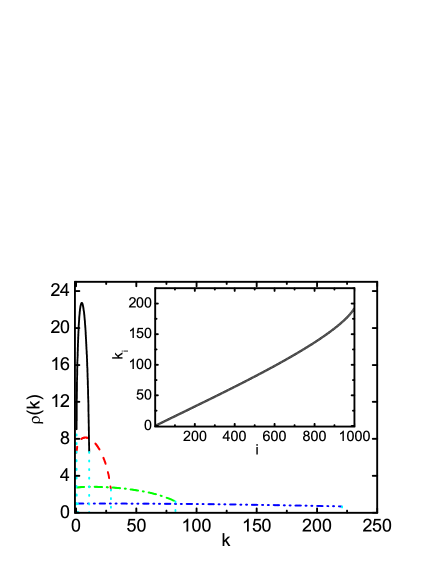
Figure 1: (color online) The density of state in quasi-momentum $k$ space for the ground state for $N=200$ and $c=0.1$ (solid line), $c=1$ (dashed lines), $c=10$ (dash dot lines), $c=100$ (dash dot dot lines). Inset: The numerical solutions of the Bethe ansatz equations for $N=1000$ and $c=10$.

We consider $N$ particles with the $\delta$ interaction in one dimensional box with length $L$. The Schrödinger equation can be formulated as (the natural unit is used)

$$\left[-\sum_{i=1}^{N}\frac{\partial^{2}}{\partial x_{i}^{2}}+2c\sum_{1\leq i<j\leq N}\delta\left(x_{i}-x_{j}\right)\right]\Psi=E\Psi,$$

where $2c$ is the interaction strength between atoms related with the $s$ -wave scattering length Olshanii ; Olshanii2 , which can be tuned from $-\infty$ to $+\infty$ by the Feshbach resonance or confinement induced resonance. When the interaction between atoms is repulsive, $c>0$, and in the attractive case $c<0$. The important parameter characterizing different physical regimes of 1D quantum gas is $\gamma=c\rho^{-1}$, where $\rho=N/L$. We will study the full physical regimes $-\infty<c<\infty$. The wavefunction can be written as

$$\Psi\left(x_{1},\cdots,x_{N}\right) = \sum_{P}\varphi\left(x_{p_{1}},x_{p_{2}},\cdots,x_{p_{N}}\right)$$

$$\times\theta\left(x_{p_{1}}<x_{p_{2}}\cdots<x_{p_{N}}\right),$$

in which

$$\theta\left(x_{p_{1}}<\cdots<x_{p_{N}}\right)=\theta\left(x_{p_{N}}-x_{p_{N-1}}\right)\cdots\theta\left(x_{p_{2}}-x_{p_{1}}\right),$$

$p_{1},p_{2},\cdots,p_{N}$ is one of the permutations of $1,\cdots,N$, and $\sum_{P}$ is the sum of all permutations. $\theta(x-y)$ is the step function. The wavefunction $\varphi\left(x_{p_{1}},x_{p_{2}},\cdots,x_{p_{N}}\right)$ could be obtained by the permutation of $\varphi\left(x_{1},\cdots,x_{N}\right)$ according to the symmetry condition of the Boson wave function. It turns out that the original problem is equivalent to solving the equation

$$\left[-\sum_{i=1}^{N}\frac{\partial^{2}}{\partial x_{i}^{2}}+2c\sum_{1\leq i<j\leq N}\delta\left(x_{i}-x_{j}\right)\right]\varphi\left(x_{1},\cdots,x_{N}\right)$$ (1)

$$= E\varphi\left(x_{1},\cdots,x_{N}\right)$$

in the region $0\leq x_{1}\leq x_{2}\leq\cdots\leq x_{N}\leq L$. We take the wave function $\varphi\left(x_{1},\cdots,x_{N}\right)$ as the Bethe ansatz type

$$\varphi\left(x_{1},x_{2},\cdots,x_{N}\right)=\sum_{P,r_{1},\ldots,r_{N}}\left[A_{P}\exp\left(i\sum_{j}r_{j}k_{p_{j}}x_{j}\right)\right],$$ (2)

where $r_{j}=\pm$ indicates that the particles move toward the right or the left. Substituting eq.(2) into eq.(1) and using the open boundary conditions

$$\varphi\left(0,x_{2},\cdots,x_{N}\right)=\varphi\left(x_{1},x_{2},\cdots,L\right)=0,$$

we have the Bethe ansatz equations

$$\exp\left(i2k_{j}L\right)=\prod_{l=1\left(\neq j\right)}^{N}\frac{ik_{l}+ik_{j}-c}{ik_{l}+ik_{j}+c}\frac{ik_{l}-ik_{j}+c}{ik_{l}-ik_{j}-c},$$ (3)

with $j=1,2,\cdots,N$. The energy eigenvalue is $E=\sum_{j=1}^{N}k_{j}^{2}$ and the total momentum is $k=\sum_{j=1}^{N}k_{j}$.

Taking the logarithm of Bethe ansatz equations, we have

$$k_{j}L=n_{j}\pi+\sum_{l=1\left(\neq j\right)}^{N}\left(\arctan\frac{c}{k_{j}+k_{l}}+\arctan\frac{c}{k_{j}-k_{l}}\right)$$ (4)

with $j=1,\cdots,N$. Here $\left\{n_{j}\right\}$ is a set of integer which determines an eigenstate and for the ground state $n_{j}=1$ ($1\leq j\leq N$). Alternatively, eq. (4) has the form of

$$k_{j}L=n_{j}^{\prime}\pi-\sum_{l=1\left(\neq j\right)}^{N}\left(\arctan\frac{k_{j}+k_{l}}{c}+\arctan\frac{k_{j}-k_{l}}{c}\right).$$ (5)

The above two equations are consistent but the choice of $\left\{n_{j}^{\prime}\right\}$ is different from that of $\left\{n_{j}\right\}$. For the latter case, we should have $n_{j}^{\prime}=j$ ($1\leq j\leq N$ ) for the ground state. The $\left\{k_{j}\right\}$, and thus the wave function can be decided by the set of transcendental equations eqs.(4). In general, the eqs.(5) are used in the literature Takahashi ; Korepin for the model with repulsive interaction, because it is more convenient to extend it to deal with the problem of thermodynamics. For $c>0$, the set of $k_{i}$ is unique and real, therefore the density of state in $k$ space $\rho(k)$ can be formulated as Yang

$$L\rho\left(\frac{k_{j}+k_{j+1}}{2}\right)=\frac{1}{k_{j+1}-k_{j}}.$$ (6)

However, such a definition does not make sense when $c<0$. In the later, through an example with $N=3$, we will show that in the attractive case the solution is not unique corresponding to a given set of $\left\{n_{j}\right\}$ and the ground state is decided by comparing the energy eigenvalues of different solutions.

With some algebraic calculation, the wave function has the following explicit form

$$\varphi\left(x_{1},x_{2},\cdots,x_{N}\right)$$

$$= \sum_{P}A_{p}\in_{p}\exp\left[i\left(\sum_{l<j}^{N-1}\omega_{p_{j}p_{l}}\right)\right]\exp\left(ik_{p_{N}}L\right)\sin\left(k_{p_{1}}x_{1}\right)$$

$$\times\prod_{1<j<N}\sin\left(k_{p_{j}}x_{j}-\sum_{l<j}\omega_{p_{l}p_{j}}\right)\sin\left(k_{p_{N}}\left(L-x_{N}\right)\right)$$

with

$$\omega_{ab}=\arctan\frac{c}{k_{b}-k_{a}}+\arctan\frac{c}{k_{b}+k_{a}}$$

and

$$A_{p_{1}p_{2}...p_{N}}=\prod_{j<l}^{N}\left(ik_{p_{l}}-ik_{p_{j}}+c\right)\left(ik_{p_{l}}+ik_{p_{j}}+c\right).$$

Here $\in_{p}$ denotes a $+(-)$ sign factor associated with even (odd) permutations. In terms of the ground state wave function $\Psi\left(x_{1},\cdots,x_{N}\right)$, the one body density matrix is defined as

$$\rho(x)=\frac{N\int_{0}^{L}dx_{2}\cdots dx_{N}\left|\Psi\left(x,x_{2},x_{3},\cdots,x_{N}\right)\right|^{2}}{\int_{0}^{L}dx_{1}\cdots dx_{N}\left|\Psi\left(x_{1},x_{2},\cdots,x_{N}\right)\right|^{2}}.$$

In the following calculation, we will let $L=1$ through the paper. Firstly, the repulsive interaction case is considered. The density of ground state in quasi-momentum $k$ space for different interaction constants is plotted in Fig. 1. It is shown that the density is suppressed for $k$ close to zero because of the confinement by the infinite-depth well. The numerical results of eqs. (4) are given for $N=1000$ and $c=10$ in the inset. Bethe ansatz equations uniquely decide the value of $k_{i}$, the wave function of the ground state and the one body density matrix of the system. In Fig. 2, we show the one body density matrix of the ground state for $N=4$ for different interaction constant. When there is no interaction between atoms ($c=0$), all of the atoms have the same quasi momentum, $k_{j}=\pi$ ($1\leq j\leq N$), corresponding to condensation of the ideal Bose gas. The one body density matrix is the sum of the density of $N$ independent bosonic atoms lying in the ground state. As the interaction increases further, the half-width of the density of the system becomes larger and larger with increasing interaction. At $c=10$, the density distribution shows already Fermion-like behavior. As the further increase of interaction the Bosons display the same density profile as that of $N$ noninteracting spinless Fermions and we have $k_{j}\simeq j\pi$ ($1\leq j\leq N$) at $c\sim 1000$.

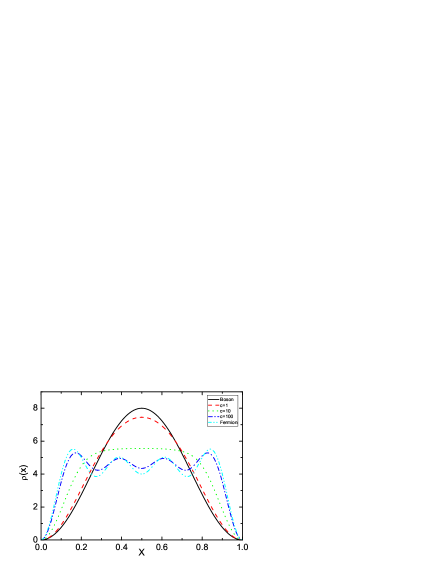
Figure 2: (color online) The density profiles $\rho(x)$ of the ground state for different repulsive interaction constants and $N=4$.

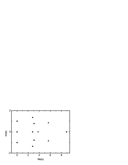
Figure 3: Three sets of solution (squares,triangles,circles) for 3 Bosons in a hard-wall trap with the attractive interaction $c=-1$. As comparison, diamonds correspond to the ground state solution of a periodic 3-Boson system on a ring of length $L=1$ for $c=-1$.

In the case of attractive interaction, $c<0$, eqs. (4) have solutions with complex quasi-momentum. The case for periodical boundary condition has been investigated in reference Takahashi ; Muga98 ; Sakmann . Due to the zero-point energy for a confined system, the solution corresponding to the ground state is not purely imaginary like that for the Bethe ansatz equations with periodical boundary condition. For the two body problem, the complex solutions of the Bethe ansatz equations take the form of the two-string solution

$$k_{1} = \alpha-i\Lambda,$$

$$k_{2} = \alpha+i\Lambda,$$

where $\alpha$ and $\Lambda$ are real and $2\alpha$ is the momentum of the system. In general, by an $N$-string solution we mean a solution where $N$ momenta $k_{i}$ possess the same real part. Then the eqs. (4) have the following form

$$\alpha L = \frac{n_{1}+n_{2}}{2}\pi+\arctan{\frac{c}{2\alpha},}$$

$$\Lambda L = \frac{1}{2}\ln\frac{2\Lambda-c}{2\Lambda+c},$$ (7)

where $n_{1}=n_{2}=1$ for the ground state. The corresponding energy of the system is $E=2\alpha^{2}-2\Lambda^{2}$. In terms of the momentum $k=2\alpha$, the energy can be represented as $E=k^{2}/2-2\Lambda^{2}$, which implies that the state corresponding to a two-string solution can be regarded as a bound state of two atoms with a binding energy $-2\Lambda^{2}$ and a doubled mass. For convenience, we also refer to the bound state corresponding to a two-string solution as a dimer state in the following text.

For the three-body problem, we assume that the solution has the following form: $k_{1}=\alpha-i\Lambda,$ $k_{2}=\alpha+i\Lambda$ and $k_{3}=\beta,$ therefore the Bethe ansatz equations can be represented with $\alpha$, $\beta$ and $\Lambda$. For the case with periodic boundary condition, there exists a 3-string solution corresponding to $\alpha=\beta$, i.e. the trimer state (the bound state of three particles) Takahashi ; Muga98 . But we can prove that no 3-string solution could be formed in a box for finite attractive interaction (see the appendix for details). That means the open boundary condition or a confinement tends to prevent the formation of a trimer state. We show the solutions of three-body problem for periodical boundary condition (Diamonds) and open boundary condition (Squares,Triangles and Circles denoting three sets of different solutions) for $c=-1$ in Fig. 3. It should be noticed that the set of solution denoted with squares is not an exact 3-string solution although $\alpha\approx\beta$, which is a dimer plus a single atom. By comparing $E$, the trimer-like solution (squares) has the lowest energy eigenvalue and thus it represents the ground state of the system.

Figure 4: The solutions to the Bethe ansatz equations for $N=10$ with different attractive interaction constants. $c$ takes the value of $-10$, $-4.0$, $-3.0$, $-2.0$, $-1.8$, $-1.6$, $-1.4$, $-1.2$, $-1.1$, $-1.0$, $-0.9$, $-0.8$, $-0.7$, $-0.6$, $-0.5$ (from left to right). Inset: (a) $c=-0.8$; (b) $c$ takes the values of $-0.4$, $-0.3$, $-0.2$, $-0.1$ (from left to right).

For the system with four atoms, the general complex solutions can be assumed as $k_{1}=\alpha-i\Lambda_{1},$ $k_{2}=\alpha+i\Lambda_{1},$ $k_{3}=\beta-i\Lambda_{2}$ and $k_{4}=\beta+i\Lambda_{2}$. By solving the Bethe ansatz equations numerically, it turns out that the ground state corresponds to a string solution of length four ($\alpha=\beta$ but $\Lambda_{1}\neq\Lambda_{2}$) for the large attractive interaction, whereas the ground state is a scattering state of two dimers for the weak attractive interaction. For $N>4$ the numerical results show that generally the ground state of the system in the weak attractive regime is a scattering state of $N/2$ dimers ($N$ is even) or $(N-1)/2$ dimers plus a single atom ($N$ is odd). The state of $N/2$ dimers is given in terms of $N/2$ two-string solutions. As the attractive interaction increases further, the ground state smoothly evolves into an intermediate regime characterized by an $(N-M)$-string solution plus $M/2$ two-string solutions with $2\leq M\leq N$, and finally it falls into the strong coupling regime corresponding to the $N$-string solution. To give an explicit example, we display the ground state solutions to the eqs.(4) for $N=10$ with different finite attractive interactions in Fig. 4. Based on the numerical solutions of the Bethe ansatz equations, we find that $5$ dimers form the ground state of the system when the attractive interaction is weak ($-1.42<c<0$). While in the limit of strong attractive interaction($c\leq-3.02$), the ground state solution is a 10-string solution. In the intermediate regime ($-3.02<c\leq-1.42$), the ground state solution is composed of a 4-string solution plus three 2-string solutions for $-1.72<c\leq-1.42$, a 6-string solution plus two 2-string solutions for $-1.88<c\leq-1.72$, and an 8-string solution plus a 2-string solution for $-3.02<c\leq-1.88$.

For the periodic system, the $N$-string ansatz is represented as

$$k_{j}=\alpha+i(N+1-2j)(c/2),~{}~{}~{}~{}j=1,\cdots,N.$$

The N-string ansatz is generally believed to be the solution of the Bethe ansatz equations for $c<0$ in the limit $L\rightarrow\infty$Takahashi . For the Bose gases in a finite-size hard-wall trap, we assume that the $N$-string solution takes the following form

$$k_{j}=\alpha+i(N+1-2j)(c/2+\delta_{j}),~{}~{}~{}~{}j=1,\cdots,N,$$ (8)

where ${\delta_{j}}$ is a set of small numbers and $\delta_{j}\rightarrow 0$ as $c\rightarrow-\infty$. Our numerical solutions to eqs.(4) indicate that the solutions are precisely fitted by the $N$-string ansatz of eqs.(8) in the limit of large attractive interaction. For instance, for the system with ten atoms the solution takes the values of $k_{j}=0.498075-i(11-2j)(5+\delta_{j})$ with $|\delta_{j}|<10^{-8}$ for $c=-3.02$ and $k_{j}=0.354213-i(11-2j)(5+\delta_{j})$ with $|\delta_{j}|<10^{-13}$ for $c=-10$. In the strong attractive limit, we can determine $\alpha$ analytically. With eq. (8) and the original Bethe ansatz equations the total momentum can be formulated as

$$\exp\left(i2kL\right)=\prod_{1\leq j<N}\left[\frac{2\alpha+i(jc)}{2\alpha-i(jc)}\right]^{2},$$

where $k=N\alpha$ and we have taken $\delta_{i}=0$. Taking the logarithm to the above equation, we have

$$kL=n\pi+\sum_{1\leq j<N}2\arctan\frac{jc}{2\alpha},$$ (9)

where $n=N$ for the ground state. It is clear that the momentum $k$ is $\pi$ in the limit of $c\rightarrow-\infty$ and therefore $\alpha=\pi/N$ in the strong attractive limit.

In Fig. 5 we plot the one body density matrix of the ground state for $N=2$ (a) and $N=4$ (b). It is shown that as the attractive interaction increases, the central density of the system becomes large firstly and then less. In the limit of $c\rightarrow-\infty$ ($c\sim-1000$ for $N=2$), the density profile matches the case of $c=0$. The matching between them can be explained as a compounded particle with mass $Nm$ located in its ground state, whose density distribution has the form of $\sin^{2}x$ in the strong attractive limit. When the solution of Bethe ansatz equations take the form of eq.(8), the ground state energy can be represented as $E=k^{2}/N-N(N^{2}-1)c^{2}/12$, which implies that the state corresponding to the $N$-string solution can be regarded as a bound state of $N$ atoms with a binding energy $\propto-c^{2}$ and a mass $N$m. It is also interesting to study the second order correlation function

$$g_{2}(x,c)=\frac{N(N-1)\int_{0}^{L}dx_{3}\cdots dx_{N}\left|\Psi\left(x,x,x_{3},\cdots,x_{N}\right)\right|^{2}}{\int_{0}^{L}dx_{1}\cdots dx_{N}\left|\Psi\left(x_{1},x_{2},\cdots,x_{N}\right)\right|^{2}}.$$

In Fig. 6 we show the dependence of second-order correlation function upon the interaction. It indicates that the atoms tend to cluster together more easily for the attractive interaction and the atoms bunch closer as the interaction becomes stronger. For the repulsive interactions, the atoms avoid each other and the atom-bunching reduces and vanishes finally for increasing interactions, which is similar to the case for the periodical boundary condition Shlyapnikov .

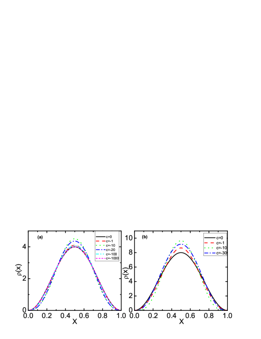
Figure 5: (color online) The density profiles $\rho(x)$ of the ground state for different attractive interaction constants. (a) $N=2$ and (b) $N=4$.

Figure 6: The second-order correlation function versus $c$ for $N=4$. Inset: The second-order correlation function for repulsive interaction with $N=4$.

In conclusion, by numerically solving the Bethe ansatz equations we investigate the ground state properties and obtain the density distribution function and the second-order correlation function of the 1D Bose gases in a box of finite length $L$ in all the physical regimes ($-\infty<c<+\infty$). In the limit of $c\rightarrow\infty$ the Bose gas shows similar behavior as that of noninteracting spinless Fermions, while in the limit of $c\rightarrow-\infty$ the Bose gas behaves as a compounded particle with mass $Nm$. In the case of weakly attractive interaction the ground state is composed of $N/2$ dimers ($N$ is even) or $(N-1)/2$ dimers plus a single atom ($N$ is odd). The second-order correlation function indicates that the atoms bunch closer as the interacting constant $c$ decreases. Our results can cover the whole parameter regime beyond the mean field theory and display the continuous crossover behavior from the Tonks limit to the strongly attractive limit. Especially, the crossover behavior of the ground state for the case of attractive interactions is discussed in detail. Hopefully, our results based on the exact solution can provide a clear picture of the wavefunction for the BECs with attractive interaction in a trap and help us to gain some intuitive insight on the collapse of BEC.

S.C. would like to acknowledge helpful discussions with Y. Wang, W. D. Li and S. J. Gu. He also thanks the Chinese Academy of Sciences for financial support. This work is supported in part by NSF of China under Grant No. 10574150. Y.Z. thanks the hospitality of Prof. K.-A. Suominen and the Quantum Optics group for their hospitality at University of Turku, where some of this work was done. He is also supported by Shanxi Province Youth Science Foundation under grant No. 20051001.

Appendix A The string solution for the attractive three-atom system

In this appendix, we study the three-particle system in detail. We firstly assume the 3-string solution for 3-atom system in the form of $k_{1}=\alpha-i\Lambda,$ $k_{2}=\alpha+i\Lambda$ and $k_{3}=\alpha.$ In terms of $\alpha$ and $\Lambda,$ then the Bethe ansatz equations take the following forms

$$\exp\left[\left(i2\alpha+2\Lambda\right)L\right]$$

$$= \frac{i2\alpha+\Lambda-c}{i2\alpha+\Lambda+c}\frac{i2\alpha-c}{i2\alpha+c}\frac{\Lambda-c}{\Lambda+c}\frac{2\Lambda-c}{2\Lambda+c},$$

$$\exp\left[\left(i2\alpha-2\Lambda\right)L\right]$$

$$= \frac{i2\alpha-c}{i2\alpha+c}\frac{i2\alpha-\Lambda-c}{i2\alpha-\Lambda+c}\frac{2\Lambda+c}{2\Lambda-c}\frac{\Lambda+c}{\Lambda-c},$$

$$\exp\left[i2\alpha L\right]$$

$$= \frac{i2\alpha+\Lambda-c}{i2\alpha+\Lambda+c}\frac{i2\alpha-\Lambda-c}{i2\alpha-\Lambda+c},$$ (12)

where we have used $\frac{\Lambda+c}{\Lambda-c}\frac{\Lambda-c}{\Lambda+c}=1$ in the right of the third equation. Substituting eq. (A3) into (A1) and (A2), we then get

$$\exp\left[2\Lambda L\right]\frac{i2\alpha-\Lambda-c}{i2\alpha-\Lambda+c} = \frac{i2\alpha-c}{i2\alpha+c}\frac{\Lambda-c}{\Lambda+c}\frac{2\Lambda-c}{2\Lambda+c},$$

$$\exp\left[-2\Lambda L\right]\frac{i2\alpha+\Lambda-c}{i2\alpha+\Lambda+c} = \frac{i2\alpha-c}{i2\alpha+c}\frac{2\Lambda+c}{2\Lambda-c}\frac{\Lambda+c}{\Lambda-c}.$$

The above two equations can be rewritten as

$$\exp\left[2\Lambda L\right]\sqrt{\frac{4\alpha^{2}+\left(\Lambda+c\right)^{2}}{4\alpha^{2}+\left(\Lambda-c\right)^{2}}}$$

$$\times\exp\left[i\left(\arctan\frac{\Lambda+c}{2\alpha}-\arctan\frac{\Lambda-c}{2\alpha}\right)\right]$$

$$= \exp\left[2i\arctan\frac{c}{2\alpha}\right]\frac{\Lambda-c}{\Lambda+c}\frac{2\Lambda-c}{2\Lambda+c},$$

$$\exp\left[-2\Lambda L\right]\sqrt{\frac{4\alpha^{2}+\left(\Lambda-c\right)^{2}}{4\alpha^{2}+\left(\Lambda+c\right)^{2}}}$$

$$\times\exp\left[i\left(\arctan\frac{\Lambda+c}{2\alpha}-\arctan\frac{\Lambda-c}{2\alpha}\right)\right]$$

$$= \exp\left[2i\arctan\frac{c}{2\alpha}\right]\frac{2\Lambda+c}{2\Lambda-c}\frac{\Lambda+c}{\Lambda-c}.$$

Comparing the module or imaginary part of the left and right side of these two equations, we can get three equations corresponding to Eqs. (A1), (A2) and (A3)

$$\exp\left[2\Lambda L\right]=\sqrt{\frac{4\alpha^{2}+\left(\Lambda-c\right)^{2}}{4\alpha^{2}+\left(\Lambda+c\right)^{2}}}\frac{\Lambda-c}{\Lambda+c}\frac{2\Lambda-c}{2\Lambda+c},$$ (13)

$$\exp\left[2i\arctan\frac{c}{2\alpha}\right]$$

$$= \exp\left[i\left(\arctan\frac{\Lambda+c}{2\alpha}-\arctan\frac{\Lambda-c}{2\alpha}\right)\right],$$

$$\exp\left[i2\alpha L\right]$$

$$= \exp\left[2i\left(\arctan\frac{\Lambda+c}{2\alpha}-\arctan\frac{\Lambda-c}{2\alpha}\right)\right].$$ (15)

Observing that there are two unknown parameters $\alpha$ and $\Lambda$ but they need fulfill three equations, there are no solutions to the above equations for an arbitrary $c$. This means that the three-string assumption is not a solution to the Bethe ansatz equations. Also, we have solved the above equations numerically, but no solutions are found.

Next we assume that the solution for a 3-atom system has the following form $k_{1}=\alpha-i\Lambda,$ $k_{2}=\alpha+i\Lambda$ and $k_{3}=\beta$ with $\Lambda>0$. With similar procedure as above, the Bethe ansatz equations can be represented as

$$\left(2\alpha+\beta\right)L = \left(2n+n^{\prime}\right)\pi+2\left(\arctan\frac{\Lambda+c}{\alpha+\beta}\right.$$ (16)

$$\left.-\arctan\frac{\Lambda-c}{\alpha+\beta}+\arctan\frac{c}{2\alpha}\right),$$

$$\left(2\alpha-\beta\right)L = \left(2n-n^{\prime}\right)\pi+2\left(\arctan\frac{\Lambda+c}{\alpha-\beta}\right.$$ (17)

$$\left.-\arctan\frac{\Lambda-c}{\alpha-\beta}+\arctan\frac{c}{2\alpha}\right),$$

$$\exp\left[2\Lambda L\right] = \frac{\left[\left(\alpha+\beta\right)^{2}+\left(\Lambda-c\right)^{2}\right]^{1/2}}{\left[\left(\alpha+\beta\right)^{2}+\left(\Lambda+c\right)^{2}\right]^{1/2}}$$ (18)

$$\frac{\left[\left(\alpha-\beta\right)^{2}+\left(\Lambda-c\right)^{2}\right]^{1/2}}{\left[\left(\alpha-\beta\right)^{2}+\left(\Lambda+c\right)^{2}\right]^{1/2}}\frac{2\Lambda-c}{2\Lambda+c}.$$

where $n$ and $n^{\prime}$ are integers which can be determined in the limit $c\rightarrow 0$. Here $\left(2\alpha+\beta\right)$ corresponds to the total momentum which is conserved in the periodic boundary condition case, but not in the open boundary case. We will see that $n=n^{\prime}=1$ corresponds to the ground state. For the limit $c=0$, we have $2\alpha+\beta=3\pi/L$ which means that three atoms all occupy the lowest energy level. In the other limit $c\rightarrow-\infty$, it is not obvious. By numerically solving the Bethe ansatz equations, we can get the values of $\alpha$, $\beta$ and $\Lambda$. Corresponding to $n=n^{\prime}=1$, we get three sets of solution as shown in Fig. 3. Among the three solutions, we get $2\alpha+\beta=\pi/L$ corresponding to the solution $\Lambda=-c+\delta$ (the solution denoted by squares in Fig. 3), where $\delta$ is a small number in the large $c$ limit. This solution is the trimer-like solution describing the ground state of the attractive 3-atom system.

References

- (1) A. Görlitz, et.al., Phys. Rev. Lett. 87, 130402 (2001).
- (2) H. Moritz, T. Stöferle, M. Köhl, and T. Esslinger, Phys. Rev. Lett. 91, 250402 (2003); T. Stöferle, H. Moritz, C. Schori, M. Köhl, and T. Esslinger, ibid. 92 , 130403 (2004).
- (3) B. Paredes, A. Widera, V. Murg, O. Mandel, S. Fölling, I. Cirac, G. V. Shlyapnikov, T. W. Hänsch, and I. Bloch, Nature 429, 277 (2004).
- (4) T. Kinoshita, T. Wenger and D. S. Weiss, Science 305, 1125 (2004).
- (5) B. L. Tolra, K. M. O’Hara, J. H. Huckans, W. D. Phillips, S. L. Rolston, and J. V. Porto, Phys. Rev. Lett. 92, 190401 (2004).
- (6) N. J. van Druten and W. Ketterle, Phys. Rev. Lett. 79, 549 (1997).
- (7) M. Olshanii, Phys. Rev. Lett. 81, 938 (1998).
- (8) M. D. Girardeau, J. Math. Phys. (N.Y.) 1, 516 (1960); L. Tonks, Phys. Rev. 50, 955 (1936).
- (9) K. K. Das, G. J. Lapeyre, and E. M. Wright, Phys. Rev. A. 65, 063603 (2002).
- (10) T. Bergeman, M. G. Moore, and M. Olshanii, Phys. Rev. Lett. 91, 163201 (2003).
- (11) P. Öhberg and L. Santos, Phys. Rev. Lett. 89, 240402 (2002).
- (12) D. S. Petrov, G. V. Shlyapnikov, and J. T. M. Walraven, Phys. Rev. Lett. 85, 3745 (2000).
- (13) V. Dunjko, V. Lorent and M. Olshanii, Phys. Rev. Lett. 86, 5413 (2001).
- (14) D. L. Luxat and A. Griffin, Phys. Rev. A. 67, 043603 (2003).
- (15) P. Pedri, L. Santos, P. Öhberg, and S. Stringari, Phys. Rev. A. 68, 043601 (2003).
- (16) E. B. Kolomeisky, T. J. Newman, J. P. Straley, and X. Qi, Phys. Rev. Lett. 85, 1146 (2000).
- (17) S. Chen and R. Egger, Phys. Rev. A. 68, 063605 (2003).
- (18) M. D. Girardeau and E. M. Wright, Phys. Rev. Lett. 84, 5239 (2000); T.-L. Ho and M. Ma, J. Low Temp Phys. 115 , 61 (1999).
- (19) E. H. Lieb and W. Liniger, Phys. Rev. 130, 1605 (1963); E. H. Lieb, ibid. 130, 1616 (1963).
- (20) C. N. Yang and C. P. Yang, J. Math. Phys. 10, 1115 (1969).
- (21) V. E. Korepin, A. G. Izergin and N. M. Bogoliubov, Quantum Inverse Scattering Method and Correlation Functions. (Cambridge University Press, Cambridge 1993).
- (22) M. Takahashi, Thermodynamic of One-Dimensional Solvable Models. (Cambridge University Press, Cambridge 1999).
- (23) J. B. McGuire, J. Math. Phys. 5, 622 (1964).
- (24) P. A. Ruprecht, M. J. Holland, K. Burnett, and M. Edwards, Phys. Rev. A 51, 4704 (1995).
- (25) L. D. Carr, C. W. Clark, and W. P. Reinhardt, Phys. Rev. A 62, 063610 (2000); ibid., 62, 063611 (2000).
- (26) W. Hänsel et al., Nature 413, 498 (2001).
- (27) T. P. Meyrath, F. Schreck, J. L. Hanssen, C.-S. Chuu, and M. G. Raizen, Phys. Rev. A 71, 041604 (2005).
- (28) M. Gaudin, Phys Rev. A 4, 386 (1971).
- (29) M.T. Batchelor, X.W. Guan, N. Oelkers, and C. Lee, J. Phys. A: Math. Gen. 38, 7787 (2005).
- (30) N. Oelkers, M.T. Batchelor, M. Bortz, X.W. Guan, J. Phys. A: Math. Gen. 39, 1073 (2006).
- (31) S. Gu, Y. Li and Z. Ying, J. Phys. A: Math. Gen. 34, 8995 (2001).
- (32) A. del Campo and J. G. Muga, cond-mat/0511747.
- (33) J. G. Muga and R. F. Snider, Phys. Rev. A 57, 3317 (1998).
- (34) K. Sakmann, A. I. Streltsov, O. E. Alon, and L. S. Cederbaum, Phys. Rev. A 72, 033613 (2005).
- (35) D. M. Gangardt and G.V. Shlyapnikov, Phys. Rev. Lett 90, 010401 (2003).