Nonlocal Homogenization Model for a Periodic Array of $\epsilon$-Negative Rods

Abstract

We propose an effective permittivity model to homogenize an array of long thin $\epsilon$-negative rods arranged in a periodic lattice. It is proved that the effect of spatial dispersion in this electromagnetic crystal cannot be neglected, and that the medium supports dispersionless modes that guide the energy along the rod axes. It is suggested that this effect may be used to achieve sub-wavelength imaging at the infrared and optical domains. The reflection problem is studied in detail for the case in which the rods are parallel to the interfaces. Full wave numerical simulations demonstrate the validity and accuracy of the new model.

I Introduction

In recent years there has been a lot of interest in the propagation of electromagnetic waves in artificial materials, and particularly in materials with negative index of refraction Veselago (1968); Shelby et al. (2001). The research has been mainly driven by the possibility of using these materials to miniaturize several devices and waveguides, and develop ”perfect lenses” able of focusing electromagnetic radiation with sub-wavelength resolution Pendry (2000). Recently, a different approach to achieve sub-wavelength resolution was proposed in Belov et al. (2005) and demonstrated experimentally in Belov et al. (2006). In Belov et al. (2006) the idea is to use an artificial material formed by an array of perfectly conducting wires (wire medium) to guide the waves from the input plane to the output plane, and then reconstruct the image ”pixel by pixel”, exploring a Fabry-Perot resonance that in the wire medium occurs simultaneously for all the spatial harmonics. The resolution of this transmission device is only limited by the lattice constant, i.e. by the spacing between the wires. The problem with the configuration studied in Belov et al. (2006) is that it is limited to the microwave regime because in the optical domain perfect electric conducting materials are not available. Nevertheless, we will suggest in this paper that it may still be possible to use the same concept to achieve sub-wavelength resolution at the infrared and optical domains, provided $\epsilon$-negative (ENG) rods are used to guide the electromagnetic radiation instead of metallic wires. At the infrared and optical frequencies all metallic materials have permittivity with negative real part. It is known that their dielectric constant is well represented by the Drude model $\epsilon=1-\omega_{p}^{2}/\omega^{2}$, where $\omega_{p}$ is the plasma frequency (for simplicity the lossless model was considered). Thus, we envision that either silver or gold rods may used to fabricate transmission devices that are able to propagate the subwavelength information of an image.

With this motivation, we will investigate in this paper the propagation of electromagnetic waves in an artificial medium formed by thin ENG rods (see Fig. 1), and we will show that the structure can be homogenized and described by an effective permittivity tensor provided spatial dispersion is taken into account. We will show that our homogenization model predicts that the rod medium may support a mode that propagates along the axes of the rods with the same phase velocity, independently of the transverse wave vector. As proved in Belov et al. (2005), this is a key property to operate the material in the canalization regime and achieve sub-wavelength resolution.

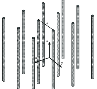
Figure 1: Medium formed by long thin ENG rods arranged in a square lattice.

Previous works related with the homogenization of ENG rods are discussed next. In Poulton et al. (2004) the oblique propagation of electromagnetic waves through an array of aligned fibres was examined, and the associated problem of numerical instability discussed. In Pokrovsky (2004) a method was proposed to compute analytically the band structure of wire mesh crystals. In Pokrovsky and Efros (2002a) a model was proposed to homogenize a medium with metallic rods, but only the on-plane case was considered. In Pokrovsky and Efros (2002b) an homogenization model was proposed to characterize a structure similar to the one studied in this paper. It was demonstrated that the artificial material was characterized by spatial dispersion, and that the band structure of the photonic crystal had several branches. However, the results of Pokrovsky and Efros (2002b) are restricted to the case in which the permittivity of the rods follows a Drude-type plasma model, and besides that the derived formulas for the effective permittivity are very cumbersome, lead to non-analytical dispersion characteristics, and more importantly hide the physics of the problem. In this paper, we will derive a simpler and more intuitive model, describe new phenomena, and prove that the new approach can characterize accurately the electrodynamics of the artificial medium.

The homogenization of the wire medium is also closely related with the subject under study. In fact, the case of perfectly conducting wires can be regarded as the limit situation in which the permittivity of the ENG rods is $-\infty$. In Belov et al. (2003) an homogenization model was derived for the wire medium, and it was proved that this artificial material suffers from strong spatial dispersion even for very long wavelengths. Later, in Silveirinha and Fernandes (2005a); Simovski and Belov (2004), these results were generalized for 2D- and 3D lattices of connected and unconnected wires. In Silveirinha and Fernandes (2005b); Belov et al. (2002) the reflection problem in a wire medium slab was investigated, and in Silveirinha (2005) it was proved that in general an additional boundary condition is necessary to determine the scattering parameters.

The paper is organized as follows. Firstly, we will characterize the electric polarizability of a dielectric rod. Then, we will derive the homogenization rudiments necessary to calculate the effective permittivity of the structure. In section IV, the electromagnetic modes supported by the rod medium are characterized. In section V, we study the reflection problem in a finite slab, assuming that the rods are parallel to the interfaces. The derived results are compared with full wave numerical simulations. Finally, in section VI the conclusions are presented.

In this work we assume that the fields are monochromatic with time variation $e^{+j\omega t}$.

II Polarizability of a dielectric rod

Let us consider a ENG rod with radius $R$ and (relative) permittivity $\epsilon=\epsilon(\omega)$. The rod is oriented along the $z$-direction. In this section, we calculate the component $\alpha_{zz}$ of the electric polarizability tensor (actually, since the rod is infinite along $z$, we are going to calculate the polarizability per unit of lenght). To this end, we consider that a plane wave with magnetic field along the $y$-direction illuminates the dielectric rod. The wave vector of the incident wave is ${\bf k}=(k_{x},0,k_{z})$, where ${\bf{k}}{\bf{.k}}=\beta^{2}$ and $\beta=\omega/c$ is the free-space wave number. The incident electric field along the $z$-direction is:

$$E_{z}^{inc} =E_{0}e^{-j\,k_{x}x}e^{-j\,k_{z}z}$$

$$=E_{0}e^{-j\,k_{z}z}\sum\limits_{n=-\infty}^{\infty}{\left({-j}\right)^{\left|n\right|}J_{\left|n\right|}\left({k_{\rho,0}r}\right)e^{jn\varphi}}$$

where $J_{n}$ is the $J$-Bessel Function of first kind and order $n$, $k_{\rho,0}=\sqrt{\beta^{2}-k_{z}^{2}}$, and $(r,\varphi)$ form a system of cylindrical coordinates attached to the rod axis.

The field components along $z$ can be expanded into cylindrical harmonics. For example,

$$E_{z}=\left\{\begin{array}[]{l}\sum\limits_{n=-\infty}^{\infty}{a_{n}J_{\left|n\right|}\left({k_{\rho,m}r}\right)e^{jn\varphi}e^{-j{\kern 1.0pt}k_{z}z}}{\rm{,}}\,\,r<R\\ E_{z}^{inc}+\sum\limits_{n=-\infty}^{\infty}{b_{n}H_{\left|n\right|}^{\left(2\right)}\left({k_{\rho,0}r}\right)e^{jn\varphi}e^{-j{\kern 1.0pt}k_{z}z}}{\rm{,}}r>R\\ \end{array}\right.$$ (2)

where $a_{n}$ and $b_{n}$ are the unknown coefficients of the expansion, $H_{n}^{\left(2\right)}=J_{n}-jY_{n}$ is the Hankel function of second kind and order $n$, and $k_{\rho,m}=-j\sqrt{k_{z}^{2}-\beta^{2}\varepsilon}$. The field $H_{z}$ has a similar expansion.

The transverse fields ${\bf{E}}_{||}$ and ${\bf{H}}_{||}$ (projections into the $xoy$ plane) can be written in terms of $E_{z}$ and $H_{z}$:

$${\bf{E}}_{||}=\frac{1}{{k_{\rho,i}^{2}}}\left({-jk_{z}\nabla_{||}E_{z}+j\beta\,{\bf{\hat{u}}}_{z}\times\nabla_{||}\eta_{0}H_{z}}\right)$$ (3)

$$\eta_{0}{\bf{H}}_{||}=\frac{1}{{k_{\rho,i}^{2}}}\left({-j\beta\,\varepsilon_{i}{\bf{\hat{u}}}_{z}\times\nabla_{||}E_{z}-jk_{z}\,\nabla_{||}\eta_{0}H_{z}}\right)$$ (4)

In the above, $\eta_{0}$ is the free-space impedance, $\nabla_{||}=\left({\frac{\partial}{{\partial x}},\frac{\partial}{{\partial y}},0}\right)$, $\varepsilon_{i}=\varepsilon$ and $k_{\rho,i}=k_{\rho,m}$ inside the rod, and $\varepsilon_{i}=1$ and $k_{\rho,i}=k_{\rho,0}$ outside.

The unknown coefficients can be calculated by imposing the continuity of the tangential electromagnetic fields (i.e. $E_{z}$, $E_{\varphi}$, $H_{z}$, $H_{\varphi}$) at the interface $r=R$.

The ($z$ component of the) electric dipole moment (per unit of length) is given by,

$$\frac{{p_{z}}}{{\varepsilon_{0}}} =\left({\varepsilon-1}\right)\int\limits_{r\leq R}{E_{z}\,ds}$$ (5)

$$=\left({\varepsilon-1}\right)2\pi R\,a_{0}\frac{{J_{1}\left({k_{\rho,m}R}\right)}}{{k_{\rho,m}}}e^{-jk_{z}z}$$

and so the polarizability per unit of length is,

$$\alpha_{zz} =\frac{{p_{z}}}{{\varepsilon_{0}\left.{E^{inc}}\right|_{x=y=0}}}$$ (6)

$$=\left({\varepsilon-1}\right)2\pi R\,\frac{{a_{0}}}{{E_{0}}}\frac{{J_{1}\left({k_{\rho,m}R}\right)}}{{k_{\rho,m}}}$$

This result shows that $a_{0}$ is the unique coefficient required to calculate the polarizability. Since Maxwell equations are separable in cylindrical coordinates, to calculate $a_{0}$ it is sufficient to impose the boundary conditions to the terms associated with the cylindrical harmonic $n=0$. It can be easily verified that the $n=0$ term of the magnetic field $H_{z}$ vanishes (this happens because $H_{z}^{inc}=0$ and $\frac{\partial}{{\partial\varphi}}=0$ for the $n=0$ harmonic). Thus, only the tangential components $E_{z}$ and $H_{\varphi}$ have non-trivial $n=0$ coefficients. Using (II)-(2) in (3)-(4), and imposing the continuity of the tangential fields, we find that,

$$a_{0}J_{0}\left({k_{\rho,m}R}\right)=b_{0}H_{0}^{\left(2\right)}\left({k_{\rho,0}R}\right)+E_{0}J_{0}\left({k_{\rho,0}R}\right)$$ (7)

$$a_{0}\frac{\varepsilon}{{k_{\rho,m}}}J^{\prime}_{0}\left({k_{\rho,m}R}\right)=b_{0}\frac{1}{{k_{\rho,0}}}{H^{\prime}_{0}}^{\left(2\right)}\left({k_{\rho,0}R}\right)+\frac{1}{{k_{\rho,0}}}E_{0}J^{\prime}_{0}\left({k_{\rho,0}R}\right)$$ (8)

where the prime ”^′” denotes the derivative of a function. Solving for $a_{0}$ we readily obtain:

$$a_{0}^{-1}= j\frac{{\pi k_{\rho,0}R}}{2E_{0}}\times\left({J_{0}\left({k_{\rho,m}R}\right){H^{\prime}_{0}}^{\left(2\right)}\left({k_{\rho,0}R}\right)}\right.$$ (9)

$$-\left.{\frac{{\varepsilon k_{\rho,0}}}{{k_{\rho,m}}}J^{\prime}_{0}\left({k_{\rho,m}R}\right)H_{0}^{\left(2\right)}\left({k_{\rho,0}R}\right)}\right)$$

Substituting this result in (6), we obtain the desired electric polarizability:

$$\alpha_{zz}^{-1}= j\frac{{k_{\rho,0}}}{4}\frac{1}{{\varepsilon-1}}\times\left({-k_{\rho,m}\frac{{J_{0}\left({k_{\rho,m}R}\right)}}{{J_{1}\left({k_{\rho,m}R}\right)}}H_{1}^{\left(2\right)}\left({k_{\rho,0}R}\right)}\right.$$ (10)

$$+\left.{\varepsilon k_{\rho,0}H_{0}^{\left(2\right)}\left({k_{\rho,0}R}\right)}\right)$$

In this work, we consider that the radius of the rods is always much smaller than the wavelength, or equivalently, $Rk_{\rho,0}<<1$. In these circumstances, (10) simplifies to,

$$\alpha_{zz}^{-1}\approx \frac{1}{{\left({\varepsilon-1}\right)\pi R^{2}}}\left[{1+j\frac{\pi}{4}\left({\varepsilon-1}\right)\left({k_{\rho,0}R}\right)^{2}}\right.$$

$$\left.{+\frac{1}{2}\left({\varepsilon-1}\right)\left({C+\log\left({\frac{{k_{\rho,0}R}}{2}}\right)}\right)\left({k_{\rho,0}R}\right)^{2}}\right]$$

where $C$ is the Euler constant. It is important to note that because the rods are infinitely long, the polarizability depends not only on the frequency of the incoming wave, but also on the wave vector component $k_{z}$. If $\epsilon$ approaches $-\infty$ the above result reduces to the case of perfectly conducting rods studied in Belov et al. (2002).

Proceeding similarly, we can obtain the well-known formula for the electric polarizability (per unit of length) in the transverse plane ($xoy$ plane):

$$\alpha_{xx}=\alpha_{yy}\approx\frac{{\varepsilon-1}}{{\varepsilon+1}}2\pi R^{2}$$ (12)

Provided the permittivity of the rods is not too close to the resonance $\epsilon=-1$ and the rods are very thin, the polarizability can be neglected in the transverse plane.

III Effective Permittivity Model

In the following, we derive an effective permittivity model for the medium formed by a periodic array of ENG rods. As depicted in Fig. 1, the rods are arranged in a square lattice and the spacing between the rods (lattice constant) is $a$. As is well-known, each electromagnetic (Floquet) mode in a periodic medium can be associated with a wave vector ${\bf{k}}=(k_{x},k_{y},k_{z})$. For convenience, we define ${\bf{k}_{||}}=(k_{x},k_{y},0)$.

To compute the effective permittivity we use the mixing formula :

$$\overline{\overline{\varepsilon}}=\overline{\overline{\bf{I}}}+\frac{1}{{{\rm{A}}_{{\rm{cell}}}}}\left({\overline{\overline{\alpha}}_{e}^{-1}-\overline{\overline{{\bf{C}}}}_{{\mathop{\rm int}}}}\right)^{-1}$$ (13)

where ${\rm{A}}_{{\rm{cell}}}=a^{2}$, $\overline{\overline{\bf{I}}}$ is the identity dyadic, the superscript ”-1” represents the inverse dyadic, and $\overline{\overline{{\bf{C}}}}_{{\mathop{\rm int}}}$ is the interaction dyadic calculated in Appendix B. The mixing formula is derived in Appendix A, and is valid under the condition that the dimensions of the cross-section are much smaller than the lattice constant, and that $|{\bf{k_{||}}}|a<<2\pi$. As discussed in Appendix A, even though (13) reminds Clausius-Mossotti formula, things are not so plain because the lattice has some intrinsic dispersion. To keep the readability of the paper the details have been moved to Appendix A.

Next we substitute (II) and (12) in (13). Using (47), we find that the effective permittivity in the transverse plane is

$$\varepsilon_{xx}=\varepsilon_{yy}=1+\frac{2}{{\frac{1}{{f_{V}}}\frac{{\varepsilon+1}}{{\varepsilon-1}}-1}}$$ (14)

where $f_{V}={{\pi R^{2}}\mathord{\left/{\vphantom{{\pi R^{2}}{{\rm{A}}_{{\rm{cell}}}}}}\right.\kern-1.2pt}{{\rm{A}}_{{\rm{cell}}}}}$ is the volume fraction of the rods. Provided the permittivity of the rods does not satisfy $\epsilon\approx-1$ and the rods are very thin, we can assume that $\epsilon_{xx}=\epsilon_{yy}\approx 1$. For simplicity, we shall assume this situation in the rest of the paper. On the other hand, from (13) it is clear that,

$$\varepsilon_{zz}=1+\frac{1}{{\rm{A}_{{\rm{cell}}}}}\frac{1}{{\alpha_{zz}^{-1}-C_{{\mathop{\rm int}},zz}}}$$ (15)

where ${C_{{\mathop{\rm int}},zz}}$ is given by (50). So, after further simplifications, we obtain that:

$$\varepsilon_{zz}=1+\frac{1}{{\frac{1}{{\left({\varepsilon-1}\right)f_{V}}}-\frac{{\beta^{2}-k_{z}^{2}}}{{\beta_{p}^{2}}}}}$$ (16)

where $\beta_{p}$ is the plasma wave number defined consistently with the results of Belov et al. (2002) for perfectly conducting wires:

$$\left({\beta_{p}a}\right)^{2} =\frac{{2\pi}}{{\ln\left({\frac{a}{{2\pi R}}}\right)+\frac{\pi}{6}+\sum\limits_{n=1}^{\infty}{\frac{1}{{\left|n\right|}}\frac{2}{{e^{2\pi\left|n\right|}-1}}}}}$$ (17)

$$\approx\frac{{2\pi}}{{\ln\left({\frac{a}{{2\pi R}}}\right)+0.5275}}$$

Note that in general $\epsilon$ is a function of frequency. Formula (16) gives the effective permittivity of an array of diluted ENG rods. The first important observation is that the medium is spatially dispersive. Indeed the permittivity depends not only on the frequency $\beta=\omega/c$, but also on the component of the wave vector parallel to the rods. This means that the medium is nonlocal, i.e. in the spatial domain the electric displacement vector and the electric field are related through a spatial convolution rather than by a multiplication. Secondly, we note that if the permittivity of the rods approaches $-\infty$, (16) reduces to the formula derived in Belov et al. (2003) for the wire medium, consistently with the observation made in the introduction of this paper. Finally, if we put $\beta=0$ and assume on-plane propagation, i.e. $k_{z}=0$, the effective permittivity simplifies to $\varepsilon_{zz}=1+\left({\varepsilon-1}\right)f_{V}$, which is the exact formula in the static the limit for non-dispersive dielectrics Sihvola (1999). Thus, very interestingly, formula (16) is in a certain sense the average of these two limit situations. Note that even though in this work our main interest is the analysis of ENG rods, the proposed model is also valid for dielectrics with positive real part of the permittivity. In the next sections, we characterize the electromagnetic modes supported by the rod medium and validate the model with numerical simulations.

IV Characterization of the electromagnetic modes

It is evident that the waves in the homogenized medium can be decomposed into transverse electric (TE) modes (electric field is normal to the axes of the ENG rods), and transverse magnetic (TM) modes (magnetic field is normal to the axes of the ENG rods). As explained in the previous section, we shall assume in this paper that $\epsilon_{xx}=\epsilon_{yy}\approx 1$ (i.e. that the rods are very thin, and that the permittivity of rods is not close to $\epsilon\approx-1$). Within this approximation, the TE-modes do not interact with the rods, and thus their dispersion characteristic is,

$$\beta^{2}=k^{2}$$ (18)

and the associated average electric field is (the propagation factor $e^{-j{\bf{k}}{\bf{.r}}}$ is implicit)

$${\bf{E}}_{{\rm{av}}}^{TE}\propto\frac{{{\bf{k}}_{||}\times{\bf{\hat{u}}}_{z}}}{{\left|{{\bf{k}}_{||}\times{\bf{\hat{u}}}_{z}}\right|}}$$ (19)

On the other hand, the TM-modes satisfy the characteristic equation:

$$k_{||}^{2}=\varepsilon_{zz}\left({\beta^{2}-k_{z}^{2}}\right)$$ (20)

The above equation cannot be solved explicitly as a function of $\beta$, because the permittivity of the rods is itself a function of $\beta$. The corresponding average electric field is (for $k_{z}\neq 0$):

$${\bf{E}}_{{\rm{av}}}^{TM}\propto\left({\frac{{{\bf{k}}_{||}}}{\beta}+\frac{{\beta^{2}-k^{2}}}{{\beta^{2}\varepsilon_{zz}-k^{2}}}\frac{{k_{z}}}{\beta}{\bf{\hat{u}}}_{z}}\right)$$ (21)

The associated magnetic field can be calculated using (29).

To understand better the nature of the TM-modes, next we study a reflection problem. Let us consider a semi-infinite rod medium illuminated from the air side with a plane wave. We analyze two different geometries, as depicted in Fig. 2.

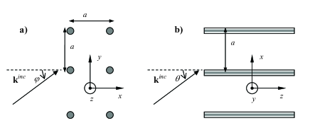
Figure 2: Reflection of a plane wave by a semi-infinite rod medium. a)The axes of the rods are parallel to the interface. b) The axes of the rods are normal to the interface.

Firstly, let us suppose that the axes of the rods are parallel to the interface $x=0$ (Fig. 2$a$). The incident wave vector is ${\bf{k}}^{inc}=(-j\gamma_{0},k_{y},k_{z})$ with $\gamma_{0}=\sqrt{k_{y}^{2}+k_{z}^{2}-\beta^{2}}$. It is well-known that the component of the incident wave vector parallel to the interface, $(0,k_{y},k_{z})$, is preserved. In this case only one TM-mode is excited in the artificial medium (besides the TE-mode). Indeed, from (20) the component $k_{x}$ of the wave vector inside the rod medium is given by:

$$k_{x,rod}^{2}=-k_{y}^{2}+\varepsilon_{zz}\left({\beta^{2}-k_{z}^{2}}\right)$$ (22)

Notice that the right-hand side of the above equation only depends on the geometry and parameters of the medium, on the wave number $\beta$ of the incident wave, and on the components of the incident wave vector that are preserved $(0,k_{y},k_{z})$.

Next suppose that the rods are normal to the interface $z=0$ (Fig. 2$b$). The incident wave vector is now ${\bf{k}}^{inc}=(k_{x},k_{y},-j\gamma_{0})$ with $\gamma_{0}=\sqrt{k_{x}^{2}+k_{y}^{2}-\beta^{2}}$. The interesting thing is that for this configuration two TM-modes can be excited inside the rod medium. Indeed, since ${\bf{k}_{||}}=(k_{x},k_{y},0)$ to find the excited electromagnetic modes one needs to solve (20) for $k_{z}$. Straightforward calculations, using (16), show that:

$$k_{z}^{2}= \beta^{2}-\frac{1}{2}\left({\beta_{p}^{2}+k_{||}^{2}-\beta_{c}^{2}}\right.$$ (23)

$$\left.{\pm\sqrt{\left({\beta_{p}^{2}+k_{||}^{2}-\beta_{c}^{2}}\right)^{2}+4\beta_{c}^{2}k_{||}^{2}}}\right)$$

where we defined the parameter $\beta_{c}=\beta_{c}(\omega)$ as,

$$\beta_{c}^{2}=-\frac{{\beta_{p}^{2}}}{{\left({\varepsilon\left(\omega\right)-1}\right)f_{V}}}$$ (24)

Note that provided the permittivity of the rods is less than the permittivity of the host medium, $\beta_{c}$ is a positive real number (with the same unities as $\beta$; for simplicity the rods are assumed lossless, otherwise $\beta_{c}$ becomes a complex number). Also, $\beta_{c}$ is in general a function of frequency since $\epsilon$ also is. From (23) it is seen that there are two different solutions for $k_{z}$, and hence two TM-modes, besides the TE-mode, can propagate inside the artificial medium. This phenomenon is a manifestation of spatial dispersion, and is also characteristic of the wire medium Belov et al. (2003). We also note that the average electric field for both TM-modes is calculated using (21).

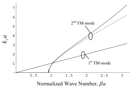
Figure 3: Plot of $k_{z}$ as a function of normalized frequency $\beta a$, for $R=0.05a$ and $k_{||}=0$. The permittivity $\epsilon$ follows a Drude type model (see the text). The solid line represents the ”exact” result, whereas the dashed line represents the results calculated with the proposed model.

To illustrate the discussion, we plot in Fig. 3, $k_{z}$ as a function of normalized frequency $\beta a$ for the parameters $R=0.05a$, $k_{||}=0$, assuming that the permittivity follows the Drude model $\epsilon=1-\beta_{m}^{2}/\beta^{2}$ with (normalized) plasma wave number $\beta_{m}a=12.0$. The dashed line curve represents the results calculated using (23). The solid line curve corresponds to the data calculated by substituting (10) in (15) (with no approximations) and calculating ${C_{{\mathop{\rm int}},zz}}$ using (48) with ${\bf{r}=\bf{r^{\prime}}}=0$, but without making any assumptions with respect to ${\bf{k}_{||}}a$ being negligible. Hence, the permittivity becomes a function of not only $\beta$ and $k_{z}$, but also of the other components of the wave vector. The permittivity function obtained in this way is substituted in (20), and the corresponding equation is solved numerically. A similar procedure was used in Pokrovsky and Efros (2002b); Belov et al. (2002), and so further details are omitted here. These results can be regarded as ”exact” within the thin rod approximation. As seen in Fig. 3, the agreement for the first TM-mode is always excellent. On the other hand, the second TM-mode is not so accurately predicted for relatively small wavelengths. The reason is twofold. The first reason is that for larger frequencies the long wavelength limit approximation is not so accurate. The second reason will be discussed later. Fig. 3 shows that for $k_{||}=0$ one of the electromagnetic modes propagates with the speed of light. It is also important to refer that for very low frequencies one of the TM-modes is cut-off (complex imaginary propagation constant). This is because the ENG rods behave as perfect conductors in the static limit (when the permittivity follows the Drude model).

To give further insight about the TM-modes, let us study different limit situations. First, suppose that at some frequency $\beta_{c}(\omega)<<\beta_{p}$, i.e. the permittivity of the rods is very large in absolute value. In this case, (23) reveals that one of the modes has the dispersion characteristic $k_{z}^{2}=\beta^{2}$, and that the other mode has the dispersion $k_{z}^{2}=\beta^{2}-\beta_{p}^{2}-k_{||}^{2}$. The former mode can be readily identified with the well-known transverse electromagnetic (TEM) dispersionless mode of the wire medium (perfectly conducting wires), while the latter is the TM-mode of the wire medium.

Consider now the case $\bf{k}_{||}\approx 0$, i.e. paraxial incidence. Using a Taylor expansion we obtain:

$$k_{z}^{2}\approx\beta^{2}+\frac{{k_{||}^{2}}}{2}\left({-1\pm\frac{{\beta_{c}^{2}+\beta_{p}^{2}}}{{\beta_{c}^{2}-\beta_{p}^{2}}}}\right)+\left\{\begin{array}[]{l}\beta_{c}^{2}-\beta_{p}^{2}\\ 0\\ \end{array}\right.$$ (25)

The above formula shows that if either $\beta_{c}(\omega)<<\beta_{p}$ or $\beta_{c}(\omega)>>\beta_{p}$, one of the modes becomes dispersionless with respect to $\bf{k}_{||}$ (i.e. the coefficient associated with $k_{||}^{2}$ vanishes). The former case was already discussed. As to the latter case, the pertinent mode has dispersion $k_{z}^{2}\approx\beta^{2}+\beta_{c}^{2}$. But this implies that $k_{z}>\beta$ and thus this mode is a surface wave guided along the rods. In Takahara et al. (1997) it was proved that a ENG rod is able to support tightly bounded surface modes that propagate electromagnetic energy with subwavelength beam radius. For metallic materials the surface modes are surface plasmon polaritons. It was shown that the energy becomes more confined to the vicinity of the dielectric waveguide when the effective index of refraction $n_{eff}=k_{z}/\beta$ increases. This important result justifies why in the rod medium one of the TM-modes becomes independent of $\bf{k}_{||}$. In fact, when $\beta_{c}(\omega)>>\beta_{p}$ each guided mode is confined to a small vicinity of the respective ENG rod, there is no interaction or coupling between the rods, and consequently one of the TM-modes becomes dispersionless. As referred before, when $\beta_{c}(\omega)<<\beta_{p}$ there is also a quasi-TEM dispersionless mode. However this mode is qualitatively very different from the mode that arises when $\beta_{c}(\omega)>>\beta_{p}$. Indeed, while in the latter case the energy is propagated tightly bounded to the ENG rods, in the TEM mode case the field energy is distributed more or less uniformly by the whole volume. As discussed in the introduction, the dispersionless modes may be used to canalize the electromagnetic radiation through the rod medium and achieve sub-wavelength imaging. A detailed analysis of this topic is out of the scope of the present paper, and will be reported elsewhere. We also refer that the other TM-mode, still assuming that $\beta_{c}(\omega)>>\beta_{p}$, has to a first approximation the dispersion characteristic $k_{z}^{2}\approx\beta^{2}-k_{||}^{2}$, i.e. approximately the same dispersion as the TE-mode.

Figure 4: Plot of $k_{z}$ as a function of $k_{x}a$ for $R=0.05a$ and $k_{y}=0$. Contours $\beta a=0.1,0.3,0.5,0.7,0.9$ for the TM-modes. The permittivity $\epsilon$ follows a Drude type model (see the text).

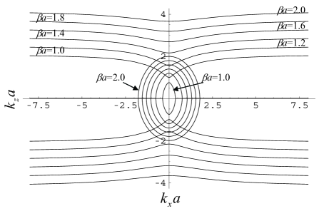
Figure 5: Plot of $k_{z}$ as a function of $k_{x}a$ for $R=0.05a$ and $k_{y}=0$. Contours $\beta a=1.0,1.2,1.4,1.6,1.8,2.0$ for the TM-modes. The permittivity $\epsilon$ follows a Drude type model (see the text).

In Figs. 4 and 5, $k_{z}$ is plotted as a function of $k_{x}$ for $R=0.05a$ and several different values of the normalized frequency $\beta a$ (the permittivity of the rods follows the same Drude model as before). For convenience we show the results in two different figures. For very long wavelengths $\beta_{c}(\omega)<<\beta_{p}$, and consequently one of the modes is cut-off. The dispersion of the other mode (shown in Fig. 4) becomes increasingly flat as the frequency (and consequently $\beta_{c}$) decreases. Note that from (24) and assuming a Drude type model, $\beta_{c}$ increases monotonically with the frequency.

At some point, as the frequency increases, the TM-mode that was cut-off starts to propagate. In this case, (Fig. 5), for each fixed frequency there are two different contours, i.e. two propagating TM-modes. As the frequency increases even more, $\beta_{c}$ becomes comparable or larger than $\beta_{p}$, and the band structure of one of the TM-modes becomes practically flat, consistently with the fact that the energy propagated by this mode is tightly confined to the vicinity of the ENG rods.

In Figs. 4 and 5 it can also be seen that around $k_{||}\approx 0$ the wave normal contours of one of the modes are to some extent hyperbolic. In fact, using (25) it can be easily checked that one of the modes has dispersion characteristic such that the signs of the coefficients associated with $k_{||}^{2}$ and $k_{z}^{2}$ are symmetric. This property is more important for frequencies such that $\beta_{c}(\omega)\approx\beta_{p}$. Note that if the medium was anisotropic, with no spatial dispersion, and negative permittivity along the $z$-direction the contours would also be hyperbolic. It is well-known that hyperbolic contours may originate negative refraction at an interface.

It is also important to refer that in the limit $\varepsilon\to 1$, the ratio $\beta_{c}(\omega)/\beta_{p}$ becomes infinitely large (see (24)) and consequently $k_{z}/\beta$ is also infinitely large. This means that in these circumstances the localized TM-mode either cannot be excited by an incoming wave, or if it is excited it is killed by losses. Thus, only the other TM-mode, with dispersion $k_{z}^{2}\approx\beta^{2}-k_{||}^{2}$, will propagate. This is consistent with the fact that as $\varepsilon\to 1$ the medium shall have the same properties as free-space.

To conclude this section, we will discuss the scope of application of the permittivity model (16). We remember that the results were derived for thin rods, $R<<a$, and under the assumption that $|k_{\rho,0}|a<<\pi$ and $\beta a<<\pi$. In general the modes that propagate in the long wavelength limit satisfy the previous conditions without problems. However, there is one exception at the problem at hand. In fact, when $\beta_{c}(\omega)>>\beta_{p}$ the radial constant $k_{\rho,0}$ becomes complex imaginary for the TM-mode associated with the surface mode (surface plasmon). As discussed in Takahara et al. (1997), when the beam radius is subwavelength the effective index of refraction $n_{eff}=k_{z}/\beta$ becomes very large, and in that case the condition $|k_{\rho,0}|a<<\pi$ may not be observed. This situation affects the accuracy of our model when $\beta_{c}(\omega)>>\beta_{p}$. Indeed, the error in the TM-mode associated with the surface mode becomes non-negligible in this situation. The other TM-mode is still accurately predicted. This result justifies deterioration of the agreement in Fig. 3, as the frequency (and consequently, for the Drude Model, also $\beta_{c}$) increases.

Fortunately, it is easy to solve this problem. In fact, when $\beta_{c}(\omega)>>\beta_{p}$ the dispersion characteristic of the pertinent TM-mode is essentially the same as the dispersion characteristic of the guided mode supported by a single ENG rod. This dispersion characteristic is determined in Takahara et al. (1997), and is equivalent to the condition $\alpha_{zz}^{-1}=0$, where $\alpha_{zz}^{-1}$ is given by (10). Thus, to summarize our findings, the TM-modes can be accurately calculated using (23), except when $\beta_{c}(\omega)>>\beta_{p}$ which yields less accurate results for the mode with higher $k_{z}$. In this case the corresponding TM-mode is dispersionless, and follows the same characteristic as the guided mode supported by a single dielectric rod.

V The Reflection Problem with rods parallel to the interfaces

To further validate the proposed permittivity model, we will study the reflection of electromagnetic waves by a rod medium slab with finite thickness. We will suppose that the rods are parallel to the interface (see Fig. 6). The slab consists of $N_{L}$ layers of rods. The structure is periodic in $y$ and $z$, and the dielectric rods stand in free-space. The interfaces $x=x^{\prime}_{L}$ and $x=x^{\prime}_{R}=x^{\prime}_{L}+N_{L}a$ are represented by the dashed lines (since the rods stand in air the definition of the interfaces is a bit ambiguous; this will be discussed below with more detail). The rods in the leftmost layer are in the plane $x=x_{0}$.

As discussed in the previous section, when the rods are parallel to the interface, equation (22) has only one solution for $k_{x}^{2}$. For simplicity, we will restrict our attention to the case in which either $k_{z}=0$ (Fig. 6a) or $k_{y}=0$ (Fig. 6b). For these particular geometries, an incident plane wave polarized as depicted in Fig. 6 can only excite the TM-mode inside the rod medium. As is well-known Collin (1990), in the general case where $k_{y}$ and $k_{z}$ are simultaneously different from zero, both the TM- and TE-modes are excited (the medium is birefringent). Apart from the more heavy notation, the general case poses no additional difficulties.

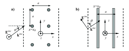
Figure 6: A plane wave illuminates a slab of the rod medium ($N_{L}=2$). The rods are parallel to the plane $x=0$. a) $k_{z}=0$. b) $k_{y}=0$.

Using (29), (21), and (22) and matching the tangential components of the electric and magnetic fields at the interfaces, we find that the reflection coefficient referred to the plane $x=x^{\prime}_{L}$ is given by:

$$\rho=\frac{{\tanh\left({\gamma_{m}d}\right)\left({\gamma_{0}^{2}-\gamma_{m}^{2}}\right)}}{{2\gamma_{0}\gamma_{m}+\tanh\left({\gamma_{m}d}\right)\left({\gamma_{0}^{2}+\gamma_{m}^{2}}\right)}}$$ (26)

$$\rho=\frac{{\tanh\left({\gamma_{m}d}\right)\left({\varepsilon^{2}\gamma_{0}^{2}-\gamma_{m}^{2}}\right)}}{{2\varepsilon\gamma_{0}\gamma_{m}+\tanh\left({\gamma_{m}d}\right)\left({\varepsilon^{2}\gamma_{0}^{2}+\gamma_{m}^{2}}\right)}}$$ (27)

where $d=N_{L}a$ is the thickness of the slab, $\gamma_{m}=j\,k_{x,rod}$, $\gamma_{0}=\sqrt{k_{y}^{2}+k_{z}^{2}-\beta{}^{2}}$, and (26) corresponds to Fig. 6a) with $k_{z}=0$, and (27) corresponds to Fig. 6b) with $k_{y}=0$.

Next, in order to demonstrate the accuracy of the theoretical results, the analytical model is tested against full wave data computed with the periodic moment method (MoM) Wu (1995). In the first example we consider that $R=0.05a$, and $\epsilon=-30.0$ at $\beta a=1.0$ (for simplicity, losses are neglected). A plane wave polarized as depicted in Fig. 6a illuminates 5 layers of rods ($N_{L}=5$). The amplitude of the reflection coefficient is depicted in Fig. 7 as a function of $k_{y}a$. Note that the angle of incidence $\varphi$ is such that $\sin\varphi={{k_{y}}\mathord{\left/{\vphantom{{k_{y}}\beta}}\right.\kern-1.2pt}\beta}$. For $k_{y}>\beta$ the incident wave is evanescent. The solid line represents the MoM full wave data. The dashed line represents the results computed using the proposed permittivity model (formula (26)). It is seen that that the agreement between the two sets of data is good. Similar agreement is obtained for the phase of the reflection coefficient and for the transmission coefficient. The previous results also demonstrate that the homogenization model is useful to study not only incident propagating plane waves, but also part of the evanescent spectrum.

Figure 7: Reflection coefficient as a function of the wave vector component parallel to the interface. The slab consists of $N_{L}=5$ layers, and the rods have $R=0.05a$, and $\epsilon=-30$ at $\beta a=1.0$ The solid line represents the full wave MoM data, and the dashed line represents the data obtained using the analytical model.

Figure 8: Reflection coefficient as a function of $k_{y}a$ for $N_{L}=1$ layer, $R=0.05a$, and $\epsilon=-30$ at $\beta a=1.0$. The solid and dashed lines are defined as in Fig. 7.

As noted before, since the rods stand in free-space the position of the interfaces and thickness of the slab are a bit ambiguous. Notice that the thickness of the homogenized slab was taken equal $d=N_{L}a$, apparently with good results. Next, to test if this choice still yields accurate results for very thin slabs, the reflection coefficient is computed for the same structure, except that now the slab has only one layer of rods ($N_{L}=1$). The reflection coefficient is depicted in Fig. 8 and has a peak at $k_{y}a=1.0$, which corresponds to the transition between propagating waves and evanescent waves. As seen, even though the slab is so thin the agreement is still remarkably good. This is a bit a surprising, because for such a thin slabs one would expect that the interface effects and granularity of the artificial medium would prohibit the homogenization of the structure using the bulk medium average fields.

In the next example, we study what happens if the angle of incidence $\varphi$ is kept constant ($\varphi=45[\rm{deg}]$), and the frequency is varied. Now $R=0.01a$, $N_{L}=5$, and the permittivity follows the Drude model $\epsilon=1-\beta_{m}^{2}/\beta^{2}$ with plasma wave number $\beta_{m}a=12.0$ or $\beta_{m}a=80.0$. The calculated results are shown in Fig. 9. For relatively low frequencies the two sets of data agree very well, but as the frequency increases the agreement progressively deteriorates, since the long wavelength limit approximation is no longer valid. Notice that for relatively low frequencies the medium blocks the incident radiation because the rods effectively behave as perfectly conducting wires.

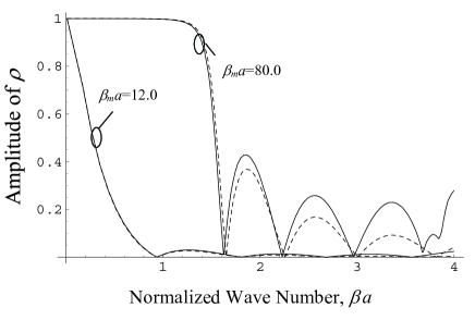
Figure 9: Reflection coefficient as a function of the free-space wave number $\beta a$ for $R=0.01a$, and $N_{L}=5$ layers. The permittivity of the rods follows a Drude-type model (see the text). The solid and dashed lines are defined as in Fig. 7.

Figure 10: Reflection coefficient as a function of $k_{z}a$ for $N_{L}=5$ layer, $R=0.05a$, and $\epsilon=-30$ at $\beta a=1.0$. The solid and dashed lines are defined as in Fig. 7.

So far the wave vector of the incident wave was always perpendicular to the axes of the ENG rods, and so the effects of spatial dispersion were hidden. In the last example, we consider the very different propagation scenario depicted in Fig. 6b. The parameters of the rods are $R=0.05a$, $\epsilon=-30$, and $N_{L}=5$. The reflection coefficient for $\beta a=1.0$ is shown in Fig. 10 as a function of $k_{z}a$. Note that the angle of incidence $\theta$ for propagating waves satisfies $\sin\theta={{k_{z}}\mathord{\left/{\vphantom{{k_{z}}\beta}}\right.\kern-1.2pt}\beta}$. Fig. 10 shows that the agreement between the numerical and analytical results is still quite satisfactory, except near the transition between the propagating waves and the evanescent waves ($k_{z}a\approx 1.0$).

It is important to refer that the configurations studied in this section (rods parallel to the interface) are not appropriate to achieve sub-wavelength imaging. For that application the rods must be perpendicular to the interface, as shown in Fig. 2b. As discussed in section IV, for this geometry three modes are excited in the (homogenized) rod medium, and thus an additional boundary condition is necessary to solve the scattering problem. The same situation occurs in the wire medium Silveirinha (2005). The analysis of this problem is out of the scope of this work and will be presented elsewhere.

VI Conclusion

We studied the electrodynamics of a periodic array of thin ENG rods. Using the polarizability of a single rod and integral equation methods, we derived new nonlocal permittivity model for the artificial medium that accurately describes the propagation of waves in the long wavelength limit. We discussed the effects of spatial dispersion in the context of the reflection problem. It was proved that when the rods are parallel to interface only two modes (TE and TM) can be excited in the artificial medium. However, when the axes of the rods are normal to the interface, two TM-modes, besides the TE- mode, can be excited in the medium, as a manifestation of spatial dispersion. It was demonstrated that the wave normal contours of one of the TM-modes are intrinsically hyperbolic. It was proved that the rod medium supports dispersionless modes that propagate along the axes of the rods, and it was speculated that this important property may allow sub-wavelength imaging of electromagnetic waves at the infrared and optical domains, using the idea proposed in Belov et al. (2005). It was shown that the energy of the dispersionless modes can be loosely bounded to the ENG rods (in this case the wave is essentially transverse electromagnetic), or alternatively tightly confined to a vicinity of the rods. In the latter case, the modes have approximately the same dispersion as the guided surface mode supported by an individual rod. The reflection problem was investigated in detail for the case where rods are parallel to the interfaces. The developed theory was successively tested against full wave data calculated with the MoM.

Appendix A Derivation of the Mixing Formula

In this Appendix we derive the mixing formula (13) used to homogenize the rod medium.

Let us consider a generic electromagnetic Floquet mode $(\bf{E},\bf{H})$, associated with the wave vector ${\bf{k}}=(k_{x},k_{y},k_{z})$ and the wave number $\beta=\omega/c$, i.e. the fields satisfy Maxwell-Equations and $({\bf{E}},{\bf{H}})\exp\left({{j}{\bf{k}}{\bf{.r}}}\right)$ is a periodic function in the lattice. The average electric field is defined as,

$${\bf{E}}_{{\rm{av}}}=\frac{1}{{{\rm{V}}_{{\rm{cell}}}}}\int\limits_{\Omega}{{\bf{E}}\left({\bf{r}}\right)e^{+j\,{\bf{k}}{\bf{.r}}}}d^{3}{\bf{r}}$$ (28)

and ${\bf{H}}_{{\rm{av}}}$ is defined similarly. In the above, $\Omega$ represents the unit cell of the periodic medium. From Maxwell-Equations it can be proved that:

$$-{\bf{k}}\times{\bf{E}}_{{\rm{av}}}+\beta\,\eta_{0}{\bf{H}}_{{\rm{av}}}=0$$ (29)

$$\beta\,\left({{\bf{E}}_{{\rm{av}}}+\frac{{\bf{P}}}{{\varepsilon_{\rm{0}}}}}\right)+{\bf{k}}\times\eta_{0}{\bf{H}}_{{\rm{av}}}=0$$ (30)

where the generalized polarization vector is given by,

$$\frac{{\bf{P}}}{{\varepsilon_{0}}}=\frac{1}{{{\rm{V}}_{{\rm{cell}}}}}\int\limits_{\Omega}{\left({\varepsilon-1}\right){\bf{E}}\,}e^{+j\,{\bf{k}}{\bf{.r}}}d^{3}{\bf{r}}$$ (31)

Straightforward calculations show that these relations imply that:

$${\bf{E}}_{{\rm{av}}}=\frac{{\beta^{2}\overline{\overline{\bf{I}}}-{\bf{kk}}}}{{k^{2}-\beta^{2}}}{\bf{.}}\frac{{\bf{P}}}{{\varepsilon_{0}}}$$ (32)

The above equations are exact and completely general. Next we will apply these results to the rod medium under study. To begin with, we note that since the crystal is invariant to translations along the $z$-direction the fields depend on $z$ as $\exp(-jk_{z}z)$. Using standard Green function methods Collin (1990), it can be proved that the electric field has the following integral representation,

$${\bf{E}}\left({\bf{r}}\right)=\left({\varepsilon-1}\right)\int\limits_{S}{\beta^{2}\overline{\overline{{\bf{G}}}}_{p}\left({\left.{\bf{r}}\right|{\bf{r^{\prime}}}}\right){\bf{.E}}\left({{\bf{r^{\prime}}}}\right)}\,\,d^{2}{\bf{r^{\prime}}}$$ (33)

where the primed and unprimed coordinates represent the source and observation points, respectively, $S=\left\{{\left({x^{\prime},y^{\prime},0}\right):x^{\prime 2}+y^{\prime 2}\leq R^{2}}\right\}$ is the cross-section of the dielectric rod in the unit cell, and the Green function dyadic is defined by,

$$\overline{\overline{{\bf{G}}}}_{p}=\left({\overline{\overline{\bf{I}}}+\frac{1}{{\beta{}^{2}}}\left({\nabla_{||}-jk_{z}{\bf{\hat{u}}}_{z}}\right)\left({\nabla_{||}-jk_{z}{\bf{\hat{u}}}_{z}}\right)}\right)\,\Phi_{p}$$ (34)

In the above, $\Phi_{p}=\Phi_{p}\left({\left.{\bf{r}}\right|{\bf{r^{\prime}}}}\right)$ is the dynamic potential created by a phase-shifted array of line sources,

$$\nabla^{2}\Phi_{p}+\beta^{2}\Phi_{p}=-\sum\limits_{\bf{I}}{\delta\left({{\bf{r_{||}}}-{\bf{r^{\prime}_{||}}}-{\bf{r}}_{\bf{I}}}\right)}e^{-j{\bf{k}}{\bf{.}}\left({{\bf{r}}-{\bf{r^{\prime}}}}\right)}$$ (35)

where $\delta$ is the Dirac function, ${\bf{I}}=(i_{1},i_{2})$ is a double index of integers, ${\bf{r_{I}}}=a(i_{1},i_{2},0)$ is a lattice point, and $r_{||}=(x,y,0)$. Thus $\Phi_{p}$ is intrinsically two-dimensional, depending on $z$ and $z^{\prime}$ as $e^{-jk_{z}\left({z-z^{\prime}}\right)}$. Furthermore, it is obvious that the Green function only depends on the relative position $\bf{r_{||}}-\bf{r^{\prime}_{||}}$. Note that the Green function can be written as a superimposition of the potentials created by the line sources:

$$\Phi_{p}=\sum\limits_{\bf{I}}{\Phi_{0}\left({{\bf{r}}_{||}-{\bf{r^{\prime}}}_{||}-{\bf{r}}_{\bf{I}}}\right)}e^{-j{\bf{k}}{\bf{.r}}_{\bf{I}}}$$ (36)

where $\Phi_{0}=e^{-jk_{z}\left({z-z^{\prime}}\right)}{{H_{0}^{\left(2\right)}\left({k_{\rho,0}\left|{{\bf{r}}_{||}-{\bf{r^{\prime}}}_{||}}\right|}\right)}\mathord{\left/{\vphantom{{H_{0}^{\left(2\right)}\left({\beta\left|{{\bf{r}}_{||}-{\bf{r^{\prime}}}_{||}}\right|}\right)}{4j}}}\right.\kern-1.2pt}{4j}}$ is the potential created by a line source placed at $\bf{r^{\prime}_{||}}$, i.e. the solution of (35) when the summation in the right-hand side is restricted to the index ${\bf{I}}={\bf{0}}$. Physically, (33) establishes that the electric field at some point of space is the superimposition of the fields radiated by all the dielectric rods of the lattice.

The Green potential can also be written as a Fourier series since it is a (pseudo) periodic function of the wave vector:

$$\Phi_{p}\left({\left.{\bf{r}}\right|{\bf{r^{\prime}}}}\right)=\frac{1}{{{\rm{A}}_{{\rm{cell}}}}}\sum\limits_{\bf{J}}{\frac{{e^{-j{\bf{k}}_{\bf{J}}{\bf{.}}\left({{\bf{r}}-{\bf{r^{\prime}}}}\right)}}}{{{\bf{k}}_{\bf{J}}{\bf{.k}}_{\bf{J}}-\beta^{2}}}}$$ (37)

where ${\rm{A}}_{\rm{cell}}=a^{2}$, ${\bf{J}}=(j_{1},j_{2})$ is a double index of integers, ${\bf{k}}_{\bf{J}}={\bf{k}}+{\kern 1.0pt}\,{\bf{k}}_{\bf{J}}^{0}$, and ${\bf{k}}_{\bf{J}}^{0}={{2\pi}\mathord{\left/{\vphantom{{2\pi}a}}\right.\kern-1.2pt}a}\left({j_{1},j_{2},0}\right)$.

Now that the necessary theoretical formalism was introduced, we are ready to study the homogenization problem in the rod medium. To begin with, we note that from (36) and (37) the Green potential is singular in the spatial domain, i.e. when $\bf{r_{||}}-\bf{r^{\prime}_{||}}\approx 0$ (source region), as well as in the spectral domain, i.e. when ${\bf{k}}{\bf{.k}}\approx\beta^{2}$ (long wavelength limit). Since the integral (33) is defined over the source region and we want to study the electromagnetic modes that propagate in the long wavelength limit, it is convenient to single out the terms that make the Green function singular and decompose it as follows:

$$\Phi_{p}=\Phi_{0}+\frac{1}{{{\rm{A}}_{{\rm{cell}}}}}\frac{{e^{-j{\bf{k}}{\bf{.}}\left({{\bf{r}}-{\bf{r^{\prime}}}}\right)}}}{{{\bf{k}}{\bf{.k}}-\beta^{2}}}+\Phi_{reg}$$ (38)

where $\Phi_{reg}$, which is defined implicitly by the above formula, is a regular function both in the spatial domain (source region $\bf{r_{||}}-\bf{r^{\prime}_{||}}\approx 0$) and in the spectral domain (long wavelength limit). Using this decomposition in (33) we find that:

$${\bf{E}}\left({\bf{r}}\right)= {\bf{E}}_{{\rm{av}}}e^{-j{\bf{k}}{\bf{.r}}}+\left({\varepsilon-1}\right)\int\limits_{S}{\beta^{2}\overline{\overline{{\bf{G}}}}_{0}\left({\left.{\bf{r}}\right|{\bf{r^{\prime}}}}\right){\bf{.E}}}\,\,d^{2}{\bf{r^{\prime}}}$$ (39)

$$+\left({\varepsilon-1}\right)\int\limits_{S}{\beta^{2}\overline{\overline{{\bf{G}}}}_{reg}\left({\left.{\bf{r}}\right|{\bf{r^{\prime}}}}\right){\bf{.E}}}\,\,d^{2}{\bf{r^{\prime}}}$$

where ${\bf{E}}_{{\rm{av}}}$ is the average field in the crystal, and $\overline{\overline{{\bf{G}}}}_{0}$ and $\overline{\overline{{\bf{G}}}}_{reg}$ are defined as $\overline{\overline{{\bf{G}}}}_{p}$, except that the Green potential is replaced by $\Phi_{0}$ and $\Phi_{reg}$, respectively. To obtain the above result we used (32). Next, we use the fact that the ENG rods are assumed to be very thin ($R/a<<1$), and that we want to investigate the electrodynamics of modes that propagate in the long wavelength limit ($|{\bf{k_{||}}}|a<<2\pi$ and $\beta a<<2\pi$). Since the dyadic $\overline{\overline{{\bf{G}}}}_{reg}$ is regular in both the spatial and spectral domains, it is legitim to write (putting $\bf{r_{||}}=\bf{r^{\prime}_{||}}=0$ and ${\bf{k_{||}}}=(k_{x},k_{y},0)=\bf{0}$),

$$\overline{\overline{{\bf{G}}}}_{reg}\left({\left.{\bf{r}}\right|{\bf{r^{\prime}}};{\bf{k}},\beta}\right)\approx\overline{\overline{{\bf{G}}}}_{reg}\left({z|z^{\prime};k_{z},\beta}\right)$$ (40)

being the formula valid in the source region. For convenience, we introduce the following interaction dyadic:

$$\overline{\overline{{\bf{C}}}}_{{\mathop{\rm int}}}=\beta^{2}\overline{\overline{{\bf{G}}}}_{reg}\left({0;k_{z},\beta}\right)$$ (41)

Then, it is clear from (39) that,

$${\bf{E}}\left({\bf{r}}\right)\approx \left({{\bf{E}}_{{\rm{av}}}+\overline{\overline{{\bf{C}}}}_{{\mathop{\rm int}}}.\frac{{{\bf{p}}}}{{\varepsilon_{0}}}}\right)e^{-jk_{z}z}$$ (42)

$$+\left({\varepsilon-1}\right)\int\limits_{S}{\beta^{2}\overline{\overline{{\bf{G}}}}_{0}\left({\left.{\bf{r}}\right|{\bf{r^{\prime}}}}\right){\bf{.E}}}\,\,d^{2}{\bf{r^{\prime}}}$$

provided the observation point $\bf{r}$ is near the source region and $|{\bf{k_{||}}}|a<<2\pi$. In above, we introduced the electric dipole moment (per unit of length), ${\bf{p}}$, of the dielectric rod in the unit cell. Now, the key result is that (42) is formally equivalent to the (integral) equation obtained when a single rod is illuminated by a plane wave with electric field with amplitude ${\bf{E}}^{{\rm{inc}}}=\left({{\bf{E}}_{{\rm{av}}}+\overline{\overline{{\bf{C}}}}_{{\mathop{\rm int}}}.\frac{{{\bf{p}}}}{{\varepsilon_{0}}}}\right)$ and the same wave vector component $k_{z}$ along the $z$-direction. In other words, when the rod in the unit cell stands alone in free-space and is illuminated with the above defined plane wave, the total electric field also satisfies (to a first approximation) (42) in the source region. But this remarkable result implies that:

$$\frac{{\bf{p}}}{{\varepsilon_{0}}}=\overline{\overline{{\bf{\alpha}}}}_{e}{\bf{.}}\left({{\bf{E}}_{{\rm{av}}}+\overline{\overline{{\bf{C}}}}_{{\mathop{\rm int}}}{\bf{.}}\frac{{\bf{p}}}{{\varepsilon_{0}}}}\right)$$ (43)

where $\overline{\overline{{\bf{\alpha}}}}_{e}$ is the electric polarizability tensor for a single rod. The term inside brackets in the right-hand side can be regarded as the local field that polarizes a single rod embedded in the dielectric crystal. Within the thin rod condition and for long wavelengths, the above solution is exact.

We are now ready to calculate the effective permittivity dyadic. Since the (macroscopic) electric displacement vector $\bf{D}$ is given by ${\bf{D}}=\varepsilon_{0}{\bf{E}}_{{\rm{av}}}+{{\bf{p}}\mathord{\left/{\vphantom{{\bf{p}}{{\rm{A}}_{{\rm{cell}}}}}}\right.\kern-1.2pt}{{\rm{A}}_{{\rm{cell}}}}}$, and the effective permittivity tensor must guarantee that ${\bf{D}}=\varepsilon_{0}\overline{\overline{\varepsilon}}{\bf{.E}}_{{\rm{av}}}$, we conclude that the effective permittivity of the rod medium is given by the mixing formula (13). Note that (13) is completely general and is valid independently of the specific geometry of the transverse section of the rod.

At this point it is appropriate to compare (13) with the classic homogenization approach. It is striking that (13) reminds Clausius-Mossotti formula Collin (1990); Sihvola (1999). Indeed, if we could identify the interaction dyadic $\overline{\overline{{\bf{C}}}}_{{\mathop{\rm int}}}$ with ${1\mathord{\left/{\vphantom{1{2{\rm{A}}_{{\rm{cell}}}}}}\right.\kern-1.2pt}{2{\rm{A}}_{{\rm{cell}}}}}$ the formulas would be the same (note also that the rods are arranged in a square lattice). In Appendix B we calculate the interaction dyadic in closed-form using the static limit approximation. Equation (47) shows that the interaction dyadic is different from ${1\mathord{\left/{\vphantom{1{2{\rm{A}}_{{\rm{cell}}}}}}\right.\kern-1.2pt}{2{\rm{A}}_{{\rm{cell}}}}}$ only along the $z$-direction. This important result shows that Clausius-Mossotti formula is not valid for media with cylindrical inclusions. More specifically it fails to predict the effective permittivity along the direction in which the crystal is uniform. This is an indirect manifestation of spatial dispersion.

We also mention that the interaction dyadic defined by (41) is not equivalent to the dynamic interaction constant defined in other works (see for example Belov and Simovski (2005)). Indeed, in our definition we extracted the singularities in both the spatial and spectral domains, while other works usually only extract the singularity in the spatial domain. It is clear from our previous analysis that it is the singularity in the spectral domain that indirectly defines the relation between the local field that polarizes the rod and the average field.

Appendix B Calculation of the interaction dyadic

Here we calculate the interaction dyadic defined by (41). It can be written as:

$$\overline{\overline{{\bf{C}}}}_{{\mathop{\rm int}}}=\left({\beta^{2}\overline{\overline{\bf{I}}}+\left({\nabla_{||}-jk_{z}{\bf{\hat{u}}}_{z}}\right)\left({\nabla_{||}-jk_{z}{\bf{\hat{u}}}_{z}}\right)}\right)\Phi_{reg}$$ (44)

where the right-hand side of the expression is evaluated at $\bf{r}=\bf{r^{\prime}}=0$ and $\bf{k_{||}}=0$. From (35) and (38) it is clear that:

$$\nabla^{2}\Phi_{reg}+\beta^{2}\Phi_{reg}=$$

$$\left(\frac{1}{{{\rm{A}}_{{\rm{cell}}}}}-\sum\limits_{{\bf{I}}\neq{\bf{0}}}{\delta\left({{\bf{r_{||}}}-{\bf{r^{\prime}_{||}}}-{\bf{r}}_{\bf{I}}}\right)}\right)e^{-j{\bf{k}}{\bf{.}}\left({{\bf{r}}-{\bf{r^{\prime}}}}\right)}$$ (45)

Putting $\bf{r}=\bf{r^{\prime}}=0$ and $\bf{k}=0$ in the above equation, and letting $\beta$ approach zero (static limit), we find that:

$$\left.{\nabla^{2}\Phi_{reg}\left({{\bf{r}}={\bf{r^{\prime}}}=0;{\bf{k}}={\bf{0}}}\right)}\right|_{\beta=0}=\frac{1}{{{\rm{A}}_{{\rm{cell}}}}}$$ (46)

Moreover, because of the symmetry of the square lattice it is evident that if $\bf{r}=\bf{r^{\prime}}=0$ and $\bf{k}=0$ the following relations hold, $\frac{{\partial^{2}\Phi_{reg}}}{{\partial x_{i}\partial x_{j}}}=0$ if $i\neq j$, $\frac{{\partial^{2}\Phi_{reg}}}{{\partial z^{2}}}=0$, and $\frac{{\partial^{2}\Phi_{reg}}}{{\partial x^{2}}}=\frac{{\partial^{2}\Phi_{reg}}}{{\partial y^{2}}}$. So using (46), we conclude that in the static limit ($\bf{k}=0$ and $\beta=0$) the interaction dyadic is given by:

$$\overline{\overline{{\bf{C}}}}_{{\mathop{\rm int}}}=\frac{1}{{2{\rm{A}}_{{\rm{cell}}}}}\left({\overline{\overline{\bf{I}}}-{\bf{\hat{u}}}_{z}{\bf{\hat{u}}}_{z}}\right)$$ (47)

The above result is consistent in the $xoy$ plane with the (two dimensional version of the) Clausius-Mossotti formula. However, along the $z$-direction, maybe a bit surprisingly, the interaction constant vanishes in the static limit. Next, we will estimate ${C_{{\mathop{\rm int}},zz}}$ in the dynamic case. From (44), we have that:

$$C_{{\mathop{\rm int}},zz}=\left({\beta^{2}-k_{z}^{2}}\right)\Phi_{reg}$$ (48)

Using (36) and (38), and putting $\bf{r}=\bf{r^{\prime}}=0$ and $\bf{k}_{||}=0$, we obtain that:

$$C_{{\mathop{\rm int}},zz}=\left({\beta^{2}-k_{z}^{2}}\right)\sum\limits_{{\bf{I}}\neq 0}{\frac{1}{{4j}}H_{0}^{\left(2\right)}\left({k_{\rho,0}\left|{{\bf{r}}_{\bf{I}}}\right|}\right)}+\frac{1}{{{\rm{A}}_{{\rm{cell}}}}}$$ (49)

The series in the right-hand side was evaluated in Belov et al. (2002). Using the results of Belov et al. (2002), and assuming that $k_{\rho,0}a<<\pi$, we obtain:

$$C_{{\mathop{\rm int}},zz}\approx k_{\rho,0}^{2}\left({\frac{j}{4}+\frac{1}{{2\pi}}\ln\left({\frac{{k_{\rho,0}a}}{{4\pi}}}\right)+\frac{C}{{2\pi}}+}\right.$$ (50)

$$\left.{+\frac{1}{{12}}+\sum\limits_{n=1}^{\infty}{\frac{1}{{\pi\left|n\right|}}\frac{1}{{e^{2\pi\left|n\right|}-1}}}}\right)$$

where $C$ is the Euler constant.

References

- Veselago (1968) V. Veselago, Sov. Phys. Usp. 10, 509 (1968).
- Shelby et al. (2001) R. A. Shelby, D. R. Smith, and S. Schultz, Science 77, 292 (2001).
- Pendry (2000) J. Pendry, Phys. Rev. Lett. 85, 3966 (2000).
- Belov et al. (2005) P. A. Belov, C. R. Simovski, and P. Ikonen, Phys. Rev. B. 71, 193105 (2005).
- Belov et al. (2006) P. A. Belov, Y. Hao, and S. Sudhakaran, Phys. Rev. B. 73, 033108 (2006).
- Poulton et al. (2004) C. Poulton, S. Guenneau, and A. B. Movchan, Phys. Rev. B 69, 195112 (2004).
- Pokrovsky (2004) A. L. Pokrovsky, Phys. Rev. B 69, 195108 (2004).
- Pokrovsky and Efros (2002a) A. L. Pokrovsky and A. L. Efros, Phys. Rev. Lett. 89, 093901 (2002a).
- Pokrovsky and Efros (2002b) A. L. Pokrovsky and A. L. Efros, Phys. Rev. B 65, 045110 (2002b).
- Belov et al. (2003) P. Belov, R. Marques, S. Maslovski, I. Nefedov, M. Silveirinha, C. Simovski, and S. Tretyakov, Phys. Rev. B 67, 113103 (2003).
- Silveirinha and Fernandes (2005a) M. Silveirinha and C. A. Fernandes, IEEE Trans. on Microwave Theory and Tech. 53, 1418 (2005a).
- Simovski and Belov (2004) C. R. Simovski and P. A. Belov, Phys. Rev. E 70, 046616 (2004).
- Silveirinha and Fernandes (2005b) M. Silveirinha and C. A. Fernandes, IEEE Trans. on Antennas and Propagat. 53, 59 (2005b).
- Belov et al. (2002) P. Belov, S. Tretyakov, and A. Viitanen, J. Electromagn. Waves Applic. 16, 1153 (2002).
- Silveirinha (2005) M. Silveirinha, to appear in IEEE Trans. Antennas. Propagat. (June 2006) (arxiv: cond-mat/0509612) (2005).
- Sihvola (1999) A. Sihvola, Electromagnetic mixing formulas and applications (IEE Electromagnetic Waves Series 47, 1999).
- Takahara et al. (1997) J. Takahara, S. Yamagishi, H. Taki, A. Morimoto, and T. Kobayashi, Optics Letters 22, 475 (1997).
- Collin (1990) R. Collin, Field Theory of Guided Waves (IEEE Press, Piscataway, NJ, 1990).
- Wu (1995) T. Wu, Frequency-selective surface and grid array (Wiley, NY, 1995).
- Belov and Simovski (2005) P. A. Belov and C. R. Simovski, Phys. Rev. E 72, 026615 (2005).