Relaxation, dephasing, and quantum control of electron spins in double quantum dots

Abstract

Recent experiments have demonstrated quantum manipulation of two-electron spin states in double quantum dots using electrically controlled exchange interactions. Here, we present a detailed theory for electron spin dynamics in two-electron double dot systems that was used to guide those experiments and analyze the results. Specifically, we analyze both spin and charge relaxation and dephasing mechanisms that are relevant to experiments, and discuss practical approaches for quantum control of two-electron systems. We show that both charge and spin dephasing play important roles in the dynamics of the two-spin system, but neither represents a fundamental limit for electrical control of spin degrees of freedom in semiconductor quantum bits.

Electron spins in quantum dots represent a promising system for studying mesoscopic physics, developing elements for spintronics Awschalom et al. (2002); awschalom07 , and creating building blocks for quantum information processing Loss and DiVincenzo (1998); Imamoglu et al. (1999); Taylor et al. (2005a); hansonrmp06 . In the field of quantum information, confined electron spins have been suggested as a potential realization of a quantum bit, due to their potential for long coherence times Khaetskii and Nazarov (2000, 2001); Golovach et al. (2004). However, the deleterious effects of hyperfine coupling to lattice nuclear spins Schulten and Wolynes (1978); Burkard et al. (1999); Merkulov et al. (2002); Khaetskii et al. (2002); Erlingsson and Nazarov (2002); de Sousa and Sarma (2003); Coish and Loss (2004); Yao et al. (2005); Deng and Hu (2005), as found in experiments Bracker et al. (2005); Johnson et al. (2005); Koppens et al. (2005); Petta et al. (2005a); koppens06 , can severely limit the phase coherence of electron spins. Thus, it is important to understand dynamics of electron spin coupled to nuclei and to develop corresponding quantum control techniques to mitigate this coupling.

Recent experiments by our group explored coherent spin manipulation of electron spins to observe and suppress the hyperfine interaction Johnson et al. (2005); Petta et al. (2005a); laird06 . In this paper, we present a detailed theory describing coherent properties of coupled electrons in double quantum dots that was used to guide those experiments and analyze the results. The theory includes hyperfine interactions, external magnetic field, exchange terms, and charge interactions.

Our approach relies upon an approximation based on the separation of time scales between electron spin dynamics and nuclear spin dynamics. In particular, the time scales governing nuclear spin evolution are slower than most relevant electron spin processes. This allows us to treat the nuclear environment using a type of adiabatic approximation, the quasi-static approximation (QSA) Schulten and Wolynes (1978); Merkulov et al. (2002). In this model, the nuclear configuration is fixed over electron spin precession times, but changes randomly on the time scale over which data points in an experiment might be averaged (current experiments acquire a single data point on $\sim$ 100 ms timescales). We also consider the first corrections to this approximation, where experimentally relevant.

In what follows, we start by reviewing the theory of hyperfine interactions in single and double quantum dots, focusing on electrostatic control of electron spin-electron spin interactions. We then consider the role of charge dephasing and charge-based decay in experiments involving so-called spin blockade, in which a simultaneous spin flip and charge transition is required for electrons to tunnel from one dot to another Johnson et al. (2005). Consistent with the experiments, we find that blockade is reduced near zero magnetic field over a range set by the average magnitude of the random Overhauser (nuclear) field. We then consider the effect of fast control of the local electrostatic potentials of double quantum dots, and show how this may be used to perform exchange gates Loss and DiVincenzo (1998); Burkard et al. (1999); Schliemann et al. (2001), and to prepare and measure two-spin entangled states Taylor et al. (2005b); Petta et al. (2005a). Various limitations to the preparation, manipulation, and measurement techniques, due to nuclear spins, phonons, and classical noise sources, are considered.

Theories that explicitly include quantum mechanical state and evolution effects of the nuclear spins both within and beyond the QSA have been considered by several authors (Refs. Burkard et al., 1999; Khaetskii et al., 2002; Coish and Loss, 2004; Shenvi et al., 2005; Coish and Loss, 2005; Witzel et al., 2005; Yao et al., 2005; Deng and Hu, 2005). Dephasing, decoherence, and gating error in double quantum dots have also been investigated previously Coish and Loss (2005); Hu and Sarma (2005); Klauser et al. (2005); the present work develops the theory behind quantum control techniques used in experiments, connecting the previous general theoretical treatments to specific experimental observations. The paper is organized as follows. Interactions of a single electron in a single quantum dot, including hyperfine terms, are reviewed in section I. The quasi-static regime is defined and investigated, and dephasing of electron spins by hyperfine interactions in the quasi-static regime is detailed. This provides a basis for extending the results to double quantum dot systems. We then develop a theory describing the two-electron spin states of a double quantum dot including the response of the system to changes in external gate voltages, and the role of inelastic charge transitions Brandes and Kramer (1999); Fujisawa et al. (2001); Brandes and Vorrath (2002). This is combined with the theory of spin interactions in a single dot to produce a theory describing the dynamics of the low energy states, including spin terms, of the double dot system in two experimental regimes. One is near the charge transition between the two dots, where the charge state of two electrons in one dot is nearly degenerate with the state with one electron in each dot. The other is the far-detuned regime, where the two dots are balanced such that the states with two electrons in either dot are much higher in energy.

In the remaining sections, we investigate situations related to the experiments. First we consider spin blockade near the charge transition, as investigated in Ref. Johnson et al., 2005, considering effects due to difference in dot sizes and expanding upon several earlier, informal ideas. We then analyze approaches to probing dephasing and exchange interactions, showing how errors effect fast gate control approaches for preparation and measurement of two-electron spin states, as well as controlled exchange interactions and probing of nuclear-spin-related dephasing, as investigated in Ref. Petta et al., 2005a. Finally, we consider limitations to exchange gates and quantum memory of logical qubits encoded in double dot systems Taylor et al. (2005b, a).

I Hyperfine interactions in a double quantum dot: a review

We begin by reviewing the basic physics of hyperfine interactions for electron spins in single GaAs quantum dots. This section reviews the established theory for single quantum dots Schulten and Wolynes (1978); Merkulov et al. (2002); Khaetskii et al. (2002); de Sousa and Das Sarma (2003) and considers dynamical corrections to the model of Refs. Schulten and Wolynes, 1978; Merkulov et al., 2002. This model will be used in subsequent sections for the double-dot case. Additional terms, such as spin-orbit coupling, are neglected. Theory Khaetskii and Nazarov (2000, 2001); Golovach et al. (2004) and experiment Hanson et al. (2003); Kroutvar et al. (2004); Johnson et al. (2005) have demonstrated that spin-orbit related terms lead to dephasing and relaxation on time scales of milliseconds, whereas we will focus on interaction times on the order of nanoseconds to microseconds.

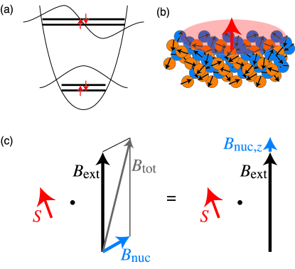
Figure 1: (a) A schematic potential and energy level diagram for a single quantum dot in which one electron is confined to the low energy spectrum of a three dimensional potential. Only the ground and first-excited states, each a Kramer’s doublet, are shown. (b) The lowest orbital state has a spin-1/2 electron interacting with the lattice nuclear spins. (c) Effective magnetic field due to both external field and the nuclear field. When the external field is large, the transverse components of the nuclear field are neglected in a rotating wave approximation.

I.1 Electron spin Hamiltonian for a single quantum dot

The Hamiltonian for the Kramer’s doublet of the ground orbital state of the quantum dot (denoted by the spin-1/2 vector $\hat{\vec{S}}$) including hyperfine contact interactions with lattice nuclei (spins $\hat{\vec{I}}^{\beta,j}$) is Paget et al. (1977); Merkulov et al. (2002)

$$H=\hbar\gamma_{e}\vec{B}_{\rm ext}\cdot\hat{\vec{S}}+\hbar\gamma_{e}\sum_{\beta,j}b_{\beta}\alpha_{j,\beta}\hat{\vec{S}}\cdot\hat{\vec{I}}^{\beta,j}$$ (1)

where $\gamma_{e}=g^{*}\mu_{B}/\hbar$ is the gyromagnetic ratio for electron spin $\hat{\vec{S}}$; sums are over nuclear species ($\beta$) and unit cells ($j$). Correspondingly, $b_{\beta}$ is the effective hyperfine field due to species $\beta$ within a unit cell, with $b_{\rm{}^{75}As}=-1.84$ T, $b_{\rm{}^{69}Ga}=-1.52$ T, and $b_{\rm{}^{71}Ga}=-1.95$ T for GaAs Paget et al. (1977). The coefficient $\alpha_{j,\beta}=v_{0}|\psi(\vec{r}_{j,\beta})|^{2}$ is the probability of the electron being at unit cell $j$ (with nuclear spin species $\beta$), $v_{0}$ is the volume of the unit cell (2 nuclei), and $\psi(r)$ is the envelope wavefunction of the localized electron.

It is convenient to rewrite the Hamiltonian using a collective operator for the nuclear spins, $\hat{\vec{B}}_{\rm nuc}=\sum_{\beta}b_{\beta}\sum_{j}\alpha_{j,\beta}\hat{\vec{I}}^{\beta,j}$. This operator allows us to write the Hamiltonian as an electron spin interacting with an external magnetic field, $\vec{B}_{\rm ext}$, and an intrinsic field, $\hat{\vec{B}}_{\rm nuc}$:

$$H_{\rm eff}=\hbar\gamma_{e}(\vec{B}_{\rm ext}+\hat{\vec{B}}_{\rm nuc})\cdot\hat{\vec{S}}~{}.$$ (2)

Several characteristic values Paget et al. (1977); Merkulov et al. (2002) for this interaction are noted in Table 1. The maximum nuclear field value (all spins fully polarized with value $I=3/2$) is $h_{0}=\sum_{\beta}b_{\beta}(x_{\beta}I^{\beta})\sum_{k}\alpha_{k}$, where we have separated out the relative population of nuclear species, $x_{\rm{}^{75}As}=1$, $x_{\rm{}^{69}Ga}=0.6$, and $x_{\rm{}^{71}Ga}=0.4$ for GaAs, removing the $\beta$ dependence from the $\alpha_{k,\beta}$. This gives $b_{0}=5.3$ T. Second, when the nuclear spins may be described by a density matrix $\rho=\hat{1}/(2I+1)^{N}$ (infinite temperature approximation for $N$ nuclei), the root-mean-square (rms) strength of the field is

$$B_{\rm nuc} = \sqrt{\langle|\hat{\vec{B}}_{\rm nuc}|^{2}\rangle/3}=\sqrt{\sum_{\beta,k}b_{\beta}^{2}\alpha_{k,\beta}^{2}\langle|\hat{\vec{I}}^{\beta,k}|^{2}\rangle/3}$$ (3)

$$= \sqrt{(\sum_{\beta}x_{\beta}b_{\beta}^{2})I(I+1)v_{0}/3\int d^{3}r\ |\psi(r)|^{4}}$$ (4)

$$= h_{1}/\sqrt{N}\ .$$ (5)

where we have replaced $\sum_{j}v_{0}$ with $\int d^{3}r$. The characteristic strength parameter is $h_{1}=\sqrt{2I(I+1)/3\sum_{\beta}x_{\beta}b_{\beta}^{2}}=4.0$ T for GaAs, and $N$ is defined as the number of nuclei with which the electron has significant overlap, i.e., $N=2/[\int d^{3}r\ |\psi(r)|^{4}v_{0}]$. These numerical values are specific for GaAs quantum dots. Dots in other materials with non-zero nuclear spin may be described by similar parameters: a maximum field strength parameter $h_{0}$ and a rms field strength parameter, $B_{\rm nuc}=h_{1}/\sqrt{N}$.

I.2 The quasi-static approximation for nuclear spins

By writing the Hamiltonian (Eq. 2) with nuclei as an effective magnetic field, we have implicitly indicated that the field may be considered on a similar footing to the external magnetic field. In other words, the operator $\hat{\vec{B}}_{\rm nuc}$ may be replaced by a random, classical vector $\vec{B}_{\rm nuc}$, and observables may be calculated by averaging over the distribution of classical values. The distribution in the large $N$ limit is

$$P(\vec{B})=\frac{1}{(2\pi B_{\rm nuc}^{2})^{3/2}}\exp(-(\vec{B}\cdot\vec{B})/2B_{\rm nuc}^{2})\ .$$ (6)

This is the quasi-static approximation (QSA) used in Refs. Schulten and Wolynes, 1978; Merkulov et al., 2002: we assume that over time scales corresponding to electron spin evolution, the nuclear terms do not vary.

In terms of dephasing, we cite the results of Ref. Merkulov et al., 2002. At zero external magnetic field in the Heisenberg picture, the electron spin $\hat{\vec{S}}$ evolves to:

$$\langle\hat{\vec{S}}(t)\rangle_{\rm nuc}=\frac{\hat{\vec{S}}(0)}{3}(1+2(1-(\gamma_{e}B_{\rm nuc}t)^{2})e^{-(\gamma_{e}B_{\rm nuc}t)^{2}}).$$ (7)

On the other hand, at large external magnetic fields, $\hat{S}_{z}$ is conserved, but transverse spin components (e.g., $\hat{S}_{x}$) decay as:

$$\langle\hat{S}_{x}\rangle_{\rm nuc}=\frac{\hat{S}_{x}}{2}(1+e^{-\frac{1}{2}(\gamma_{e}B_{\rm nuc}t)^{2}})\ .$$ (8)

A time-ensemble-averaged dephasing time due to nuclei in a single dot at large external magnetic field (e.g., dot $i$) is

$$T_{2,i}^{*}=\frac{1}{\gamma_{e}B_{{\rm nuc},i}}\ .$$ (9)

This definition is appropriate when considering the decay of coherence of a single electron in a single quantum dot.

Generalizing to all field values, for times longer than $T_{2}^{*}$,

$$\hat{\vec{S}}(t\gg T_{2}^{*})=\langle(\hat{\vec{S}}(t=0)\cdot\vec{n})\vec{n}\rangle_{\rm nuc}$$ (10)

is the average electron spin value, averaged over a time $\tau=2\pi/\omega$.

Type	Time	Energy	Magnetic field	Typical value
Charge
Charging energy		$E_{c}$		5 meV
Orbital level spacing		$\hbar\omega_{0}$		1 meV
Single dot two-electron exchange near $B_{\rm ext}=0$		$\mathcal{J}$		300 $\mu$eV
Double-dot tunnel coupling		$T_{c}$		10 $\mu$eV
Double-dot inelastic tunneling		$\Gamma(\epsilon)$		0.01–100 neV
Electron spin
Larmor precession	$t_{L}$	$\hbar\gamma_{e}B_{\rm ext}$	$B_{\rm ext}$	0–200 $\mu$eV
Fully polarized overhauser shift		$AI$	$h_{0}$	130 $\mu$eV
(Random) overhauser shift	$T_{2}^{*}$	$\hbar\gamma_{e}B_{\rm nuc}$	$B_{\rm nuc}=\frac{h_{1}}{\sqrt{N}}$	0.1–1 $\mu$eV
Nuclear spin species $\beta$
Larmor precession	$t_{nL,\beta}$	$\hbar\gamma_{\beta}B_{\rm ext}$	$B_{\rm ext}$	0–100 neV
Knight shift	$t_{K,\beta}$	$\hbar\gamma_{e}B_{\rm nuc}\lambda_{\beta,j}\approx\frac{\hbar\gamma_{e}B_{\rm nuc}}{\sqrt{N}}$	$\frac{\gamma_{e}B_{\rm nuc}}{\gamma_{\beta}\sqrt{N}}$	0.1–10 neV
Dipole-dipole interaction (nearest neighbor)	$t_{dd}$	$\frac{(\hbar\gamma_{\beta})^{2}}{v_{0}}$	$\frac{\hbar\gamma_{\beta}}{v_{0}}$	0.01 neV

Table 1: Time, energy, and magnetic field scales for electron and nuclear spins in a single and double quantum dots, from fast to slow.

At low magnetic fields, the QSA is valid up to the single electron spin-nuclear spin interaction time ($O(\hbar N/A)$), which is of order microseconds Merkulov et al. (2002). In contrast, at large external fields, the regime of validity for the QSA is extended. Terms non-commuting with the Zeeman interaction may be eliminated (secular approximation or rotating wave approximation), yielding an effective Hamiltonian

$$H_{\rm eff}=\hbar\gamma_{e}(B_{\rm ext}+B_{{\rm nuc}}^{z})\hat{S}_{z}\ .$$ (11)

The $z$ axis is set to be parallel to the external magnetic field. Corrections to the QSA have a simple interpretation in the large field limit. As the Zeeman energy suppresses spin-flip processes, we can create an effective Hamiltonian expanded in powers of $1/B_{\rm ext}$ using a Schrieffer-Wolf transformation. In the interaction picture, we write the corrections to $H_{\rm eff}$ by setting $B_{{\rm nuc}}^{z}=B_{z}+\delta\hat{B}_{z}(t)$, where $B_{z}$ is the QSA term, and $\delta\hat{B}_{z}(t)$ are fluctuations beyond the QSA. When the number of nuclei $N$ is large and fluctuations small, we approximate $\delta\hat{B}_{z}$ by its fourier transformed correlation function:

$$\langle\delta\hat{B}_{z}(t+\tau)\delta\hat{B}_{z}(t)\rangle=\int d\omega\ S(\omega)e^{i\omega\tau}$$ (12)

where $S(\omega)$ has a high frequency cutoff $\gamma\ll\gamma_{e}B_{\rm nuc}$. The form of $S(\omega)$ depends on the detailed parameters of the nuclear spin Hamiltonian and the nuclear spin-nuclear spin interactions, and in general requires a many-body treatment. A variety of approaches have been used to successfully estimate these corrections Shenvi et al. (2005); Coish and Loss (2005); Witzel et al. (2005); Yao et al. (2005); Deng and Hu (2005); witzel06 . Any approach with an expansion in inverse powers of the external field is compatible with our assumption of $S(\omega)$, provided that the number of nuclear spins is sufficiently large that Gaussian statistics may emerge. In contrast, the validity of the QSA in the low-field regime remains unproven, though recent simulations Al-Hassanieh et al. (2006) suggest it may break-down before $\hbar\sqrt{N}/A$ timescales.

I.3 Hyperfine interactions in a double quantum dot

We consider standard extensions to the single electron theoretical model to describe the case of two electrons in adjacent, coupled quantum dots, by considering only charge-related couplings, then including spin couplings. The relevant states are separated electron states, in which one electron is in each quantum dot, and doubly-occupied states, with two electrons in one of the two dots.

The doubly-occupied states are assumed to be singlets (appropriate for small perpendicular magnetic field) Burkard et al. (1999). The higher excited states that are doubly-occupied are triplets with a large energy gap $\mathcal{J}$. This singlet–triplet energy gap for doubly-occupied states facilitates elimination of the spin interactions and the doubly-occupied triplet states. Furthermore, by controlling the relative potential $\epsilon$ of the two quantum dots using electrostatic potentials applied by external gates, the ground state can be changed from one of the doubly-occupied states to one of the separated electron states (far-detuned regime on the other side of the charge transition) vanderwiel . Electrostatic control of the double dot Hamiltonian will be analyzed in more detail in sections II–IV.

Formally, we eliminate all but one of the doubly-occupied states following the prescription of Ref. Coish and Loss, 2005. We include the doubly-occupied state (0,2)S, where ($n_{l},n_{r}$) denotes number of electrons in left, right dots respectively, and S denotes a singlet of electron spin, in addition to the singlet and triplet manifolds of the (1,1) subspace. For notational convenience, we set $\epsilon=0$ to occur at the avoided crossing between (1,1) and (0,2) in Fig. 2. There is an avoided crossing at $\epsilon=0$ for the spin singlet manifold due to quantum mechanical tunneling $T_{c}$ between the two quantum dots, while the spin triplet manifold is unaffected. The Hamiltonian for the states $\left|(0,2)S\right>$, $\left|(1,1)S\right>$ can be written as

$$H_{11-02}=\left(\begin{array}[]{cc}-\epsilon&T_{c}\\ T_{c}^{*}&0\\ \end{array}\right)\ .$$ (13)

As the tunneling coefficient and external magnetic field are assumed constant, we will choose $T_{c}$ to be real by an appropriate choice of gauge

For a slowly varying or time-independent Hamiltonian, the eigenstates of Eq. 13 are given by

$$\left|\tilde{S}\right> = \cos\theta\left|S\right>+\sin\theta\left|(0,2)S\right>$$ (14)

$$\left|\tilde{G}\right> = -\sin\theta\left|S\right>+\cos\theta\left|(0,2)S\right>\ .$$ (15)

We introduce the tilde states as the adiabatic states, with $\left|\tilde{G}\right>$ the higher energy state. The adiabatic angle is $\theta=\arctan(\frac{2T_{c}}{\epsilon-\sqrt{4|T_{c}|^{2}+\epsilon^{2}}})$, and the energies of the two states are

$$E_{\tilde{S}} = -\frac{T_{c}}{2}\tan(\theta)$$ (16)

$$E_{\tilde{G}} = \frac{T_{c}}{2}\tan(\pi/2-\theta)\ .$$ (17)

When $\epsilon\ll-|T_{c}|$, $\theta\rightarrow 0$, the eigenstates become $\left|\tilde{S}\right>\rightarrow\left|S\right>,\left|\tilde{G}\right>\rightarrow\left|(0,2)S\right>$. For $\epsilon\gg|T_{c}|$, $\theta\rightarrow\pi/2$, and the eigenstates are switched, with $\left|\tilde{S}\right>\rightarrow\left|(0,2)S\right>$ and $\left|\tilde{G}\right>\rightarrow\left|S\right>$. As will be discussed later, controllably changing $\epsilon$ allows for adiabatic passage between the near degenerate spin states $\left|S\right>,\left|T_{m}\right>$ (far detuned regime) to past the charge transition, with $\left|(0,2)S\right>$ as the ground state ($\epsilon\gg|T_{c}|$). This adiabatic passage can be used for singlet generation, singlet detection, and implementation of exchange gates Petta et al. (2005a).

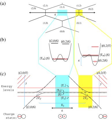
Figure 2: (a) Charge stability diagram for a double dot system. Double dot occupation is denoted by ($n_{l},n_{r}$). The detuning is parameterized by $\epsilon$, and the far-detuned regime (light blue) and charge transition (yellow) are shown. (b) Schematic of the double well potentials along one axis ($x$) with tight confinement in the other two axes (i.e., $y$ and $z$). In the far-detuned regime, the (1,1) charge states are the ground state, while in the charge transition regime, (0,2) can be the ground state. Triplet states are indicated in red, while electron charges are indicated in orange. (c) Energy level structure of the double dot system as a function of detuning. From left to right the lowest energy charge state as a function of $\epsilon$ is (2,0), (1,1), and (0,2). The detuning at the middle of the graph corresponds to $\epsilon=-E_{c}/2$, where $E_{c}$ is the charging energy of a single dot. The three (1,1) triplet states (shown in red) are split by Zeeman energy.

We now add spin couplings to the double dot system, including both Zeeman interactions and hyperfine contact coupling. Two effective Hamiltonians, one for $\epsilon\ll-|T_{c}|$ and one for $\epsilon\sim 0$ are developed. Our approach is similar to that of Ref. Coish and Loss, 2005, and we include it here for completeness. The spin interactions in a double quantum dot for the states $\left|T_{m}\right>,\left|\tilde{S}\right>$ may be written for $\epsilon\ll-|T_{c}|$ as

$$H_{\rm hf,tot}=H_{\rm hf,eff}^{l}+H_{\rm hf,eff}^{r}-J(\epsilon)|S\rangle\!\langle S|$$ (18)

where $l$ and $r$ refer to left and right dot, respectively, the nuclear fields are determined by the ground orbital state envelope wavefunctions of the single dot Hamiltonians (see Fig. 3), and $J(\epsilon)=-E_{\tilde{S}}(\epsilon)$.

Figure 3: A double quantum dot in the (1,1) configuration. (a) Schematic of the two-electron wavefunction in the far-detuned regime interacting with lattice nuclear spins. (b) Electron spins in the left and right dots interacting with their respective effective nuclear fields in the quasi-static approximation.

Reordering terms simplifies the expression:

$$H_{\rm hf,tot}=\hbar\gamma_{e}[\vec{B}\cdot(\hat{\vec{S}}^{l}+\hat{\vec{S}}^{r})+\vec{dB}\cdot(\hat{\vec{S}}^{l}-\hat{\vec{S}}^{r})]-J(\epsilon)|S\rangle\!\langle S|$$ (19)

with an average field $\vec{B}=\vec{B}_{\rm ext}+\frac{\vec{B}_{\rm nuc,l}+\vec{B}_{\rm nuc,r}}{2}$ and difference field $\vec{dB}=(\vec{B}_{\rm nuc,l}-\vec{B}_{\rm nuc,r})/2$. The form of Eqn. 19 indicates that terms with $\vec{B}$ and $J(\epsilon)$ are diagonal in total spin and spin projection along $\vec{B}$, creating a natural set of singlet and triplet states. However, the term with $\vec{dB}$ breaks total spin symmetry, and couples the singlet to the triplet states.

We can now write Eqn. 19 in matrix form in the basis $\{\left|T_{+}\right>,\left|T_{0}\right>,\left|T_{-}\right>,\left|S\right>\}$,

$$H=\hbar\gamma_{e}\left(\begin{matrix}B_{z}&0&0&\frac{dB_{x}-idB_{y}}{\sqrt{2}}\\ 0&0&0&-dB_{z}\\ 0&0&-B_{z}&\frac{-dB_{x}-idB_{y}}{\sqrt{2}}\\ \frac{dB_{x}+idB_{y}}{\sqrt{2}}&-dB_{z}&\frac{-dB_{x}+idB_{y}}{\sqrt{2}}&-J(\epsilon)/\gamma_{e}\end{matrix}\right)$$ (20)

The corresponding level structure is given in Fig. 4a. We have implicitly assumed the QSA in writing this Hamiltonian by defining the axis of spin up and down as $\vec{B}$, which is a sum of the external field and the average nuclear field. If the nuclear field fluctuates, those terms can contribute by coupling different triplet states together.

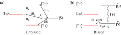
Figure 4: (a) Levels in the far-detuned regime including all couplings of Eqn. 20. (b) Levels near the charge transition; the $\left|T_{+}\right>\leftrightarrow\left|\tilde{S}\right>$ is near resonance, with the coupling between $\left|T_{+}\right>$ and $\left|\tilde{S}\right>$ indicated, as per Eqn. 22.

With no external magnetic field, all states couple to the singlet, and solving the dynamics requires diagonalizing the 4-by-4 matrix of Eqn. 20. However, at finite magnetic field, a large Zeeman splitting (which sets $B_{z}\gg B_{\rm nuc}$) allows us to separate the system. The far-detuned regime only has transitions between the $m_{s}=0$ states; in this basis ($\{\left|T_{0}\right>,\left|S\right>\}$), the matrix becomes

$$H_{m_{s}=0}=\hbar\gamma_{e}\left(\begin{matrix}0&-dB_{z}\\ -dB_{z}&-J(\epsilon)/\gamma_{e}\end{matrix}\right).$$ (21)

This two-level system has appropriately straightforward dynamics, and we investigate it in some detail below.

Near the charge transition and at finite magnetic field, another coupling can occur, this time between $\left|T_{+}\right>$ and $\left|\tilde{S}\right>$. This resonance corresponds to the adiabatic singlet $\left|\tilde{S}\right>$ having an exchange energy $J(\epsilon)$ close to the Zeeman-split triplet’s Zeeman energy, $E_{z}=\hbar\gamma_{e}B_{z}$. We note that external magnetic field for GaAs will be negative in this context (due to the negative electron $g$-factor = -0.44). Written in the basis $\{\left|T_{+}\right>,\left|\tilde{S}\right>\}$, the Hamiltonian is

$$H_{\rm flip-flop}=\hbar\gamma_{e}\left(\begin{matrix}B_{z}&\frac{dB_{x}-idB_{y}}{\sqrt{2}}\cos\theta\\ \frac{dB_{x}+idB_{y}}{\sqrt{2}}\cos\theta&-J(\epsilon)/\gamma_{e}\end{matrix}\right).$$ (22)

We have subscripted Eqn. 22 with “flip-flop” indicating that flips between $\left|\tilde{S}\right>$ and $\left|T_{+}\right>$ result in the flipping of a nuclear spin, which can be seen by identifying $dB_{+}=dB_{x}+idB_{y}=(\hat{B}_{\rm nuc,l,+}-\hat{B}_{\rm nuc,r,+})/2$.

Because the $\tilde{S}$–$T_{+}$ resonance leads to spin flips and eventual polarization of the nuclear field, the QSA will not be valid if appreciable change of field occurs, and the overall dynamics may go beyond the approximation. This has been examined experimentally Ono and Tarucha (2004); Koppens et al. (2005) and theoretically Taylor et al. (2003); Erlingsson et al. (2003); ramon06 for some specific cases. While the discussion to follow mentions this resonance, it will focus on the zero field mixing of Eqn. 19 and the far-detuned regime’s finite field mixing of Eqn. 21. We remark that Eqns. 21 and 22 have been previously derived outside of the QSA Coish and Loss (2005).

We have now established that in the far-detuned regime, the relevant spin interactions are limited to dynamics within the singlet-triplet subspace and determined by the Hamiltonian in Eqn. 21. Similarly, near the charge transition a resonance between $\left|S\right>$ and $\left|T_{+}\right>$ may be observed; as this resonance allows for nuclear spin polarization, it may only be partially described by the QSA, and we do not consider its dynamics in detail. However, we note that in the absence of nuclear spin polarization the resonance occurs when the Zeeman splitting of the external field equals the exchange energy, $J(\epsilon)$. Thus, if the Zeeman energy is known, measuring the position of the splitting gives a map between external parameters and the actual exchange energy.

II Nuclear-spin-mediated relaxation in double dots

In this section we consider the case in which the ground state of the system is $\left|(0,2)S\right>$ and the low-lying excited states are the (1,1) states, $\{\left|S\right>,\left|T_{m}\right>\}$. This situation occurs in dc transport when the system is in the spin blockade regime, where transitions from $\left|T_{m}\right>$ to $\left|(0,2)S\right>$ are suppressed because they require both a spin and charge transition. Previous theoretical work for two electron systems has focused on triplet and singlet decay of two-electron states in a single quantum dot erlingsson01 ; in contrast, the present analysis deals with a double quantum dot system where the electrons can be well separated. Contrary to more general spin blockade calculationsjouravlev05 and experiments, the present work is focused entirely on the rate limiting step of blockade: the spin flip followed by charge transition within the double quantum dot. Several groupsHanson et al. (2003); Elzerman et al. (2004); Kroutvar et al. (2004) have studied spin relaxation between Zeeman split spin states at high magnetic field ($B>$4 T). The measured relaxation rates were found to scale as $B^{4}$, consistent with a spin-orbit mediated spin relaxation processGolovach et al. (2004). Similarly, single dot measurements of triplet-singlet relaxation when $\mathcal{J}\gg\gamma_{e}B_{\rm nuc}$ (i.e., when the effect of nuclei is small) indicate long lifetimes, likely limited by similar spin-orbit mediated mechanisms or cotunneling to the leadsFujisawa et al. (2001); meunier06 . On the other hand, at low field and small exchange, when the splitting between spin states becomes comparable to $B_{\rm nuc}$, the hyperfine interaction dramatically increases the spin relaxation rate. Recent experiments have measured spin relaxation between nearly degenerate singlet and triplet spin states in this regime Johnson et al. (2005); hanson05 . Experimental techniques are discussed in Ref. Petta et al. (2005b), and a full analysis of the field and energy dependence of the relaxation rate is discussed in Ref. Johnson et al. (2005). We only briefly outline the salient features of experiment, focusing instead on developing a more rigorous basis for the theory of previous, published work.

Experiments are performed near the two-electron regime with very weak tunnel coupling so that $T_{c}$ is slower than the pulse rise times ($T_{c}\ll 1\mu$eV). Pulsed-gate techniques are used to change the charge occupancy from (0,1) to (1,1) to (0,2) and back to (0,1). In the (1,1) charge configuration with weak interdot tunnel coupling the $\left|S\right>$ and $\left|T_{m}\right>$ states are nearly degenerate. Shifting the gates from (0,1) to (1,1) creates a mixture of all four states, $\left|S\right>,\left|T_{m=-1,0,1}\right>$ by loading an electron from a nearby Fermi sea. Then, the system is rapidly (non-adiabatic with respect to tunnel coupling $T_{c}$) shifted to the (0,2) regime, with $\left|(0,2)S\right>$ as the ground state. In this rapid shift procedure, the singlet $\left|S\right>$ does not adiabatically follow to the doubly-occupied singlet $\left|(0,2)S\right>$, but instead follows the Zener branch of the avoided crossing and stays in $\left|S\right>$, as is illustrated in Fig. 5.

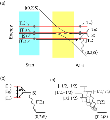
Figure 5: (a) Energy level structure as a function of detuning. Coupling to a Fermi sea with $k_{b}T\gg\gamma_{e}|B_{\rm ext}|$ leads to equal filling of all four low energy states in the far-detuned regime (labelled start). Then $\epsilon$ is changed rapidly with respect to the tunnel coupling, leading to all four spin states still in the (1,1) charge configuration. The time spent waiting in this configuration results in slow decay of the metastable (1,1) states to the $\left|(0,2)S\right>$ state. (b) Nuclear spins couple between the eigenstates of exchange, and slow inelastic decay at a rate $\Gamma$ proceeds from $\left|S\right>$ to $\left|(0,2)S\right>$. (c) The same process, but for the eigenstates of the double dot Hamiltonian. The $m_{s}=0$ states are equal superpositions of $\left|S\right>$ and decay rapidly to $\left|(0,2)S\right>$, while the $|m_{s}|=1$ states are only weakly mixed at large magnetic field with the $\left|S\right>$, resulting in slow decay to $\left|(0,2)S\right>$.

Past the charge transition, when the adiabatic basis $\left|\tilde{S}\right>,\left|\tilde{G}\right>$ is an appropriate representation of the system, it is possible for the system to experience inelastic decay from the excited state $\left|\tilde{G}\right>$ to the ground state $\left|\tilde{S}\right>$ via charge coupling, e.g., to phonons. The energy gap for $\epsilon\gg|T_{c}|$ is $E_{\tilde{G}}-E_{\tilde{S}}=\sqrt{\epsilon^{2}+4|T_{c}|^{2}}\approx\epsilon$. Inelastic decay near a charge transition in a double quantum dot has been investigated in great detail Fujisawa et al. (1998); Brandes and Kramer (1999); Brandes and Vorrath (2002), and we do not seek to reproduce those results. Instead, we note that the decay from the excited state $\left|\tilde{G}\right>$ to the ground state $\left|\tilde{S}\right>$ is well described by a smoothly varying, energy-dependent decay rate $\Gamma_{ph}(\epsilon)$. Incoherent population of $\left|\tilde{G}\right>$ by absorption of a thermal phonon is suppressed as long as $2T_{c}>k_{b}T$, which is satisfied for $T_{c}=0.01$ meV and $T=100$ mK.

Finally, we can combine the coherent spin precession due to interaction with nuclear spins with the charge-based decay and dephasing mechanisms to investigate relaxation of $\left|T_{m}\right>$ states to the state $\left|\tilde{S}\right>$. Of particular interest is the regime past the charge transition, $\epsilon\gg T_{c}$, where $\left|\tilde{G}\right>\approx\left|S\right>$ becomes nearly degenerate with $\left|T_{0}\right>$, as was studied in the experiment of Ref. Johnson et al., 2005. An effective five-level system is formed with the levels $\{\left|T_{+}\right>,\left|T_{0}\right>,\left|T_{-}\right>,\left|S\right>\}$ described by the spin Hamiltonian of Eqn. 20, while inelastic decay from $\left|S\right>$ to $\left|(0,2)S\right>$ (the fifth level) is possible at a rate $\Gamma(\epsilon)$, as shown in Fig. 5b.

To analyze this process, we start with the Louivillian superoperator that describes inelastic tunneling:

$$\dot{\rho} = i[\rho,H/\hbar]+\Gamma(\epsilon)/2\Big{[}|S\rangle\!\langle S|\rho+\rho|S\rangle\!\langle S|$$ (23)

$$\ \ -2|(0,2)S\rangle\!\langle S|\rho|S\rangle\!\langle(0,2)S|\Big{]}$$

where

$$H=\hbar\gamma_{e}[\vec{B}^{l}\cdot\hat{\vec{S}}^{l}+\vec{B}^{r}\cdot\hat{\vec{S}}^{r}]_{(1,1)}-\hbar\epsilon|(0,2)S\rangle\!\langle(0,2)S|\ .$$ (24)

$l$ and $r$ indicate left and right spins for the (1,1) charge space. Assuming the nuclear field is quasi-static (QSA), we can diagonalize $H$. The eigenstates are the ground state, $\left|(0,2)S\right>$, and (1,1) states with spin aligned and anti-aligned with the local magnetic fields, $\vec{B}^{l,r}=\vec{B}_{\rm ext}+\vec{B}_{\rm nuc}^{l,r}$. We write these eigenstates as $\left|s,s^{\prime}\right>=\left|s\right>_{l}\otimes\left|s\right>_{r}$, where $s,s^{\prime}=\pm 1/2$ are the eigenvalues of the spin projection on the fields of the $l$ and $r$ dots, respectively. The eigenvalue for $\left|(0,2)S\right>$ is $E_{G}=-\epsilon$ and the other four eigenstates $\left|s,s^{\prime}\right>$ have energy

$$E_{s,s^{\prime}}=s\gamma_{e}|B^{l}|+s^{\prime}\gamma_{e}|B^{r}|\ .$$ (25)

In considering decay from the energy eigenstates of the nuclear field, $\left|s,s^{\prime}\right>$ to $\left|(0,2)S\right>$, we eliminate rapidly varying phase terms, e.g., $\left|1/2,-1/2\right>\left<-1/2,1/2\right|$. This is appropriate provided that the inelastic decay mechanism, $\Gamma(\epsilon)$, is slow in comparison to the electrons’ Larmor precession in the nuclear field $B_{\rm nuc}$. In this limit, each state $\left|s,s^{\prime}\right>$ decays to $\left|(0,2)S\right>$ with a rate given by $\Gamma(\epsilon)|\left\langle s,s^{\prime}\vphantom{(0,2)S}\right.\left|\vphantom{s,s^{\prime}}(0,2)S\right\rangle|^{2}$, as indicated in Fig. 5c. A detailed analysis is given in appendix A. For convenience, we write $c_{s,s^{\prime}}=\left\langle s,s^{\prime}\vphantom{(0,2)S}\right.\left|\vphantom{s,s^{\prime}}(0,2)S\right\rangle$.

Starting with a mixed state of the (1,1) subspace (as in Ref. Johnson et al., 2005), we can find analytical expressions for the time evolution of the density matrix of an initial form $\rho(t=0)=\sum_{s,s^{\prime}}|s,s^{\prime}\rangle\!\langle s,s^{\prime}|/4$. This initial state corresponds to a mixture of the four (1,1) spin states. The charge measurement distinguishes only between (1,1) states and $\left|(0,2)S\right>$; accordingly, we evaluate the evolution of the projector for the (1,1) subspace $P_{11}=\sum_{s,s^{\prime}}|s,s^{\prime}\rangle\!\langle s,s^{\prime}|$. In particular,

$$P_{11}(t)=e^{-\Gamma(\epsilon)|c_{++}|^{2}t}/2+e^{-\Gamma(\epsilon)|c_{+-}|^{2}t}/2$$ (26)

.

Finally, we must average over possible initial nuclear spin configurations to find the measured signal. This means evaluating $\langle P_{11}(t)\rangle_{\rm nuc}$, a difficult task in general. However,

$$\langle P_{11}(t)\rangle_{\rm nuc}\approx e^{-\Gamma(\epsilon)\langle|c_{++}|^{2}\rangle_{\rm nuc}t}/2+e^{-\Gamma(\epsilon)\langle|c_{+-}|^{2}\rangle_{\rm nuc}t}/2\ .$$ (27)

In this approximation, we replace the average of the exponents with the average values for the coefficients $|c_{++}|^{2},|c_{+-}|^{2}$. The validity of this approximation can be checked with numerical integration, and for the range of parameters presented here the approximation holds to better than 1%.

The mean values of the coefficients $|c_{++}|^{2},|c_{+-}|^{2}$ are in turn straightforward to calculate approximately (as done in Ref. Johnson et al., 2005, supplemental information ), giving

$$\Gamma_{+-}=\Gamma(\epsilon)\langle|c_{+-}|^{2}\rangle_{\rm nuc} = \frac{\Gamma(\epsilon)}{4}(1+I_{l}I_{r})$$ (28)

$$\Gamma_{++}=\Gamma(\epsilon)\langle|c_{++}|^{2}\rangle_{\rm nuc} = \frac{\Gamma(\epsilon)}{4}(1-I_{l}I_{r})$$ (29)

with

$$I_{l}=\frac{1}{\sqrt{[1+3(\frac{B_{{\rm nuc},l}}{B_{\rm ext}})^{2}]}}$$ (30)

and similarly for $I_{r}$. We plot the product $I_{l}I_{r}$, found in both Eqns. 28-29, as a function of external magnetic field for increasing difference in dot sizes in Fig. 6. This indicates that the effective decay rates are largely independent of the ratio of dot sizes, relying only on the average effective nuclear field, $B_{\rm nuc}=(B_{{\rm nuc},l}+B_{{\rm nuc},r})/2$.

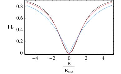
Figure 6: The product $I_{l}I_{r}$ as a function of external magnetic field $B$ in units of average nuclear field, $B_{\rm nuc}=(B_{{\rm nuc},l}+B_{{\rm nuc},l})/2$. Several ratios of dot nuclear fields, $r=B_{{\rm nuc},l}/B_{{\rm nuc},r}$ are considered: $r=1$ (black), $r=1/3$ (red) and $r=0$ (blue). Cusp behavior near zero field is found in the limit of highly inhomogeneous dot field strengths.

We find that past the charge transition with $\epsilon\gg|T_{c}|$ the states $\left|S\right>$ and $\left|T_{0}\right>$ decay to $\left|(0,2)S\right>$ with a lifetime $\Gamma_{+-}^{-1}$, while the two $|m_{s}|=1$ triplet states have a lifetime $\Gamma_{++}^{-1}$. At finite magnetic field, $\Gamma_{+-}\gg\Gamma_{++}$, and we can call the states of the $|m_{s}|=1$ subspace “metastable”. The metastability allows for charge-based measurement to distinguish between $\{\left|S\right>,\left|T_{0}\right>\}$ and $\left|T_{\pm}\right>$ subspaces: by using a nearby charge sensor, the decay of $\left|S\right>,\left|T_{0}\right>$ may be detected long before $\left|T_{\pm}\right>$ has finite probability of decay in the weak tunneling limit. This indicates that, while at zero field decay of the (1,1) states to the state $\left|(0,2)S\right>$ is governed by a single exponential, a double-exponential behavior appears as $B>B_{\rm nuc}$ is satisfied, in direct confirmation of the results of Ref. Johnson et al., 2005.

Contrary to expectation, the blockade is contributed to solely by the $|m_{s}|=1$ triplet states. In particular, spin blockade is charge transport at finite bias through, for example, the charge states $(0,1)\rightarrow(1,1)\rightarrow(0,2)$. For biases between left and right leads that are less than $\mathcal{J}$ only the four (1,1) spin states and the state $\left|(0,2)S\right>$ are necessary for understanding the process. An electron (of arbitrary spin) loads from the left lead, creating with equal probability any of the states $\left|s,s^{\prime}\right>$. This then tunnels with a rate $\Gamma_{+-}$ or $\Gamma_{++}$ to the state $\left|(0,2)S\right>$, after which the extra electron on the right tunnels into the leads, and the cycle repeats anew. The average current through the device is dominated by the slowest rate, which in the absence of cotunneling, is $\Gamma_{++}$. In other words, loading into a spin-aligned state $\left|s,s\right>$ prevents further charge transport until it decays, with rate $\Gamma_{++}$, or is replaced from the leads by a cotunneling process.

The measurements by Johnson et al. demonstrate that the transition probability from (1,1) to $\left|(0,2)S\right>$ depends strongly on both magnetic field and detuning Johnson et al. (2005). Our theoretical model, which accounts for hyperfine mixing coupled with inelastic decay agrees well with experimental results for timescales less than 1 ms. The discrepancy between experiment and theory for longer times suggests that other spin relaxation processes may become important above 1 ms (spin-orbit).

III Quantum control of two electron spin states

We now analyze how time-dependent control of gate parameters (e.g., $\epsilon$) may be used to control electron spin in double quantum dots. Of particular interest are methods for probing the hyperfine interaction more directly than in the previous section. The new techniques we use are primarily rapid adiabatic passage and slow adiabatic passage. Rapid adiabatic passage (RAP) can prepare a separated, two-spin entangled state ($\left|S\right>$ in the far-detuned regime), and when reversed, allows a projective measurement that distinguishes the state $\left|S\right>$ from the triplet states, $\left|T_{m}\right>$. A similar technique used at large external magnetic field, slow adiabatic passage (SAP), instead prepares and measures eigenstates of the nuclear field, $\left|s,-s\right>$. We connect these techniques with the experiments in Ref. Petta et al., 2005a and estimate their performance.

III.1 Spin-to-charge conversion for preparation and measurement

Adiabatic passage from $\epsilon\ll-T_{c}$ to $\epsilon\gg T_{c}$ maps the far-detuned regime states $\left|S\right>,\left|T_{m}\right>$ to the states past the charge transition $\left|(0,2)S\right>,\left|T_{m}\right>$, allowing for a charge measurement to distinguish between these results Taylor et al. (2005b); Petta et al. (2005a). In the quantum optics literature, when adiabatic transfer of states is fast with respect to the relevant dephasing (nuclear spin-induced mixing, in our case), it is called “rapid adiabatic passage” (RAP) and we adopt that terminology here.

When the change of detuning, $\epsilon$, is adiabatic with respect to tunnel coupling, $T_{c}$, but much faster than $\gamma_{e}B_{\rm nuc}$ (the hyperfine coupling), the adiabatic passage is independent of the nuclear dynamics. For example, starting past the charge transition with the state $\left|(0,2)S\right>(=\left|\tilde{S}\right>)$ and $\epsilon\gg T_{c}$ and using RAP to the far-detuned regime causes adiabatic following to the state $\left|S\right>$. This prepares a separated, entangled spin state. The procedure is shown in Fig. 7a.

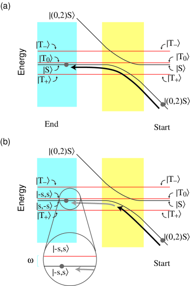
Figure 7: (a) Rapid-adiabatic passage: starting in the state $\left|(0,2)S\right>$, the detuning is changed from $\epsilon\gg T_{c}$ to $\epsilon\ll-T_{c}$, fast with respect to the nuclear energy scale, $\gamma_{e}B_{\rm nuc}$. (b) Slow adiabatic passage: as above, but once the system is past the $S-T_{+}$ degeneracy point, the change of $\epsilon$ is made slow with respect to the nuclear energy scale. The zoomed-in section shows the current nuclear energy splitting ($\hat{\omega}$) and the nuclear field eigenstates, $\left|s,-s\right>$ and $\left|-s,s\right>$. Both procedures may be reversed to transfer either $\left|S\right>$ (RAP) or $\left|s,-s\right>$ (SAP) to $\left|(0,2)S\right>$ while keeping the other states within the (1,1) charge configuration, allowing for charge-based measurement of the system.

The reverse procedure may be used to convert the singlet state to the charge state (0,2) while the triplet remains in (1,1). Then, charge measurement distinguishes singlet versus triplet. Specifically, if we start with some superposition in the far-detuned regime, $\left|\psi\right>=c_{S}\left|S\right>+\sum_{m}c_{m}\left|T_{m}\right>$ where $c_{S},c_{m}$ are quantum amplitudes, after RAP past the charge transition, with $\epsilon\gg T_{c}$, the state is $\left|\psi^{\prime}\right>=c_{S}e^{i\phi}\left|(0,2)S\right>+\sum_{m}c_{m}\left|T_{m}\right>$, where $\phi$ is the adiabatic phase accumulated. Recalling that $\left|(0,2)S\right>$ is in the (0,2) charge subspace, while $\left|T_{m}\right>$ states are in the (1,1) subspace, a nearby electrometer may distinguish between these two results, performing a projective measurement that leaves the $\left|T_{m}\right>$ subspace untouched. Furthermore this measurement is independent of the adiabatic phase.

In contrast, if the change of $\epsilon$ is slow with respect to nuclei, adiabatic passage follows to eigenstates of the hyperfine interaction. For simplicity, we assume that RAP is used between the charge transition to just past the $S-T_{+}$ resonance of Eqn. 22, such that we may neglect transfer between the $S$ and $T_{+}$ states (see also Fig. 8b. This requires an external magnetic field $|B_{\rm ext}|\gg B_{\rm nuc}$. Continuing from this ($\epsilon<-T_{c}$) point to the far-detuned regime, $\epsilon$ is changed slowly with respect to $\hbar\gamma_{e}B_{\rm nuc}$. Accordingly, adiabatic passage proceeds into eigenstates of the nuclear field, $\left|s,-s\right>$, as shown in Fig. 7b. These are the product spin states, with one spin up and the other down with respect to magnetic field. This technique may be called slow adiabatic passage (SAP).

Rapid adiabatic passage maps $\left|S\right>\leftrightarrow e^{i\phi}\left|(0,2)S\right>,\left|T_{m}\right>\leftrightarrow\left|T_{m}\right>$, leaving the triplet states unperturbed. For SAP, the mapping is

$$\left\{\begin{array}[]{ccc}\left|(0,2)S\right>&\leftrightarrow&e^{i\phi}\left|s,-s\right>\\ \left|T_{0}\right>&\leftrightarrow&e^{i\phi^{\prime}}\left|-s,s\right>\\ \left|T_{\pm 1}\right>&\leftrightarrow&\left|T_{\pm 1}\right>\end{array}\right.$$ (31)

It is always the current, lowest energy eigenstate of the nuclear field that $\left|(0,2)S\right>$ maps to. That is, we choose $s$ such that $E_{s,-s}<E_{-s,s}$, with $E_{s,-s}=s\gamma_{e}(B^{l}_{{\rm nuc},z}-B^{r}_{{\rm nuc},z})$, (see Section II, Eqn. 25, evaluated at large external magnetic field). We remark that SAP allows for deterministic preparation and measurement of states rotated $\pi/2$ with respect to $\left|S\right>,\left|T_{0}\right>$ without direct knowledge of which states they correspond to for each realization.

We now examine the adiabaticity condition for slow adiabatic passage. In SAP, $\epsilon$ is changed at a constant rate to approach the far-detuned regime (point S). Using the approximate relation $J(\epsilon)=4T_{c}^{2}/\epsilon$, the adiabaticity condition is $\hbar\dot{J}\ll(\hbar\omega)^{2}$. Neglecting factors of order unity, this can be rewritten $\hbar\dot{\epsilon}\frac{T_{c}^{2}}{\epsilon^{2}}\ll(\hbar\omega)^{2}$.

As a specific case, we consider $T_{c}\simeq 5\ \mu$eV, and $\epsilon\in[50,550]\ \mu$eV. The required time to make the 500 $\mu$eV change, $\tau$, gives $\hbar\dot{\epsilon}=\frac{\hbar}{\tau}500\ \mu$eV, and roughly, $\hbar\dot{\epsilon}\frac{T_{c}^{2}}{\epsilon^{2}}=\frac{\hbar}{\tau}\times 50$ neV. In units of time, $\hbar^{2}(\tau\times 13\ {\rm ns})$. For $\tau=1000$ ns, the adiabaticity requirement is that the current value of $1/|\omega|\lesssim 3\times\sqrt{1000\times 13}\ {\rm ns}=\ 300$ ns. For the nuclear fields in lateral quantum dots such as those of Ref. Johnson et al., 2005 (each dot with a $T_{2}^{*}=10$ ns), the probability of $1/|\omega|>300$ ns is

$$P(|\omega|<3\ \mu{\rm s}^{-1})=2\int_{0}^{3\ \mu{\rm s}^{-1}}d\nu\ \frac{e^{-(\nu T_{2}^{*})^{2}}}{\sqrt{\pi(T_{2}^{*})^{-2}}}$$ (32)

This gives an error probability of 3% for 300 ns rise time, that is, every 1 in 30 experimental runs, the nuclear gradient will be too small for the adiabatic filling of $\left|\pm\right>$ to occur.

We can ask the effect of finite, residual exchange energy $J_{{\rm res}}$ at the S point. Finite $J$ leads to filling of a superposition of $\left|s,-s\right>$ and $\left|-s,s\right>$:

$$\cos(\phi)\left|s,-s\right>-\sin(\phi)\left|-s,s\right>~{},$$ (33)

where the value of $s$ is, as above, determined by the current value of $\omega$ and $\phi=\arctan[J_{{\rm res}}/(\sqrt{J_{{\rm res}}^{2}+\omega^{2}}+|\omega|)]$ is the adiabatic angle. The resulting loss of contrast will be $\sin^{2}(\phi)\simeq(J/2\omega)^{2}$. For residual $J_{{\rm res}}\sim 0.1\ \Omega$, the error is less than 1%. For $J_{{\rm res}}\sim 0.25\ \Omega$ the error is order 2%. The role of residual nuclear fields during the exchange gate is evaluated elsewhere Taylor and Lukin (2005).

III.2 Probing the nuclear field and exchange interactions with adiabatic passage

We now consider how adiabatic passage can be used to probe the dephasing and exchange energy of a spin-singlet state. This relates directly to a critical question in quantum information science: how long can two electron spins remain entangled when the electrons are spatially separated on a GaAs chip. In our model, variations in the local nuclear environment cause the spatially separated electrons to experience distinct local magnetic fields, and hence precess at different rates, mixing the singlet and triplet states. If many measurements are taken to determine the probability of remaining a singlet, the time-ensemble-averaging leads to an observable dephasing of the singlet state ($T_{2}^{*}$) Petta et al. (2005a).

To evaluate the effects of nuclei on this process, we will calculate the singlet autocorrelation function $A_{S}(t)=|\left\langle S(t)\vphantom{S(0)}\right.\left|\vphantom{S(t)}S(0)\right\rangle|^{2}$ for the far-detuned regime. This autocorrelation function has been evaluated for quantum chemistry Schulten and Wolynes (1978), but not for this specific scenario. We remark that our approach is similar to the single dot case considered in Refs. Merkulov et al., 2002; Khaetskii et al., 2002.

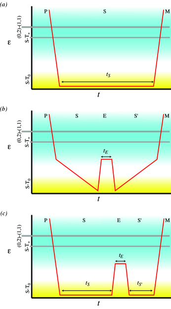
Figure 8: Pulse sequences: detuning parameter $\epsilon$ versus time, for (a) RAP for measurement of the singlet autocorrelation function, (b) SAP for the exchange-gate sequence, and (c) the singlet-triplet echo sequence. Blue is the charge transition region, while yellow is the far-detuned regime. The charge degeneracy point (the crossing from (1,1) to (0,2)) and the degeneracy between $\left|\tilde{S}\right>$ and $\left|T_{+}\right>$ (when $j(\epsilon)=\gamma_{e}|B_{\rm ext}|$) are shown for reference.

We start by evaluating the evolution operation $U(t)$, where the Schrodinger picture $\left|S(t)\right>=U(t)\left|S\right>$. Taking $J\rightarrow 0$ for the far-detuned regime, we solve analytically the equation of motion any spin state of the (1,1) subspace. In particular, we take the Hamiltonian of Eqn. 18 and write it in the form two effective fields, each acting separately on one spin. The evolution operator, $U(t)=\exp(-iHt/\hbar)$ can be factorized as $U(t)=U_{l}(t)\otimes U_{r}(t)$, where

$$U_{i}(t)=\exp(-i\gamma_{e}t[\vec{B}+\vec{B}_{{\rm nuc},i}]\cdot\vec{S}_{i})$$ (34)

is a rotation of spin $i$ about an axis $\vec{n}_{i}=(x_{i},y_{i},z_{i})\propto\vec{B}+\vec{B}_{{\rm nuc},i}$ of angle $t\omega_{i}$ where

$\omega_{i}=\gamma_{e}|\vec{B}+\vec{B}_{{\rm nuc},i}|/2$.

If the system is prepared by RAP in the state $\left|S(t=0)\right>=(\left|\uparrow\downarrow\right>-\left|\downarrow\uparrow\right>)/\sqrt{2}$, and subsequently measured using RAP to distinguish the singlet and triplet subspaces, the measurement probes the state’s autocorrelation function. Starting in a singlet at $t=0$, the probability of remaining a singlet after a time $t$ is given by the autocorrelation function

$$A_{S}(t,B) = |\left\langle S(t)\vphantom{S(t=0)}\right.\left|\vphantom{S(t)}S(t=0)\right\rangle|^{2}$$

$$= |\cos(\omega_{l}t)\cos(\omega_{r}t)+\vec{n}_{l}\cdot\vec{n}_{r}\sin(\omega_{l}t)\sin(\omega_{r}t)|^{2}$$

To obtain the signal in the quasi-static approximation, Eqn. III.2 must be averaged over the different possible nuclear field values. We examine the zero-field and finite-field cases.

When $\vec{B}=0$, the properties of $\vec{n}_{i}$ within the QSA are described by $\langle n_{i,\mu}n_{j,\nu}\rangle=\delta_{ij}\delta_{\mu\nu}/3$. Averaging over nuclei, the signal is

$$A_{S}(t,0) = \langle\cos^{2}(\omega_{l}t)\rangle_{\rm nuc}\langle\cos^{2}(\omega_{r}t)\rangle_{\rm nuc}+$$ (36)

$$\ \ \frac{1}{3}\langle\sin^{2}(\omega_{l}t)\rangle_{\rm nuc}\langle\sin^{2}(\omega_{r}t)\rangle_{\rm nuc}$$

where

$$\langle\cos^{2}(\omega_{i}t)\rangle_{\rm nuc} = \frac{1}{2}[1+e^{-\frac{1}{2}(t/T_{2,i}^{*})^{2}}(1-(t/T_{2,i}^{*})^{2})]~{},$$

$$\langle\sin^{2}(\omega_{i}t)\rangle_{\rm nuc} = \frac{1}{2}[1-e^{-\frac{1}{2}(t/T_{2,i}^{*})^{2}}(1-(t/T_{2,i}^{*})^{2})]~{}.$$

We recall that $T_{2,i}^{*}=(\gamma_{e}B_{{\rm nuc},i})^{-1}$. A distinct difference of this model from other dephasing mechanisms is the order 10% overshoot of the decay at short times, and the asymptoptic approach of $A_{S}(t\gg T_{2}^{*},0)$ to 1/3. A classical master equation would exhibit neither of these features—they are unique identifiers of the quasi-static regime, in which different coherent dynamics are averaged over many realizations. Numerically we find that these qualitative features do not depend on the relative size of the two quantum dots ($B_{{\rm nuc},l}/B_{{\rm nuc},r}$) for variations of up to 50%.

Another regime of interest is when the external field is much larger than the effective nuclear fields ($|\vec{B}|\gg B_{{\rm nuc},i}$). Spin-flip terms are highly suppressed and the system is restricted to two levels, $\left|S\right>$ and the $m_{s}=0$ triplet, $\left|T_{0}\right>=(\left|\uparrow\downarrow\right>+\left|\downarrow\uparrow\right>)/\sqrt{2}$. This is described by the Hamiltonian of Eqn. 21. This effective two-level system’s evolution operator is straightforward to evaluate:

$$A_{S}(t,B\gg B_{\rm nuc})=\langle\cos^{2}(\hat{\omega}t)\rangle=\frac{1}{2}[1+e^{-(t/T_{2,{\rm eff}}^{*})^{2}}]\ .$$ (37)

with $T_{2,{\rm eff}}^{*}=1/\sqrt{\frac{1}{2}[(T_{2,l}^{*})^{-2}+(T_{2,r}^{*})^{-2}]}$. Qualitatively, the decay of the autocorrelation function $A_{S}$ due to the nuclear field is described by Gaussian decay with a timescale $T_{2,{\rm eff}}^{*}$. Similar to the case of zero magnetic field, the behavior of this autocorrelation function is independent of variations in dot size up to $\simeq 50\%$.

We now indicate how slow adiabatic passage at large external magnetic field allows measurement of the results of an exchange gate. In particular, SAP allows for preparation and measurement of the individual spin eigenstates, $\left|1/2,-1/2\right>$ and $\left|-1/2,1/2\right>$. An exchange gate leads to partial rotation between these states, where the rotation angle is given by the product of the exchange energy during the gate, $J(\epsilon)$, and the time the exchange energy is non-zero, $t_{E}$. Finally, reversing SAP takes the lower energy eigenstate ($\left|s,-s\right>$) back to $\left|(0,2)S\right>$ while the higher energy eigenstate ($\left|-s,s\right>$) is mapped to $\left|T_{0}\right>$, a (1,1) charge state. The final measurement determines whether the final state is the same as the initial state (the (0,2) result) or has changed to the state with the two spins exchanged (the (1,1) result). Thus, preparing the state $\left|1/2,-1/2\right>$ and measuring in the same basis distinguishes the results of the exchange-based rotation of the two-spin state. For example, when the probability is 50% for either measurement result, a $\sqrt{\rm SWAP}$ gate has been performed. When the probability goes to 100% of recovering the higher energy eigenstate (measuring (1,1)), a complete swap of the two spins has occurred (SWAP).

As before, we consider the probability of returning to the lower energy eigenstate. Now, however, this state is the $\left|s,-s\right>$ state as described in the previous subsection. After preparing this state, we perform the resonant exchange gate of angle $\theta_{E}=Jt/\hbar$ where $t$ is the time spent waiting with exchange energy $J$. This leads to a rotation of the state $\left|s,-s\right>$. Its autocorrelation function is given by

$$A_{s,-s}(t) = ||s,-s(t)\rangle\!\langle s,-s||^{2}$$ (38)

$$= \cos^{2}(\theta_{E}/2)\ .$$ (39)

If the exchange term $J\leq\hbar\gamma_{e}B_{\rm nuc}$, then additional effects due to nuclei would be observed; we evaluate these below.

We emphasize that the combination of RAP for preparation (prepares $\left|S\right>$), SAP for preparation (prepares lower energy eigenstate of the nuclear field, $\left|\pm\right>$), RAP for measurement (spin-to-charge in $\left|S\right>,\left|T_{0}\right>$ basis) and SAP for measurement (spin-to-charge in current eigenstates of the nuclear field, $\left|\pm\right>$), when combined with the exchange gate (rotations of $\left|\pm\right>$ to $\left|\pm\right>+i\left|\mp\right>$) allows for full state tomography in the $\left|S\right>,\left|T_{0}\right>$ subspace.

III.3 Errors in exchange gates

The primary error in exchange gates is likely due to charge-based dephasing and is directly related to the parametric dependence of the exchange energy, $J$, on gate voltages near the charge transition Coish and Loss (2005); Hu and Sarma (2005); stopa06 . In addition, other errors are possible due to the stochastic nature of the nuclear field. For example, there is the possibility that the current value of the field gradient frequency, $\hat{\omega}$, is sufficiently small to make the initial and final transfer stages non-adiabatic. Also, the gradient can flip sign in the course of the experiment. Finally, finite residual exchange interaction during SAP reduces effectiveness. We consider each of these in turn below.

In the far-detuned regime, the energy gap between the (1,1) singlet/triplet space and higher orbital states, as well as (2,0) and (0,2) charge states, is large (of order $\hbar\omega_{0}$, the orbital level spacing of a single dot, and $E_{c}/2$, the single dot charging energy, respectively). At dilution refrigerator temperatures, this energy gap is many times greater than $k_{b}T$, and absorption of a quanta of energy from the environment leading to incoherent excitation may be neglected. Also in this regime, the residual exchange splitting is both numerically small and insensitive to first order fluctuations in detuning, $\epsilon$, leading to little charge-based dephasing due to differential coupling of the $\left|S\right>$ state to the doubly-occupied states when compared to the $\left|T_{m}\right>$ states’ couplings to doubly-occupied states. The system remains sensitive to charge-based dephasing up to second order due variations in the tunnel coupling, $T_{c}$. If we can write variations of $T_{c}$ from the mean as $\delta T_{c}$, its correlation function is given generally by

$$\langle\delta T_{c}(u+\tau)\delta T_{c}(u)\rangle=\hbar^{2}\int d\omega\ S_{T_{c}}(\omega)e^{i\omega\tau}\ .$$ (40)

The corresponding phase noise term in the Hamiltonian is $V_{11}=\eta\delta T_{c}(u)(\sum_{m}|T_{m}\rangle\!\langle T_{m}|-|S\rangle\!\langle S|)/2$ where $\eta=\frac{8T_{c}J}{E_{c}^{2}}\lesssim 10^{-3}$, again using $E_{c}=5$ meV, $J=0.3$ meV, and $\langle T_{c}\rangle=0.01$ meV.

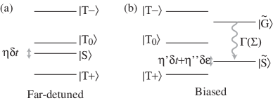
Figure 9: Level structures of the double dot system in the (a) far-detuned regime, with charge dephasing shown, and (b) near the charge transition with charge-based decay and dephasing.

As an example, a coherence between the $\left|S\right>$ and $\left|T_{m}\right>$ subspace in the far-detuned regime could be expected to decay due to the noise on $T_{c}$ according to

$$\langle e^{-\frac{i\eta}{\hbar}\int_{0}^{\tau}du^{\prime}\delta T_{c}(u^{\prime})}\rangle=\exp(-\eta^{2}\int d\omega\ S_{T_{c}}(\omega)\frac{\sin^{2}(\tau\omega/2)}{(\omega/2)^{2}})$$ (41)

While we consider a variety of noise sources in Appendix B, it is instructive here to take the case of white noise spectrum with $S_{T_{c}}=\gamma_{0}/2\pi$. It leads to exponential decay of coherences between $\left|S\right>$ and states of the $\left|T_{m}\right>$ subspace with a constant $\gamma_{T_{c}}=\eta^{2}\gamma_{0}$. In general, as $\eta\ll 1$, this decay will be negligible.

The charge transition will have stronger dephasing when compared with the far-detuned regime. In addition to inelastic decay of the excited adiabatic state to the ground adiabatic state, the system is susceptible to fluctuations in both $\epsilon$ and $T_{c}$, as $J$ is potentially large and strongly dependent on gate parameters. In so far as the power spectra associated with $T_{c}$ and $\epsilon$ have no appreciable spectral components at frequencies of order $\epsilon$, the excitation/relaxation terms between $\left|\tilde{G}\right>$ and $\left|\tilde{S}\right>$ may be neglected. Then we may restrict considerations to dephasing of coherence between the subspace of $\left|T_{m}\right>$ and the state $\left|\tilde{S}\right>$, and write the effective Hamiltonian as

$$V_{11-02}=[\eta^{\prime}\delta T_{c}(\tau)+\eta^{\prime\prime}\delta\epsilon(\tau)][\sum_{m}|T_{m}\rangle\!\langle T_{m}|-|\tilde{S}\rangle\!\langle\tilde{S}|]/2$$ (42)

with $\eta^{\prime}=\frac{2T_{c}}{\epsilon/2+\epsilon}$ and $\eta^{\prime\prime}=\frac{1}{2}(1+\frac{\epsilon}{\epsilon/2+\epsilon})$. The accompanying noise is given again by Eqn. 41, but with $\eta=\sqrt{(\eta^{\prime})^{2}+(\eta^{\prime\prime})^{2}}$ and the power spectrum replaced with

$$S_{11-02}(\omega)=\left(\frac{\eta^{\prime}}{\eta}\right)^{2}S_{T_{c}}(\omega)+\left(\frac{\eta^{\prime\prime}}{\eta}\right)^{2}S_{\epsilon}(\omega)$$ (43)

While $\eta^{\prime}$ may be small ($\eta\ll 1$), near the charge transition $\eta^{\prime\prime}$ is of order unity. This indicates that noise in the detuning parameter $\epsilon$ has significant repercussions for coherences between singlet and triplet states during exchange gate operation.

We consider charge-based dephasing for the exchange gate according to Eqn. 41. In all cases we assume the spectral function has a high-frequency cutoff $\gamma$ such that $\gamma\ll J$. This assumption prevents dephasing noise from producing population changes (relaxation) due to energy conservation. Additionally, we rewrite the expected probability of maintaining phase coherence (Eqn. 41) as

$$\exp(-\eta^{2}P)$$ (44)

where $P=\int d\omega\ S(\omega)\frac{\sin^{2}(\tau_{E}\omega/2)}{(\omega/2)^{2}}$ is set by the spectral function and the time of the exchange gate, $\tau_{E}$. This allows separation of the interaction strength ($\eta$) and the noise spectrum. Each spectrum considered has a normalization parameter $\nu$ such that $S(\omega)$ has units of inverse time.

We note that in general, the number of observable exchange oscillations will be limited by these dephasing processes. By finding $T_{2}=P^{-1}(\eta^{-2})$ the observable number of oscillations goes as $T_{2}J/\hbar$. When, for example, $S(\omega)=\Gamma/2\pi$, we may easily invert $P(t)$ and find $T_{2}=\eta^{-2}/\Gamma$.

Comparing the behavior of the ohmic and super-ohmic cases to the $1/f$ case (see Appendix B), the limiting value of $P$ for the super-ohmic case and the power law tail of the ohmic decay indicates that for small coupling parameter $\eta$, the super-exponential $1/f$ terms (going as a gaussian) will dominate at long times. For very short interaction times, all three will be less than the white noise contribution, which goes linearly in time. The different behaviors are shown in Fig. 10.

Figure 10: Decay of exchange oscillations for the four scenarios (clockwise from lower left): white noise, $1/f$, ohmic, and super-ohmic $(\omega^{2})$. White corresponds to probability 1 of ending in the initial state $\left|s,-s\right>$ after exchange interaction is on for a time $\tau_{E}$ (bottom axis), while black is probability 0 of ending in the initial state. Tunnel coupling is taken to be 10 $\mu$eV, and the spectral density ($\nu$) is chosen for similar behavior near $\epsilon=50\ \mu$eV. Note that $1/f$ terms increase decay in the slow oscillation limit, while increasing powers of $\omega$ (white noise=0, ohmic = 1, super-ohmic = 2) lead to more oscillations for smaller exchange energies.

This indicates that electrical control of exchange interactions in double dot systems may be relatively robust with respect to nuclear spin degrees of freedom. However, during the exchange gate, the system is susceptible to charge-related dephasing. The observed decay of oscillations of Ref. Petta et al., 2005a, in which the decay rate appears to match the exchange energy such that the number of exchange oscillations observed is independent of the detuning, is qualitatively similar to the behavior of oscillations in the presence of sub-ohmic noise. A more detailed experimental analysis of the noise will be required before a direct comparison between experiment and theory will be possible.

IV Exchange gates and echo techniques

The techniques of rapid adiabatic passage, slow adiabatic passage, and time-resolved control of the exchange interaction in the previous section have far reaching applications for quantum control of spins hanson07 . In this section, we consider how exchange gates can undo the effect of the quasi-static nuclear field, greatly reducing the deleterious effects of nuclear spins on electron spin coherences and allowing for electron spin measurements to determine nuclear spin correlation functions.

IV.1 Spin-echo in the singlet-triplet basis

Since the nuclear fields vary slowly on timescales compared to a typical pulse cycle time, a spin-echo pulse sequence can be used to refocus the spin singlet state. A spin-echo pulse sequence based on fast electrical control of the exchange interaction was demonstrated in Ref. Petta et al., 2005a. The experiment starts by using RAP to transfer $\left|(0,2)S\right>$ to $\left|S\right>$, preparing a separated singlet pair of electron spins. As demonstrated in the $T_{2}^{*}$ experiment, the hyperfine interaction mixes the singlet and triplet states on a 10 ns time scale. After a separation time $t_{S}$, a $\pi$ exchange pulse (SWAP) is performed by adjusting the detuning to a region with a finite exchange energy. The exchange energy is then set to zero by moving to the far-detuned regime for a time $t_{S^{\prime}}$, during which the singlet state refocuses.

The dephasing due to hyperfine interactions occurs by producing a relative, unknown phase between $\left|\uparrow\downarrow\right>$ and $\left|\downarrow\uparrow\right>$. Switching between these two states via exchange gates will produce an echo (recovery of the original state, $\left|S\right>$) if the waiting time before and after the $\rm SWAP$ operation is the same. In other words, the pseudo-spin of $\left|S\right>$ and $\left|T_{0}\right>$ (the $m_{s}=0$ subspace) is amenable to echo techniques using exchange interactions.

We will use the pulse sequence of Fig. 8c. In the far-detuned regime at finite field, $\left|S\right>$ and $\left|T_{0}\right>$ mix due to nuclei, as per the Hamiltonian of Eqn. 21. This mixing is driven by a relative constant, but unknown, energy, corresponding to the current value of

$$\hbar\hat{\omega}=\gamma_{e}(\hat{B}_{{\rm nuc},l,z}-\hat{B}_{{\rm nuc},r,z})~{}.$$ (45)

Within the corrections to the quasi-static approximation, $\hat{\omega}=\gamma_{e}(\delta\hat{B}_{l,z}(t)-\delta\hat{B}_{r,z}(t)$, where $\delta\hat{B}_{l(r),z}(t)$ are random, Gaussian variables described by Eqn. 12. For clarity, we rewrite it here:

$$\langle\hat{\omega}(t+\tau)\hat{\omega}(t)\rangle=\int d\omega\ S(\omega)e^{i\omega\tau}$$ (46)

For example, the singlet-singlet correlation function at finite field (Eqn. 37) is modified, noting that

$$\langle\cos^{2}(\int_{0}^{t}\hat{\omega}(t^{\prime})dt^{\prime})\rangle=\frac{1}{2}\left[1+\exp(-\int d\omega\ S(\omega)\frac{\sin^{2}(\tau\omega/2)}{(\omega/2)^{2}})\right]$$ (47)

For $S(\omega)$ with a high frequency cutoff below $1/\tau$, we can Taylor expand the $\sin$ term. Then, comparison with Eqn. 37 indicates:

$$T_{2}^{*}=\sqrt{\int d\omega\ S(\omega)}$$ (48)

Now, we consider how this result changes with the more complex sequence given by Fig. 8c, in particular its dependence on $\tau_{E}$ and $\tau_{S^{\prime}}$. If $\tau_{E}=0$, then nothing has changed from before, except now the system evolves according to $U_{\rm nuc}(\tau_{S^{\prime}})U_{\rm nuc}(\tau_{S})=U_{\rm nuc}(\tau_{S}+\tau_{S^{\prime}})$. However, what happens with finite $\tau_{E}$?

For our reduced two-level system, when $\tau_{E}\neq 0$ the effective Hamiltonian during this stage is given by

$$H_{eff,E}=\hbar\hat{\omega}\hat{\sigma}_{x}/2+J(\epsilon_{E})\hat{\sigma}_{z}/2\ .$$ (49)

where Pauli matrices with states $\left|S\right>,\left|T_{0}\right>$ as a psuedo- spin, in our logical basis defined above (i.e., $\sigma_{z}=|T_{0}\rangle\!\langle T_{0}|-|S\rangle\!\langle S|$). Taking the turn-on of finite $J$ to be instantaneous, the total evolution operator is

$$U(\tau_{S^{\prime}},\tau_{E},\tau_{S})=U_{\rm nuc}(\tau_{S^{\prime}})\exp(-iH_{eff,E}\tau_{E}/\hbar)U_{\rm nuc}(\tau_{S})\ .$$ (50)

When the exchange energy for the middle point satisfies $J(\epsilon_{E})\gg\gamma_{e}B_{\rm nuc}$, we approximate the middle term of the evolution operator by $U_{E}(\tau_{E})\approx\exp(-i\tau_{E}J(\epsilon_{E})\hat{\sigma}_{z}/2\hbar)$.

For now, taking $\hat{\omega}$ to be constant, at the end of the pulse sequence, the probability of returning to the state $\left|(0,2)S\right>$ ($C$) is given by

$$C={\rm Tr}_{{\rm nuc}}\left[\left|\left<0\right|e^{-i\tau_{S^{\prime}}\hat{\omega}\hat{\sigma}_{x}/2}e^{-i\tau_{E}J(\epsilon_{E})\hat{\sigma}_{z}/2\hbar}e^{-i\tau_{S}\hat{\omega}\hat{\sigma}_{x}/2}\left|0\right>\right|^{2}\right]~{}.$$ (51)

To see the analogy between this evolution and a spin echo experiment, we insert unity after the initial ket, i.e., $\left|0\right>=e^{iJ(\epsilon_{E})\hat{\sigma}_{z}/2\hbar}e^{-iJ(\epsilon_{E})(-1)/2\hbar}\left|0\right>$, as 0 is the -1 eigenstate of $\sigma_{z}$. The overall phase is irrelevant due to the absolute value terms, and so we rewrite the above as

$$C={\rm Tr}_{{\rm nuc}}\left[\left|\left<0\right|e^{-i\tau_{S^{\prime}}\hat{\omega}\hat{\sigma}_{x}/2}\left(e^{-i\tau_{E}J(\epsilon_{E})\hat{\sigma}_{z}/2\hbar}e^{-i\tau_{S}\hat{\omega}\hat{\sigma}_{x}/2}e^{i\tau_{E}J(\epsilon_{E})\hat{\sigma}_{z}/2\hbar}\right)\left|0\right>\right|^{2}\right]~{}.$$ (52)

The term in parenthesis, an exchange gate, is a rotation of angle $\theta_{E}=\tau_{E}J(\epsilon_{E})/\hbar$ about the $z$ axis of the psuedo-spin. It acts on the operator $U_{nuc}(\tau_{S})=e^{-i\tau_{S}\hat{\omega}\hat{\sigma}_{x}/2}$, flipping the sign of the $\sigma_{x}$ operator when $\theta_{E}=\pi$ (SWAP).

We can probe its effects by analogy with standard spin echo. For example, when $\theta_{E}=\pi$, we get $C=\frac{1}{2}[1+\exp(-\langle\omega^{2}\rangle(\tau_{S}-\tau_{S^{\prime}})^{2}/2)]$. This means the dephasing due to nuclei in the first half of the sequence is exactly undone when the rephasing time is equal ($\tau_{S}=\tau_{S^{\prime}}$). For fixed $\tau_{S}+\tau_{S^{\prime}}$, the probability of returning to the singlet state as a function of $\tau_{S}-\tau_{S^{\prime}}$ and $\tau_{E}$ should exhibit 50% mixing expected for dephasing when $|\tau_{S}-\tau_{S^{\prime}}|>T_{2}^{*}$, and when $\tau_{E}J/\hbar$ is not an odd integer multiple of $\pi$. For example, setting $\tau_{S}+\tau_{S^{\prime}}=100$ ns, and using $\epsilon_{E}$ such that $J(\epsilon_{E})=\hbar\gamma_{e}(20\ {\rm mT})$, the probability exhibits this behavior.

In practice, the instantaneous approximation breaks down in realistic situations, as does the $J\gg\gamma_{e}B_{\rm nuc}$ assumption. The former is easily fixed by noting that such a “Rabi” type pulse only has sensitivity to the integrated area, i.e., $\theta=\int J(\epsilon(t))dt$. The latter requires working with finite $\tau_{E}\Omega$. This effect has been considered in detail elsewhere Taylor and Lukin (2005).

IV.2 Probing nuclear spin dynamics through echo techniques

So far the analysis has worked entirely within the QSA. However, the echo sequence in principle reveals higher order dynamical information about the nuclear field and other noise sources. Effects of nuclear spin dynamics on electron spin decoherence has been considered by several authors de Sousa and Sarma (2003); Coish and Loss (2004); Yao et al. (2005); Witzel et al. (2005); Shenvi et al. (2005). We now consider the echo sequence with $\hat{\omega}(t)$ a Gaussian variable slowly varying in time. This allows a large range of possible noise sources and correlation functions to be considered.

Assuming (for the moment) that the exchange gate is of high fidelity and insensitive to the current value of $\hat{A}_{z}$, the measured result of the echo sequence is given by

$$C = |\left<0_{L}\right|\exp(i\int_{t_{S}}^{t_{S}+t_{S^{\prime}}}\hat{\omega}(t)dt\sigma_{x}/2$$ (53)

$$\ \ -i\int_{0}^{t_{S}}\hat{\omega}(t)dt\sigma_{x}/2)\left|0_{L}\right>|^{2}$$

$$= \cos^{2}[(\int_{t_{S}}^{t_{S}+t_{S^{\prime}}}\hat{\omega}(t)dt+\int_{0}^{t_{S}}\hat{\omega}(t)dt)/2]$$ (54)

$$= \frac{1}{4}[e^{-i\Xi}+e^{i\Xi}+2]$$ (55)

$$= \frac{1}{2}[e^{-\langle\Xi^{2}\rangle/2}+1]$$ (56)

where $\Xi=\int_{t_{S}}^{t_{S}+t_{S^{\prime}}}\hat{\omega}(t)dt+\int_{0}^{t_{S}}\hat{\omega}(t)dt$. The second moment of $\Xi$ is

$$\langle\Xi^{2}\rangle=\langle\Xi_{S^{\prime}}^{2}\rangle+\langle\Xi_{S}^{2}\rangle-2\langle\Xi_{S^{\prime}}\Xi_{S}\rangle$$ (57)

with $\langle\Xi_{S^{\prime}}^{2}\rangle=\int d\nu\ S(\nu)\frac{4}{\nu^{2}}\sin^{2}(t_{S^{\prime}}\nu/2)\simeq(t_{S^{\prime}}/T_{2}^{*})^{2}$ and similarly for $\Xi_{S}$. The cross term, corresponding to the correlations between the two frequencies, is

$$2\langle\Xi_{S^{\prime}}\Xi_{S}\rangle=\int d\nu\ S(\nu)\frac{\sin(t_{S}\nu/2)\sin(t_{S^{\prime}}\nu/2)}{(\nu/2)^{2}}e^{i(t_{S}+t_{S^{\prime}})\nu/2}~{}.$$ (58)

Finally, when $t_{S}=t_{S^{\prime}}$, the second moment is

$$\langle\Xi^{2}\rangle=2\int d\nu\ S(\nu)\frac{\sin^{2}(t_{S}\nu/2)}{(\nu/2)^{2}}[1-e^{it_{S}\nu}]~{}.$$ (59)

For low frequency noise, with cutoff $\gamma\simeq[\int d\nu\ \nu^{2}S(\nu)]^{1/2}\ll 1/t_{S}$, we obtain $\langle\Xi^{2}\rangle\simeq 2(t_{S})^{2}\times(t_{S}\gamma)^{2}$, or decay in the total wait time $2t_{S}$ with an effective time constant

$$T_{2,SE}=8^{1/4}(T_{2}^{*}/\gamma)^{1/2}\ .$$ (60)

Our evaluation has implicitly assumed that above the cutoff, $\gamma$, $S(\omega)$ dies off at least as $1/\omega^{3}$. We suggest that this is appropriate for interaction times on the order of microseconds—initial decay of the nuclear spin correlation function is quadratic. For longer interaction times, a different decay morphology (going as $\exp(-t^{3})$) could be observed.

Our predicted decay is consistent with the experiments of Ref. Petta et al., 2005a. In Refs. Witzel et al., 2005; Yao et al., 2005; Deng and Hu, 2005; Shenvi et al., 2005, $\gamma$ is of order 10 ms^-1, giving $T_{2,SE}=2\ \mu$s. However, addition exponential decay could be observed if the high frequency cut-off assumed above has a too-slow decay, going as $\omega^{-2-\epsilon}$ with $\epsilon<1$. Furthermore, higher order pulse sequences, such as Carr-Purcell, will likely allow for extensions of the echo signal to substantially longer timeswitzel07 ; zhang07 ; bhakta07 .

The experiments discussed in the previous sections demonstrate that the hyperfine interaction is efficient at dephasing an initially prepared spin singlet state on a 10 ns timescale. By using a simple spin-echo pulse sequence, this bare dephasing time was extended by over a factor of 100, to times $T_{2}$$>$1.2$\mu$s. Further experimental effort will be required to fully map out the nuclear correlation function and extend the lower bound on electron spin coherence times.

V Conclusions

We have shown how a model combining charge and spin interactions for two-electrons in a double quantum dot effectively describes the experimental results of Refs. Johnson et al., 2005; Petta et al., 2005a. By starting with the case of a single electron in a single dot, we employed the quasi-static approximation Burkard et al. (1999); Khaetskii et al. (2002); Coish and Loss (2004); Shenvi et al. (2005); Coish and Loss (2005); Witzel et al. (2005); Yao et al. (2005); Deng and Hu (2005), and considered its applicability to describing current experimental results.

The spin interactions with nuclear spins are extended to the double dot case, and two regimes emerge: the far-detuned regime, in which two electrons are in separate dots and interact with independent nuclear fields, and the charge transition, in which the two electrons may transition from a separated orbital state to a doubly-occupied, single-dot state.

This model was used to describe spin blockade, and we found spin blockade is broken by interactions with nuclei near zero magnetic field, explaining the experimental results of Johnson et al. (Ref. Johnson et al., 2005). A striking magnetic field dependance is derived, consistent with observed experimental behavior. This indicates that the dominant mechanism for spin blockade at finite magnetic field is trapping of the $m_{s}=\pm 1$ separated spin states, as their mixing with the charge-transition-allowed singlet $\left|G\right>$ is suppressed by finite Zeeman splitting. Observation of the breaking of spin blockade near zero field provides a sensitive measure of the magnitude of the random nuclear-spin-induced magnetic field.

Time-domain control of local potentials, achieved through manipulation of electrostatic depletion gates, provides powerful mechanisms for preparing and measuring spin singlets, as well as eigenstates of the nuclear field. These techniques have been exploited by Petta et al. to measure the effective dephasing of a two-spin entangled state, and to probe via coherent oscillations in the $m_{s}=0$ two-spin subspace the exchange interaction as controlled by gate voltages Petta et al. (2005a). Limiting mechanisms for such oscillations, due to charge fluctuations of indeterminate nature, are considered for a variety of environmental noise spectra.

Finally, we analyzed how controlled exchange interactions can protect the electron spin from the deleterious effect of nuclear spins by working within a two-spin subspace, putting in specific terms protocols previously conceived more generally. We expect the limiting mechanism for the rephasing of the two-spin states comes from corrections to the quasi-static approximation, and as such, spin-echo experiments provide a useful measure of the validity of this approximation.

Appendix A Adiabatic elimination for nuclear-spin-mediated inelastic decay

We will transform the superoperator (Eqn. 23) into the interaction picture, but first introduce matrix elements between the eigenstates of the quasi-static fields and the state $\left|S\right>$ occurring in the superoperator. For a single spin in a magnetic field $\vec{B}=B_{\rm nuc}(x,y,z)$ and $|B|=B_{\rm nuc}n$ (the roman variables $x,y,z,n$ are chosen such that the nuclear field contribution will be of order unity), the eigenstates may be written by rotation from spin states aligned with the $z$-axis ($\{\left|\uparrow\right>,\left|\downarrow\right>\}$):

$$\left(\begin{array}[]{c}\left|1/2\right>\\ \left|-1/2\right>\end{array}\right)=\lim_{x^{\prime}\rightarrow x^{+}}\frac{1}{\sqrt{2n(n+z)}}\left(\begin{array}[]{cc}n+z&x^{\prime}-iy\\ x^{\prime}+iy&-n-z\end{array}\right)\left(\begin{array}[]{c}\left|\uparrow\right>\\ \left|\downarrow\right>\end{array}\right)$$ (61)

The limit is taken only to remove the degenerate case of field anti-aligned with the $z$-axis, i.e., $\vec{B}=(0,0,-B)$, which would be degenerate for this matrix, and is implicit in what follows. The corresponding eigenvalues of the Hamiltonian are $\pm\hbar\Omega n/2$ in this notation.

Setting $\left|S\right>=(\left|\uparrow\downarrow\right>-\left|\downarrow\uparrow\right>)/\sqrt{2}$ and using the single spin transformations for $l$ and $r$ separately (with $\vec{B}^{l}=B_{\rm nuc}^{l}(x_{l},y_{l},z_{l}),|B^{l}|=n_{l}$ and similarly for $r$), we write

$$c_{1/2,1/2}=\left\langle\frac{1}{2},\frac{1}{2}\vphantom{S}\right.\left|\vphantom{\frac{1}{2},\frac{1}{2}}S\right\rangle = \frac{1}{\mathcal{N}}\left[(x_{l}+iy_{l})(n_{r}+z_{r})-(n_{l}+z_{l})(x_{l}+iy_{l})\right]$$ (62)

$$c_{1/2,-1/2}=\left\langle\frac{1}{2},-\frac{1}{2}\vphantom{S}\right.\left|\vphantom{\frac{1}{2},-\frac{1}{2}}S\right\rangle = \frac{1}{\mathcal{N}}\left[-(n_{l}+z_{l})(n_{r}+z_{r})-(x_{l}+iy_{l})(x_{r}-iy_{r})\right]$$ (63)

$$c_{-1/2,1/2}=\left\langle-\frac{1}{2},\frac{1}{2}\vphantom{S}\right.\left|\vphantom{-\frac{1}{2},\frac{1}{2}}S\right\rangle = -c_{1/2,-1/2}^{*}$$ (64)

$$c_{-1/2,-1/2}=\left\langle-\frac{1}{2},-\frac{1}{2}\vphantom{S}\right.\left|\vphantom{-\frac{1}{2},-\frac{1}{2}}S\right\rangle = c_{1/2,1/2}^{*}$$ (65)

$${\rm and}\ {\mathcal{N}} = \sqrt{8n_{l}n_{r}(n_{l}+z_{l})(n_{r}+z_{r})}$$ (66)

It is convenient to define $c_{++}=c_{1/2,1/2}$ and $c_{+-}=c_{1/2,-1/2}$ as the spin-aligned and spin-anti-aligned coefficients, respectively. This allows us to express $\left|S\right>$ occurring in Eqn. 23 in terms of the eigenstates of the Hamiltonian as

$$\left|S\right>=\sum_{s,s^{\prime}}c_{s,s^{\prime}}\left|s,s^{\prime}\right>=c_{++}\left|\frac{1}{2},\frac{1}{2}\right>+c_{+-}\left|\frac{1}{2},-\frac{1}{2}\right>-c_{+-}^{*}\left|-\frac{1}{2},\frac{1}{2}\right>+c_{++}^{*}\left|-\frac{1}{2},-\frac{1}{2}\right>$$ (67)

In the interaction picture, each eigenstate $\left|s,s^{\prime}\right>$ evolves according to

$$\left|s,s^{\prime}(t)\right>=e^{-iE_{s,s^{\prime}}t/\hbar}\left|s,s^{\prime}\right>=e^{-i(sn_{l}\gamma_{e}B_{{\rm nuc},l}+s^{\prime}n_{r}\gamma_{e}B_{{\rm nuc},r})t}\ ,$$ (68)

and $\left|S(t)\right>=\sum_{s,s^{\prime}}c_{s,s^{\prime}}\left|s,s^{\prime}(t)\right>$.

With these results, the louivillian may be put into the interaction picture:

$$\dot{\tilde{\rho}} = \Gamma(\epsilon)/2\sum_{s,s^{\prime},r,r^{\prime}}c_{s,s^{\prime}}c_{r,r^{\prime}}^{*}e^{i[(r-s)n_{l}\gamma_{e}B_{{\rm nuc},l}+(r^{\prime}-s^{\prime})n_{r}\gamma_{e}B_{{\rm nuc},r}]t}L_{s,s^{\prime},r,r^{\prime}}[\tilde{\rho}]$$ (69)

$${\rm where}\ L_{s,s^{\prime},r,r^{\prime}}[\tilde{\rho}] = \left[|s,s^{\prime}\rangle\!\langle r,r^{\prime}|\tilde{\rho}+\tilde{\rho}|s,s^{\prime}\rangle\!\langle r,r^{\prime}|-2|G\rangle\!\langle r,r^{\prime}|\tilde{\rho}|s,s^{\prime}\rangle\!\langle G|\right]$$ (70)

So far, this result is exact within the QSA.

When $\Gamma(\epsilon)\ll\gamma_{e}B_{{\rm nuc},l},\gamma_{e}B_{{\rm nuc},r}$, the exponential phase terms of Eqn. 69 oscillate substantially faster than $\tilde{\rho}$ evolves. Adiabatic elimination becomes an appropriate approximation when we may neglect quickly rotating terms, i.e., if we may neglect certain degenerate cases, such as situations with $|n_{l}\gamma_{e}B_{{\rm nuc},l}-n_{r}\gamma_{e}B_{{\rm nuc},r}|\lesssim\Gamma(\epsilon)$. In addition, we are implicitly assuming that $\Gamma(\epsilon)\simeq\Gamma(\epsilon+E_{s,s^{\prime}}-E_{r,r^{\prime}})$, which is appropriate for large $\epsilon$ and smooth phonon density of states.

More explicitly, we can average each term of over several spin rotations and make a Born approximation:

$$e^{i[(r-s)n_{l}\gamma_{e}B_{{\rm nuc},l}+(r^{\prime}-s^{\prime})n_{r}\gamma_{e}B_{{\rm nuc},r}]t}L_{s,s^{\prime},r,r^{\prime}}[\tilde{\rho}(t)]\rightarrow\left[\frac{1}{\tau}\int_{t-\tau}^{t}e^{i[(r-s)n_{l}\gamma_{e}B_{{\rm nuc},l}+(r^{\prime}-s^{\prime})n_{r}\gamma_{e}B_{{\rm nuc},r}]t^{\prime}}dt^{\prime}\right]L_{s,s^{\prime},r,r^{\prime}}[\tilde{\rho}(t)]$$ (71)

The time averaging for a given $s,s^{\prime},r,r^{\prime}$ is straightforward so long as $n_{l}B_{{\rm nuc},l}\neq n_{r}B_{{\rm nuc},r}$, giving

$$\lim_{\tau\rightarrow\infty}\frac{1}{\tau}\int_{t-\tau}^{t}e^{i[(r-s)n_{l}\gamma_{e}B_{{\rm nuc},l}+(r^{\prime}-s^{\prime})n_{r}\gamma_{e}B_{{\rm nuc},r}]t^{\prime}}dt^{\prime}=\delta_{s,r}\delta_{s^{\prime},r^{\prime}}$$ (72)

Thus terms with quickly varying phase go to zero.

Appendix B Dephasing power spectra

We now evaluate dephasing in exchange gates due to charge fluctuations for a variety of spectral functions. The error should go as $[1-\exp(-\eta^{2}P)]/2$, where the value $\eta$ depends only on the detuning parameter. The impact of the particular spectral function is encompassed in $P=\int d\omega\ S(\omega)\frac{\sin^{2}(t\omega/2)}{(\omega/2)^{2}}$. We have assumed that $S(\omega)$ has a high frequency cutoff $\gamma\ll 1/t$.

B.1 White noise

We set $S(\omega)=\frac{\nu}{2\pi}e^{-\omega/\gamma}$. Then we can evaluate

$$P=\frac{\nu}{2\pi}\int d\omega\ \frac{\sin^{2}(\omega t/2)}{(\omega/2)^{2}}e^{-\omega/\gamma}\approx\nu t\ .$$ (73)

This indicates the expected exponential decay of coherence due to white noise dephasing.

B.2 $1/f$ noise

With $S(\omega)=\nu^{2}/\omega$ and frequency cutoffs $B<\omega<\gamma\ll 1/t$,

$$P=2\log[\gamma/B](\nu t)^{2}\ .$$ (74)

For a bath of $1/f$ distributed fluctuators, the initial dephasing is quadratic in the time of interaction, and increases as the measurement timescale ($1/B$) increases. At long times, the decay is gaussian, with super-exponential suppression of coherence.

B.3 Ohmic noise

Taking $S(\omega)=g\omega e^{-\omega/\gamma}$, evaluation of $P$ is possible, giving

$$P=2g\log[1+(\gamma t)^{2}]\ .$$ (75)

When considered in the decay function $\exp(-\eta^{2}P)$, this gives a non-exponential decay law, $\exp(-\eta^{2}P)=[1+(\gamma t)^{2}]^{-2g\eta^{2}}$. In the short time limit, this is quadratic decay, going as $1-2(g\eta^{2})(\gamma t)^{2}+O((\gamma t)^{4})$, while the long time behavior is a power law with power $-4g\eta^{2}$.

B.4 Super-ohmic noise

For the final spectral function considered here, we set $S(\omega)=\nu^{1-\zeta}\omega^{\zeta}e^{-\omega/\gamma}$ where $\zeta>1$ indicates super-ohmic noise. Evaluation of $P$ proceeds in a straightforward manner, giving

$$P = \frac{1}{4}\Gamma(\zeta-1)\left(\frac{\nu}{\gamma}\right)^{1-\zeta}\Big{\{}1-$$ (76)

$$\ \ \left[1+(\gamma t)^{\frac{1}{2}-\frac{\zeta}{2}}\right]\cos[(\zeta-1)\tan^{-1}(\gamma t)]\Big{\}}\ .$$

where $\Gamma(x)$ is the gamma function. This type of decay has a limiting value of

$$\lim_{t\rightarrow\infty}P=4\Gamma(\zeta-1)\left(\frac{\nu}{\gamma}\right)^{1-\zeta}$$ (77)

and short time behavior according to

$$P(t)=2\zeta(\zeta-1)\Gamma(\zeta-1)\left(\frac{\nu}{\gamma}\right)^{1-\zeta}(\gamma t)^{2}+O((\gamma t)^{4})\ .$$ (78)

For visual comparison, we calculate the expected, observable Rabi oscillations using SAP as a function of time at finite exchange ($t_{E}$) and at detuning $\epsilon$ in Fig. 10. In essence, increasing the exponent of the noise spectra (from $1/\omega$ to constant to $\omega^{\zeta}$) leads to more oscillations as detuning is made more negative, i.e., as the admixture of charge decreases.

References

- Awschalom et al. (2002) D. D. Awschalom, N. Samarth, and D. Loss, eds., Semiconductor Spintronics and Quantum Computation (Springer-Verlag, Berlin, 2002).
- (2) D. D. Awschalom and M. E. Flatté, Nat. Phys. 3, 153 (2007).
- Loss and DiVincenzo (1998) D. Loss and D. P. DiVincenzo, Phys. Rev. A 57, 120 (1998).
- Imamoglu et al. (1999) A. Imamoglu, D. D. Awschalom, G. Burkard, D. P. DiVincenzo, D. Loss, M. Sherwin, and A. Small, Phys. Rev. Lett. 83, 4204 (1999).
- Taylor et al. (2005a) J. M. Taylor, H.-A. Engel, W. Dür, A. Yacoby, C. M. Marcus, P. Zoller, and M. D. Lukin, Nature Physics 1, 177 (2005a).
- (6) R. Hanson, L. P. Kouwenhoven, J. P. Petta, S. Tarucha, L. M. K. Vandersypen, cond-mat/0610433.
- Golovach et al. (2004) V. N. Golovach, A. Khaetskii, and D. Loss, Phys. Rev. Lett. 93, 016601 (2004).
- Khaetskii and Nazarov (2000) A. V. Khaetskii and Y. V. Nazarov, Phys. Rev. B 61, 12639 (2000).
- Khaetskii and Nazarov (2001) A. V. Khaetskii and Y. V. Nazarov, Phys. Rev. B 64, 125316R (2001).
- Burkard et al. (1999) G. Burkard, D. Loss, and D. P. DiVincenzo, Phys. Rev. B 59, 2070 (1999).
- Merkulov et al. (2002) I. A. Merkulov, A. L. Efros, and M. Rosen, Phys. Rev. B 65, 205309 (2002).
- Khaetskii et al. (2002) A. V. Khaetskii, D. Loss, and L. Glazman, Phys. Rev. Lett. 88, 186802 (2002).
- Erlingsson and Nazarov (2002) S. I. Erlingsson and Y. V. Nazarov, Phys. Rev. B 66, 155327 (2002).
- de Sousa and Sarma (2003) R. de Sousa and S. Das Sarma, Phys. Rev. B 68, 115322 (2003).
- Coish and Loss (2004) W. A. Coish and D. Loss, Phys. Rev. B 70, 195340 (2004).
- Schulten and Wolynes (1978) K. Schulten and P. G. Wolynes, J. Chem. Phys. 68, 3292 (1978).
- Yao et al. (2005) W. Yao, R.-B. Liu, and L. J. Sham, Phys. Rev. B 74, 195301 (2006).
- Deng and Hu (2005) C. Deng and X. Hu, Phys. Rev. B 73, 241303 (2006).
- Bracker et al. (2005) A. S. Bracker, E. A. Stinaff, D. Gammon, M. E. Ware, J. G. Tischler, A. Shabaev, A. L. Efros, D. Park, D. Gershoni, V. L. Korenev, I. A. Merkulov,, Phys. Rev. Lett. 94, 047402 (2005).
- Johnson et al. (2005) A. C. Johnson, J. Petta, J. M. Taylor, M. D. Lukin, C. M. Marcus, M. P. Hanson, and A. C. Gossard, Nature 435, 925 (2005).
- Petta et al. (2005a) J. R. Petta, A. C. Johnson, J. M. Taylor, E. Laird, A. Yacoby, M. D. Lukin, and C. M. Marcus, Science 309, 2180 (2005a).
- Koppens et al. (2005) F. H. L. Koppens, J. A. Folk, J. M. Elzerman, R. Hanson, L. H. Willems van Beveren, I. T. Vink, H.-P. Tranitz, W. Wegscheider, L. P. Kouwenhoven, and L. M. K. Vandersypen, Science 309, 1346 (2005).
- (23) F. H. L. Koppens, C. Buizert, K. J. Tielrooij, I. T. Vink, K. C. Nowack, T. Meunier, L. P. Kouwenhoven, and L. M. K. Vandersypen, Nature 442, 766 (2006).
- (24) E. A. Laird, J. R. Petta, A. C. Johnson, C. M. Marcus, A. Yacoby, M. P. Hanson, A. C. Gossard, Phys. Rev. Lett. 97, 056801 (2006).
- Schliemann et al. (2001) J. Schliemann, D. Loss, and A. H. MacDonald, Phys. Rev. B 63, 085311 (2001).
- Taylor et al. (2005b) J. M. Taylor, W. Dür, P. Zoller, A. Yacoby, C. M. Marcus, and M. D. Lukin, Phys. Rev. Lett. 94, 236803 (2005b).
- Coish and Loss (2005) W. A. Coish and D. Loss, Phys. Rev. B 72, 125337 (2005).
- Witzel et al. (2005) W. M. Witzel, R. de Sousa, and S. Das Sarma, Phys. Rev. B 72, 161306 (2005).
- Shenvi et al. (2005) N. Shenvi, R. de Sousa, and K. B. Whaley, Phys. Rev. B 71, 224411 (2005).
- Hu and Sarma (2005) X. Hu and S. Das Sarma, Phys. Rev. Lett. 96, 100501 (2006).
- Klauser et al. (2005) D. Klauser, W. A. Coish, and D. Loss, Phys. Rev. B 73, 205302 (2006).
- Brandes and Kramer (1999) T. Brandes and B. Kramer, Phys. Rev. Lett. 83, 3021 (1999).
- Fujisawa et al. (2001) T. Fujisawa, Y. Tokura, and Y. Hirayama, Phys. Rev. B. (Rapid Comm.) 63, 081304 (2001).
- Brandes and Vorrath (2002) T. Brandes and T. Vorrath, Phys. Rev. B 66, 075341 (2002).
- de Sousa and Das Sarma (2003) R. de Sousa and S. Das Sarma, Phys. Rev. B 67, 033301 (2003).
- Hanson et al. (2003) R. Hanson, B. Witkamp, L. M. K. Vandersypen, L. H. W. van Beveren, J. M. Elzerman, and L. P. Kouwenhoven, Phys. Rev. Lett. 91, 196802 (2003).
- Kroutvar et al. (2004) M. Kroutvar, Y. Ducommun, D. Heiss, M. Bichler, D. Schuh, G. Abstreiter, and J. J. Finley, Nature 432, 81 (2004).
- Paget et al. (1977) D. Paget, G. Lampel, B. Sapoval, and V. Safarov, Phys. Rev. B 15, 5780 (1977).
- (39) W. Witzel and S. Das Sarma, Phys. Rev. B 74, 035322 (2006).
- Al-Hassanieh et al. (2006) K. A. Al-Hassanieh, V. V. Dobrovitski, E. Dagotto, and B. N. Harmon, Phys. Rev. Lett. 97, 037204 (2006).
- (41) W. G. van der Wiel, S. De Franceschi, J. M. Elzerman, T. Fujisawa, S. Tarucha and L. P. Kouwenhoven, Rev. Mod. Phys. 75, 1 (2003).
- Ono and Tarucha (2004) K. Ono and S. Tarucha, Phys. Rev. Lett. 92, 256803 (2004).
- Taylor et al. (2003) J. M. Taylor, A. Imamoglu, and M. D. Lukin, Phys. Rev. Lett. 91, 246802 (2003).
- Erlingsson et al. (2003) S. I. Erlingsson, O. N. Jouravlev, and Y. V. Nazarov, Phys. Rev. B72, 033301 (2005).
- (45) M. S. Rudner, L. S. Levitov, cond-mat/0609409.
- (46) G. Ramon, X. Hu, cond-mat/0610585.
- (47) Erlingsson, S. I., Nazarov, Y. V. and Fal’ko, V. I., Phys. Rev. B 64, 195306 (2001).
- (48) O. N. Jouravlev and Yu. V. Nazarov, Phys. Rev. Lett. 96, 176804 (2006)
- Elzerman et al. (2004) J. M. Elzerman, R. Hanson, L. H. W. van Beveren, B. Witkamp, L. M. K. Vandersypen, and L. P. Kouwenhoven, Nature 430, 431 (2004).
- (50) T. Meunier, I. T. Vink, L. H. Willems van Beveren, K-J. Tielrooij, R. Hanson, F. H. L. Koppens, H. P. Tranitz, W. Wegscheider, L. P. Kouwenhoven, and L. M. K. Vandersypen, cond-mat/0609726.
- (51) R. Hanson, L. H. Willems van Beveren, I. T. Vink, J. M. Elzerman, W. J. M. Naber, F. H. L. Koppens, L. P. Kouwenhoven, L. M. K. Vandersypen, Phys. Rev. Lett. 94, 196802 (2005).
- Petta et al. (2005b) J. R. Petta, A. C. Johnson, A. Yacoby, C. M. Marcus, M. P. Hanson, and A. C. Gossard, Phys. Rev. B. 72, 161301 (2005b).
- Fujisawa et al. (1998) T. Fujisawa, T. H. Oosterkamp, W. G. van der Wiel, B. W. Broer, R. Aguado, S. Tarucha, and L. P. Kouwenhoven, Science 282, 932 (1998).
- Taylor and Lukin (2005) J. M. Taylor and M. D. Lukin, Quant. Inf. Proc. 5, 503 (2006).
- (55) M. Stopa and C. M. Marcus, cond-mat/0604008.
- (56) R. Hanson and G. Burkard, Phys. Rev. Lett. 98, 050502 (2007).
- (57) W. M. Witzel and S. Das Sarma, Phys. Rev. Lett. 98, 077601 (2007).
- (58) W. Zhang, V. Dobrovitski, L. F. Santos, L. Viola, B. N. Harmon, cond-mat/0701507.
- (59) D. D. Bhaktavatsala, V. Ravishankar, V. Subrahmanyan, quant-ph/0702035.