Deconfined criticality, runaway flow in the two-component scalar electrodynamics and weak first-order superfluid-solid transitions

Abstract

We perform a comparative Monte Carlo study of the easy-plane deconfined critical point (DCP) action and its short-range counterpart to reveal close similarities between the two models for intermediate and strong coupling regimes. For weak coupling, the structure of the phase diagram depends on the interaction range: while the short-range model features a tricritical point and a continuous U(1)$\times$U(1) transition, the long-range DCP action is characterized by the runaway renormalization flow of coupling into a first (I) order phase transition. We develop a “numerical flowgram” method for high precision studies of the runaway effect, weakly I-order transitions, and polycritical points. We prove that the easy-plane DCP action is the field theory of a weakly I-order phase transition between the valence bond solid and the easy-plane antiferromagnet (or superfluid, in particle language) for any value of the weak coupling strength. Our analysis also solves the long standing problem of what is the ultimate fate of the runaway flow to strong coupling in the theory of scalar electrodynamics in three dimensions with U(1)$\times$U(1) symmetry of quartic interactions.

I Introduction

Critical properties of systems described by several complex fields coupled to the gauge field have a long history of studies and are relevant for numerous problems in physics which include normal-superfluid transitions in multi-component neutral or charged liquids (see, e.g. Halperin2 ; Brezin ; Chen ; Babaev ), superfluid–valence-bond solid (SF-VBS) transitions in lattice models dcp1 ; dcp2 ; dcp3 , the Higgs mechanism in particle physics Higgs , etc. Recently, the authors of Refs. dcp1 ; dcp2 ; Motrunich argued that the SF–VBS transition in a $(2+1)$-dimensional system is an example of a qualitatively new type of quantum criticality (“decondined criticality”) that does not fit the Ginzburg-Landau-Wilson (GLW) paradigm. As suggested in reference Zoller_Fisher , an experimental realization of the SF-VBS transition is possible in the system of ultracold atoms trapped in optical lattice. If true, the significance of the claim that DCP opens a new era in the theory of phase transitions is hard to overestimate. The study of the SF-VBS transition within the DCP theory framework, and the closely related problem of the runaway flow to strong coupling in the theory of scalar quantum electrodynamics in three dimensions (3D) Halperin2 ; Brezin ; Chen is the main focus of this work.

We also discuss a short-range analog of the DCP action, namely, the model describing lattice phases of the two-component Bose-Hubbard (BH2) system with large integer filling factors twocolor . The only difference between the DCP and BH2 models lies in the interaction range. The DCP action is characterized by a long-range Coulomb type interaction, which is replaced with the contact $\delta$-functional form in the BH2 analog. Despite this difference, the gross features of the phase diagram are surprisingly similar in both models, especially in the regimes of intermediate and strong coupling between the two field components. Even quantitatively, the phase diagrams are nearly indistinguishable, see Fig. 2. Both feature a bicritical point (BP) above which there are three phases: a superfluid (SF), a paired phase and an insulator. The superfluid is characterized by the order parameters for two complex scalar fields, $\langle\psi_{1}\rangle\neq 0,\,\langle\psi_{2}\rangle\neq 0$. In the paired phase the order parameter is $\langle\psi^{*}_{1}\psi_{2}\rangle\neq 0$ while $\langle\psi_{1}\rangle=\langle\psi_{2}\rangle=0$. In the context of the DCP theory, the paired phase is associated with the valence-bond supersolid (SFS); within the BH2 model twocolor it corresponds to the super-counter-fluid (SCF) phase describing pairing between particles of one component and holes of another SCF . Finally, the insulating phase represents the VBS state in the DCP theory and the Mott insulator (MI) state in the BH2 model. In this phase all off-diagonal order parameters are zero.

The crucial difference between the two models is seen below the bicritical point BP, where direct transitions from insulator to SF take place. In the DCP action this line describes the SF-VBS transformation. An implicit assumption made in Refs. dcp1 ; dcp2 ; Motrunich was that as the interaction constant between the field components, $g$, weakens down to $g=0$ (where DCP and BH2 actions become identical and describe two decoupled XY-models), there exists a lower tricritical point (TP) $g_{LTP}>0$ below which the VBS-SF transition becomes continuous. Since lower TP does exist in the short-range BH2 model twocolor , the expectation was that both models have essentially identical phase diagrams, with only one important difference— in the short-range case the continuous transition below lower TP accounts for the U(1)$\times$U(1) universality, while the continuous transition in the DCP action for $0<g<g_{LTP}$ would be in the new “deconfined” universality class. However, as we suggested earlier YKIS and now clearly demonstrate below, no such lower TP exists in the DCP action and the line of I-order SF-VBS transitions extends all the way to $g\to 0$.

The tool we introduce for studying subtle features of the phase diagram is the numerical flowgram method. It is based on scaling properties of quantities similar to Binder cummulants Binder and turns out to be much more adequate for analyzing weakly I-order transitions than the conventional method based on the bimodal shape of the energy/action distribution and hysteresis loops. The flowgram technique can also be used for systematic identification of polycritical points. To the best of our knowledge no other method can achieve this goal with comparable accuracy. First, we construct the flowgram for the BH2 model and demonstrate its efficiency for those parts of the phase diagram which can be reliably identified by more conventional methods. Next, we apply the new method to the most controversial region of the BH2 phase diagram between BP and upper TP, which we failed to resolve in the previous study twocolor . The existence of upper TP proves that the mean field does reproduce the topology of the phase diagram for the short-range model correctly, with the reservation that fluctuation-induced effects significantly shorten the interval between the bicritical and the upper tricritical points.

Finally, we apply the flowgram method to the self-dual version of the DCP action Motrunich . We have identified the bicritical and the upper tricritical points, but no lower TP has been found. We directly observe the runaway flow to strong coupling and prove that its ultimate fate is a I-order transition. More specifically, for small $g$, we observe data collapse with respect to the coupling strength rescaled by the system size $L$. This collapse indicates the existence of an effective long-range coupling $g_{\rm eff}(L)$ and proves that it is never weak in the $L\to\infty$ limit: no matter how small is $g$ at short scales it always gets renormalized to $g_{\rm eff}\sim 1$ where the I-order transition takes place. Perfect data collapse continuously relating small $g$ to one for which I-order transition is observed at accessible sizes provides crucial evidence against lower TP and in support of the claim that the direct VBS-SF transition is always weakly I-order in accordance with the Ginzburg-Landau-Wilson paradigm YKIS .

On one hand, our results represent the first solution of the long-standing runaway problem for the two-component field-theory in question. On the other hand, they explain the outcome of recent numerical simulations which report either difficulties with finite-size scaling of the data Sandvik or weakly I-order transitions weak1 in microscopic models of the SF-VBS transition.

II DCP action and its short-range counterpart

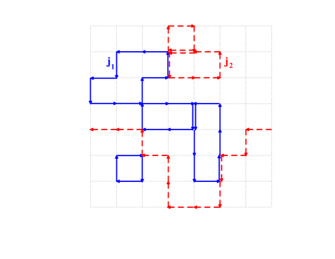
Figure 1: (Color online). A typical configuration of currents for the two-component $j$-current model. The configuration space consists of arbitrary number of closed oriented loops which are allowed to overlap and intersect. The current ${\bf j}_{a=1,2}$ is defined as an algebraic sum of all same-type arrows on the corresponding bond.

There are many equivalent formulations of the action describing multi-component scalar fields coupled by the Abelian gauge field dcp1 ; Babaev ; Motrunich . In what follows we will concentrate on the case of two identical non-convertible components and will employ the integer-current lattice representation which can be viewed as either a high-temperature expansion for XY models in three dimensions, or as a path-integral (world-line) representation of the interacting quantum system in discrete imaginary time in $(d+1)=3$ dimensions. The DCP action is explicitly symmetric with respect to exchanging the components. After the gauge field is integrated out, it reads

$$S_{2}^{(l)}=U{\bf j}_{1{\bf r}}^{2}+U{\bf j}_{2{\bf r}}^{2}+gQ_{{\bf r}-{\bf r}^{\prime}}\left({\bf j}_{1{\bf r}}+{\bf j}_{2{\bf r}}\right)\cdot\left({\bf j}_{1{\bf r}^{\prime}}+{\bf j}_{2{\bf r}^{\prime}}\right)\;,$$ (1)

with $U>0,\,g>0$. The lattice Fourier transform of the long-range interaction potential $Q_{{\bf r}-{\bf r}^{\prime}}$ is given by $Q_{\bf q}=1/\sum_{\mu}\sin^{2}(q_{\mu}/2)$, which implies the asymptotic form $Q(r\to\infty)\sim 1/r$. The summation over sites of the simple cubic space-time lattice with periodic boundary conditions, ${\bf r}$, is assumed. Integer currents ${\bf j}_{a{\bf r}}=(j_{a{\bf r}})_{\mu}$ with $a=1,2$ and $\mu=x,y,\tau$ are defined on the lattice bonds and are subject to the zero-divergence, $\nabla{\bf j}=0$, constraint, i.e. the configuration space of $j$-currents is that of closed oriented loops, see Fig. 1. In terms of particle world lines, currents in the time direction represent occupation number fluctuations away from the commensurate filling, and currents in the spatial directions represent hopping events. In the discussion of the SF–VBS transition, $j_{1}$ and $j_{2}$ currents in the DCP action represent world lines of spinons which are VBS vortices carrying fractional particle charge $\pm 1/2$ dcp1 ; dcp2 . The insulating VBS state is characterized by small current loops; the corresponding spinon order parameter, $\psi_{a},\,a=1,2$, is zero in this phase. When spinon world lines proliferate and grow macroscopically large, the system enters the superfluid state. The paired phase (SFS) occurs at large $g$, when only loops in the ${\bf j}_{1}-{\bf j}_{2}$ channel grow macroscopically large. Since bound pairs of spinons with opposite vorticity make particle and hole excitations, the SFS state is a superfluid with the solid VBS order, i.e. a supersolid.

As discussed above, many features of the DCP action are remarkably similar to those of a more conventional two-component Bose-Hubbard model twocolor with the short-range interaction potential

$$S_{2}^{(s)}=U\>{\bf j}_{1{\bf r}}^{2}+U\>{\bf j}_{2{\bf r}}^{2}+V\>\left({\bf j}_{1{\bf r}}+{\bf j}_{2{\bf r}}\right)^{2}\;,$$ (2)

with $U>0,\,V>0$. Phase diagrams for the long- and short-range actions are shown in Fig. 2. Different phases are identified in terms of loop sizes for ${\bf j}_{1}$ and ${\bf j}_{2}$ currents similar to the discussion given above: the Mott insulator (MI) is characterized by small ${\bf j}_{1}$- and ${\bf j}_{2}$-loops, in the two-component SF there are macroscopically large ${\bf j}_{1}$- and ${\bf j}_{2}$-loops, and in the SCF state only ${\bf j}_{1}-{\bf j}_{2}$ loops are macroscopically large.

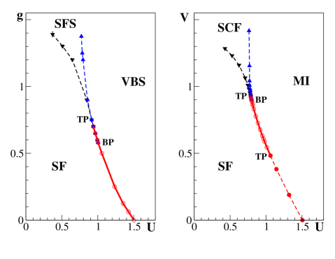
Figure 2: (Color online). Phase diagrams of the long-range (left panel), Eq. (1), and short-range (right panel), Eq. (2), actions. Bold solid lines indicate the I-order phase transition. Error bars are shown but are typically much smaller than symbol sizes.

Previous Monte Carlo data for the BH2 model (2) did not agree with the mean field theory which describes the system in terms of three fields — $\psi_{1,2}$ for each component and $\Phi$ for the paired field twocolor . Omitting gradient terms the mean-field action is given by:

$$S_{MF}={1\over 2}\big{[}r(|\psi_{1}|^{2}+|\psi_{2}|^{2}) + r_{m}|\Phi|^{2}\big{]}+{1\over 4}\big{[}U_{\psi}(|\psi_{1}|^{4}+|\psi_{2}|^{4})+U_{\phi}|\Phi|^{4}\big{]}$$ (3)

$$- \gamma(\Phi\psi^{*}_{1}\psi_{2}+\rm{c.c.})\;,$$

where $r,\,r_{m},\,U_{\psi}>0,\,U_{\phi}>0,\,\gamma$ are some effective coefficients which depend on the bare coupling parameters $U,\,V$ in the action (2). Trivial minimization of (3) with respect to the order parameter fields results in the phase diagram which can be formulated in terms of two dimensionless variables $\sim r$ and $\sim r_{m}$, with all other coefficients rescaled to become unity twocolor . A sketch of the diagram is presented in Fig. 3. It features a continuous SCF-MI transition, which terminates at BP point, as well as I-order MI-SF and SCF-SF transitions. The SCF-SF transition starts as a first-order line at BP and goes up to upper TP. Then, it continues as a second (II) order line for larger values of $V$. Similarly, the MI-SF transition is of I-order type between BP and lower TP. Then, it continues as a II-order $U(1)\times U(1)$ transition line towards the $V=0$ point where the components become decoupled. The length of the I-order line along the SCF-SF boundary is predicted to be about two times shorter than that along the MI-SF line, see Fig. 3.

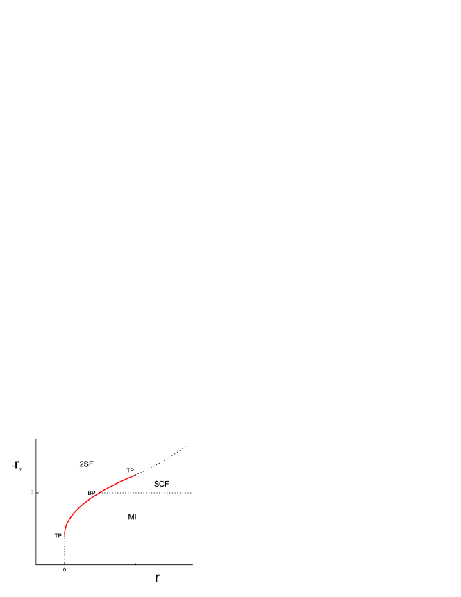
Figure 3: (Color online). Sketch of the mean field phase diagram for the effective action (3). The bold (red) solid line represents I-order transitions. Dotted lines are used for II-order transitions. The top of the solid line corresponds to upper TP, and the bottom – to lower TP. All three phase boundaries meet at BP.

It is worth stressing that the I-order transition is induced by fluctuations of the paired field $\Phi$. Indeed, one can approximately integrate $\Phi$ out using gaussian approximation for this field and generate an effective interaction term $\sim-(\gamma^{2}/|r_{m}|)|\psi_{1}|^{2}|\psi_{2}|^{2}$. It destabilizes the system for sufficiently small $|r_{m}|$ twocolor . Thus, the vicinity of BP must feature a I-order line (along MI-2SF and SCF-2SF). Correspondingly, there are two minimal values of $(\gamma^{2}/|r_{m}|)_{min}$ – one for $r_{m}>0$ and the other for $r_{m}<0$ – below which the transition becomes continuous along the respective boundaries. It is also important to realize that at the mean-field level there is no difference between the BH2 and DCP models.

Monte Carlo simulations twocolor did find an extended I-order MI-SF boundary and lower TP, but failed to resolve conclusively BP and upper TP. Standard numerical tools based on studies of hysteresis and probability distributions for the action were not precise enough for this system (close to TP the I-order transition is very weak and hard to identify in finite-size simulations). In all other respects, the mean field theory and simulations agreed on the topology of the phase diagram. Another important observation is that simulations of the same model (2) in $D=3+1$ dimensions unpubl revealed an extended region of first-order transitions above BP. Since $D=4$ is the upper critical dimension where fluctuations become essentially insignificant this result was expected. Thus, an intriguing possibility has emerged that the predicted first-order transition is destroyed by fluctuations in $D=2+1$.

In this work we apply a new flowgram method to perform a more refined analysis of the phase diagram in the vicinity of BP point and find that the SCF-SF boundary does contain a I-order region in $D=2+1$. The distance between BP and upper TP turns out to be an order of magnitude smaller than predicted by the mean-field theory. We attribute this to the fluctuation induced suppression of the pairing effect so that higher $V$ is required to produce the SCF phase.

At this point one may ask why not to trust the mean-field theory on another prediction, namely, the existence of lower TP for the DCP action. The precise answer lies in how the effective coefficients in (3) depend on $U,\,g$, and $L$. For the short-range model, the relation is rather straightforward, $\gamma\sim\sqrt{V}$, leading to finite value of lower TP at some $V=V_{LTP}\neq 0$. Ostensibly, the long-range nature of interaction in (1), which culminates in the runaway flow Halperin2 , makes the relation between $\gamma$ and $g$ system size dependent through $g_{\rm eff}=gL$ (in leading order in $g$) and precludes simple perturbative reasoning for lower TP even for small $g$. In other words, pairing correlations are never weak at large scales in the DCP action, and it is possible that this model is always above lower TP of the mean field theory (3).

III Flowgram method

In this Section we introduce the flowgram method and apply it to the study of the short-range model (2). The most fundamental property of current loops responsible for the superfluid response of the system are winding numbers Ceperley

$${\bf W}_{a}=L^{-1}\sum_{\bf r}{\bf j}_{a{\bf r}}\;.$$ (4)

Integer $W_{a}$ numbers count how many times ${\bf j}_{a{\bf r}}$ currents wind around the system with periodic boundary conditions. The superfluid stiffness, $\Lambda_{a}$, is directly proportional to $\langle{\bf W}_{a}^{2}\rangle/L$. For any scale-invariant transition there should be $\sim O(1)$ loops of size $R$ in a volume $R^{D}$, which implies that $\langle{\bf W}_{a}^{2}\rangle\sim O(1)$ at criticality and directly leads to the Josephson relation $\Lambda_{a}\sim 1/L$. Moreover, at the continuous transition point not only the $\langle{\bf W}_{a}^{2}\rangle$ value but also the whole distribution function $F({\bf W})$ is universal since it is governed by the system behavior at the largest scale.

Given close similarities between the DCP and BH2 phase diagrams it is convenient to introduce the following terminology: the transition line between phases with zero and non-zero ${\bf W}_{-}={\bf W}_{1}-{\bf W}_{2}$ winding number fluctuations is called a neutral line (described by proliferation of neutral  ${\bf j}_{-}={\bf j}_{1}-{\bf j}_{2}$ loops), and the transition line between phases with zero and non-zero ${\bf W}_{+}={\bf W}_{1}+{\bf W}_{2}$ winding number fluctuations is called a charged line (described by proliferation of charged  ${\bf j}_{+}={\bf j}_{1}+{\bf j}_{2}$ loops in addition to the loops of ${\bf j}_{-}$ which are already macroscopic). This terminology originates from the identification of $j$-currents as world line trajectories for charged spinon fields in the DCP action; only ${\bf j}_{+}$-currents are coupled by the long range Coulomb potential. Using this terminology, the SCF-SF (SFS-SF) transition is a charged line and the MI-SCF (VBS-SFS) transition is the neutral line; the two lines merge at BP. Notice that above BP the neutral winding number fluctuations $\langle{\bf W}^{2}_{-}\rangle$ on the charged line must exhibit linear growth with $L$ because the paired phase is characterized by finite stiffness (see Fig. 8). The same language will be used for the short-range action (2) even though no Coulomb potential is involved.

Formally, in Eq. (1) only ${\bf W}_{-}$ numbers may have non-zero values in the thermodynamic limit. Indeed, charged winding numbers couple to $Q_{{\bf q}=0}=1/q^{2}=\infty$ and thus are forbidden. However, charged loops of macroscopic size which simply do not wind around the system (but are similar to winding loops otherwise) are allowed and their contribution to the action can be estimated as $Q_{{\bf q}=1/L}/L\sim L$ (one would get the same result for loops with non-zero winding numbers if the zero-momentum compotent of the interaction potential is ”regularized”: $Q_{{\bf q}=0}\to Q_{{\bf q}=2\pi/L}\sim 1/L^{2}$). Since $Q_{{\bf q}=0}=\infty$ imposes a global constraint on a single variable of the configuration space of the model it may not have any effect on the nature of the scale-invariant transition. For example, on approach to the critical point charged loops of larger and large size (but smaller then $L\to\infty$ ) will proliferate anyway. We remove the global constraint by setting $Q_{{\bf q}=0}=Q_{{\bf q}=2\pi/L}$ for only one reason—to use non-zero winding number fluctuations as an indication of the deconfinement transition. We expect $\langle{\bf W}_{+}^{2}\rangle\sim 1$ at the transition point. The advantage of looking at the ${\bf W}_{+}$ numbers is that they are sensitive only to the deconfinement transition to the SF phase and remain zero in both the VBS and SFS phases.

The key elements of the flowgram method are:

• introduce a definition of the critical point for finite-size systems consistent with the thermodynamic limit and insensitive to the transition order,
  

• at the transition point, calculate quantities which are scale-invariant for the continuous phase transition in question, vanish in one of the phases and diverge in another; in our case such quantities are statistical averages of winding numbers squared, $R_{\mp}(L)=\langle{\bf W}_{\mp}^{2}\rangle$,
  

• study the flow of $R_{\mp}(L)$ with system size $L$ for given model parameters. As far as the thermodynamic critical points are concerned, the critical values of the corresponding parameters in the action are naturally obtained by extrapolating the sequence of finite-size critical points to $L=\infty$.

Observing how $R(L)$ scales with $L$ at the transition point allows studying the order of a transition, since $R(L\to\infty)$ has to saturate at some universal constant for second-order and to diverge for first-order transitions. Moreover, radical changes in the flowgram from saturation to divergence with an unstable separatrix in between as a function of coupling parameters is a clear sign of TP. It is important to emphasize that the flowgram method does not rely on detecting energy barriers between competing phases. It is simply based on phase coexistence typical for first-order transitions.

We use the following definition of a transition point: for any given set of $(g,L)$ or $(V,L)$ we determine the critical value of $U$ from the condition that the ratio of probabilities of having zero and non-zero winding numbers is some fixed number $C$ of the order of unity:

$$C_{+}=F(0)/\sum_{{\bf W}_{-}\neq 0}F({\bf W}_{-})=C\;,\quad C_{-}=F(0)/\sum_{{\bf W}_{+}\neq 0}F({\bf W}_{+})=C,$$ (5)

for the neutral and the charged lines, respectively. We use this particular criterion (among many others) because in the thermodynamic limit it gives exact answer for both second- and first-order transitions, since the ratio of probabilities in (5) is zero in the superfluid phase and infinity in the insulating phase note2 . As mentioned above, at the critical point we compute $R_{\pm}$. For the scale-invariant continuous transition one expects this quantity to approach its universal value as $L\to\infty$; for the the I-order transition it has to diverge with $L$ since in the superfluid phase $\langle{\bf W}_{\pm}^{2}\rangle\sim L$. The bicritical point is detected by observing vanishing charged winding numbers $R_{+}$ at the neutral line as $L$ is increased, and diverging, $R_{-}\propto L$, neutral winding numbers on the charged transition line.

Close to the weakly I-order transition the ratios $C_{\pm}$ (5) and averages $R_{\pm}$ exhibit strong fluctuations and are hard to compute precisely. However, fluctuations in $R_{\pm}$ are strongly correlated with fluctuations in $C_{\pm}$. This property, known as covariance, can be used to reduce statistical errors Sandvik2 . We have employed covariance, by plotting $R_{\pm}$ vs $C_{\pm}$, to reduce error bars by nearly an order of magnitude.

The flowgram method also allows to “visualize” the renormalization of coupling parameters. If data obtained for $(g_{1},L_{1})$ collapse on top of data for $(g_{2},L_{2})$ then one can consider this as an evidence that two systems are already in the scaling regime and are governed by the same effective coupling at large scales, $g_{\rm eff}(g_{1},L_{1})=g_{\rm eff}(g_{2},L_{2})$. In practice, we plot data for $R_{\mp}$ as a function of $\ln(L/\xi(g))$ where $\xi(g)$ is some interaction-dependent length-scale, i.e. we study if system properties at large scales are identical for different coupling constants $g$ up to the length-scale renormalization and are part of the same renormalization flow. If true, all data points for the DCP model should collapse on a single master curve. In the limit of small $g$, the runaway flow starts as $g_{\rm eff}(L)\propto gL$ Halperin2 , thus the length scale renormalization should follow the $\xi(g)\propto g^{-1}$ law.

III.1 Flowgrams for the short-range model

The most controversial region on the phase diagram for the BH2 model (2) is located in the vicinity of BP, see Fig. 2, where previous simulations failed to resolve the difference between BP and upper TP. The standard feature of I-order transitions – a double-peak shape of the probability distribution for energy/action $P(S)$ – works reliably only if there is a significant barrier between two phases. On approach to TP the barrier vanishes and the double-peak distribution method fails to work.

Using flowgrams one can identify the first-order transition even if no distinct discontinuity in system properties can be clearly seen. The cornerstone of the first-order transition is phase coexistence. In our case these phases are the insulator characterized by loops of small size (in the corresponding channel) and the superfluid in which the number of proliferated loops grows with the system size, so that the mean square winding number $\langle W^{2}\rangle\sim L$ for large enough sizes. The statistical properties of such mixture are drastically different from those of the second-order transition point characterized by scaling behavior, where the same number of loops of size $\sim L$ must be seen regardless of the (large) system size. The tricritical point is then characterized by the unstable separatrix separating the two limiting behaviors.

In Fig. 4, we show flows of $R_{+}$ vs $L$ for different values of $V$ along the MI-SF boundary. The separatrix position at $V=V_{LTP}\approx 0.5$ is consistent with lower TP found previously twocolor . In Fig. 5, the same separatrix is shown to be more pronounced in the neutral channel $R_{-}$. Below we will contrast these flows with the corresponding plots for the DCP action.

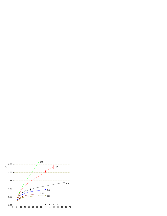
Figure 4: (Color online). Flowgrams for $R_{+}$ along the MI-SF line of the short-range model. The separatrix is located at lower TP given by $V=V_{LTP}\approx 0.5$.

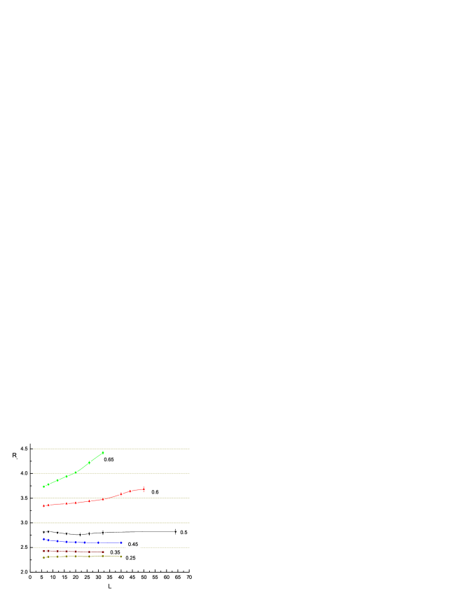
Figure 5: (Color online). Flowgrams for $R_{-}$ along the MI-SF line of the short-range model. The separatrix is located at lower TP given by $V=V_{LTP}\approx 0.5$.

Linear scaling $R_{+}\sim L$ is quite obvious close to upper TP as well, where no distinct double-peak probability distributions $P(S)$ were seen, see Fig. 6. As the interaction strength $V$ crosses the upper tricritical point located at $V_{UTP}\approx 0.925\pm 0.01$ the behavior changes from $R_{+}\sim L$ to $R_{+}\to const$.

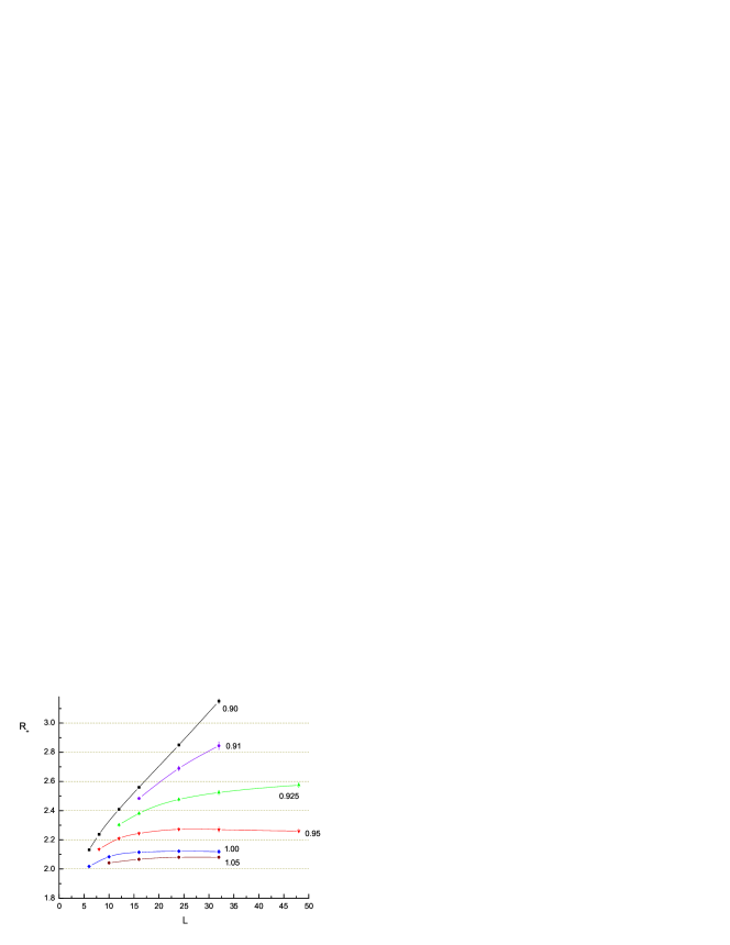
Figure 6: (Color online). Flowgrams for $R_{+}$ along the charged SCF-SF line of the short-range model. The upper tricritical point is identified from this plot to be at $V_{UTP}\approx 0.925$.

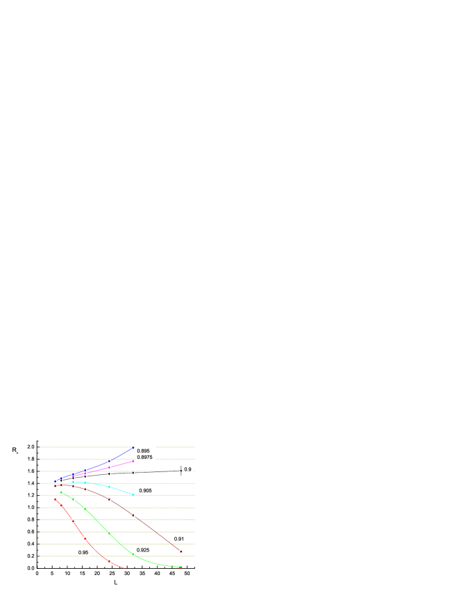
Figure 7: (Color online). Flowgrams for $R_{+}$ along the neutral MI-SCF line of the short-range model. The bicritical point is identified from this plot to be at $V_{BP}=0.90$.

Figure 8: (Color online). Flowgrams for $R_{-}$ along the charged MI-SF line of the short-range model in the SCF phase above the bicritical point ($V_{BP}=0.90$).

For the determination of BP, in Fig. 7 we present the flowgram of charged winding numbers on the neutral transition line close to the point where the MI-SF transition splits into two. For $V_{LTP}<V<V_{BP}=0.90\pm 0.005$ we observe diverging behavior typical for I-order transitions. For $V>V_{BP}$ the flow is towards zero values as $L$ increases and is indicative of the MI-SCF transition where only winding numbers in the neutral, or paired, channel proliferate. In contrast, the neutral windings $R_{-}$ diverge as $\sim L$ on the charged transition line (SCF-SF) because above the BP the SCF superfluid stiffness is finite in the SCF phase. This behavior is seen in Fig. 8.

Fig. 9 shows neutral winding numbers $R_{-}$ along the neutral line of MI-SCF transitions in the vicinity of BP. The crossover from linear scaling $R_{-}\propto L$ to saturation $R_{-}\to const$ is very sharp and is associated with passing through BP, where the II-order MI-SCF line terminates at the I-order MI-SF/SCF-SF line. From this plot we estimate $V_{BP}=0.90\pm 0.005$, in perfect agreement with the value deduced from flowgrams for the charged line, see Fig. 7.

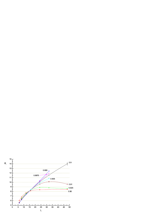
Figure 9: (Color online). Flowgrams for $R_{-}$ along the neutral MI-SCF line of the short-range model. This plot is consistent with the existence of BP at $V_{BP}=0.90$ (the same value was deduced from $R_{+}$ flowgrams) and I-order transitions at and slightly below $V_{BP}$.

Comparing $V_{BP}=0.90$ to $V_{UTP}=0.925$ we conclude that upper TP and BP do not coincide, and the actual phase diagram (see Fig. 18) is topologically identical to the mean field result twocolor . There is, however, a strong (about an order of magnitude) suppression of the I-order region above the BP due to strong fluctuation-induced corrections.

IV Deconfined Criticality

The field theory of DCP, built on fractionalized spinons (or vortices in the VBS phase), hints at the remarkable possibility of a generic continuous SF-VBS transition. Obviously, such II-order transition which occurs between phases characterized by different broken symmetries cannot be derived from the conventional Landau expansion in powers of the corresponding order parameter fields. One cannot even justify the perturbative expansion because it should start from the fully disordered quantum groundstate which has no broken symmetries (and topological orders). There are strong arguments that disordered quantum groundstate simply does not exist dcp3 ; weak1 . Another option is using a phenomenological Landau theory which combines superfluid and solid orders into one multi-component order parameter with non-zero modulus as a (non-perturbative) constraint YKIS ; weak1 . This approach, however, predicts that SF-solid transitions are generically of first-order with the exception of special high-symmetry points.

At first glance, DCP predictions are in sharp contradiction with the Landau approach. However, there is a fundamental difficulty in the DCP theory, namely, the runaway renormalization flow to strong coupling which makes the idea of generic continuous SF-VBS transition speculative and without reliable analytical support dcp3 . In the absence of stable perturbative fixed points other possibilities have to be explored as well. One alternative is that the DCP action is, in fact, a theory of generic I-order SF-VBS phase transitions (!) contrary to the original predictions. Early work on 3D scalar quantum electrodynamics Halperin2 did suggest that the renormalization flow leads to the I-order transition if the number of the matter-field components is relatively small ($\leq 100$). This prediction, however, is not taken seriously because it is known to be incorrect for the one-component system which, by the duality mapping Halperin , can be shown to have a continuous 3D XY transition. What happens in the multi-component case is a vast open problem in critical phenomena. It is worth noting, however, one aspect which is absent in the one-component case and becomes crucial in the case of two and more components —it is the presence of paired phases that may intervene between insulator and SF. Pairing effect was shown above to induce I-order superfluid-insulator transition for moderate coupling between components. Paring correlations in combination with the runaway flow to strong coupling Halperin2 would provide a natural explanation for the generic weakly I-order SF-VBS transitions in the DCP theory, as conjectured in Ref. YKIS .

The phase diagram for the DCP action shown in Fig. 2 is not specific to the $j-$current representation. A similar phase diagram is obtained for the XY phase-gauge field formulation of the theory Ref. Motrunich ; motrunich2 . More refined and extensive simulations have shown that early Monte Carlo results for the easy-plane model mentioned in Ref. Motrunich , section IIIA, did not go to sufficiently large system sizes to observe deviations from the power-law scaling and signatures of the weakly I-order transition motrunich2 . Since for $g\to 0$ the length scale for observing the I-order transition, if any, is guaranteed to diverge, one has to be extremely careful in monitoring deviations from the scaling behavior expected for the continuous scale-invariant transition. In Refs. Babaev ; Motrunich the second-order SF-VBS transition with the correlation length exponent $\nu\approx 0.6$ was deduced using straightforward power law fits of the data for system sizes $L\leq 24$. To make a point of comparison, we studied $\nu$ for the short-range model (BH2) along the SF-MI line for system sizes $L\leq 128$ using finite-size scaling of the superfluid density derivative, $\Lambda_{s}^{\prime}(U=U_{c})\propto L^{1/\nu-1}$. We found that (i) the scaling curves are nearly perfect straight lines on the log-log plot from the BP all the way to the lower TP, (ii) good scaling with $\nu\approx 0.4$ was observed up to $L=32$ in the middle of the I-order line(!), and (iii) in the upper half of the continuous $U(1)\times U(1)$ SF-MI line the slope of the best linear fit produced a set of interaction dependent $\nu(V)$ in the range between $0.67$ and $0.5$. This set of data is indicative of the fact that corrections to scaling are extremely important to take into account even for continuous transitions. With corrections to scaling included into the fits the data become consistent with $\nu\approx 0.67$ though the error bars increase by an order of magnitude. We thus conclude that for two-component models $\nu$ cannot be reliably determined on system sizes $L\leq 24$. More importantly, one may completely miss the I-order transition.

In what follows we discuss results of worm algorithm Monte Carlo simulations performed for the DCP action in the self-dual representation Babaev ; Motrunich (equivalent to the field theory of two identical scalar fields with Abelian gauge and U(1)$\times$U(1) symmetry of quartic interactions), construct its phase diagram, and prove our earlier assertion that the transition to the SF phase is always either I-order or through the SFS state YKIS . The supersolid state exists only for sufficiently large values of coupling to the gauge field $g>g_{BP}$ with $g_{BP}\approx 0.6$. For $g<g_{BP}$ we find I-order VBS-SF transition for any finite value of $g$.

IV.1 Bimodal distribution

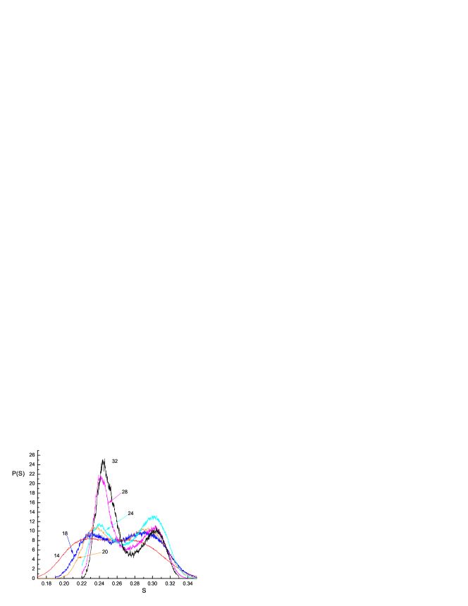
Figure 10: (Color online). Normalized probability density distributions $P(S)$ for the DCP action for $g=0.58$ and different system sizes; U(L=14)=1.0132, U(L=18)=1.0075, U(L=20)=1.0062, U(L=24)=1.0041, U(L=28)=1.00329, U(L=32)=1.00263.

Figure 11: Finite-size scaling of the peak positions in Fig. 10.

Before presenting flowgrams for the DCP action and interpreting them as evidence for the I-order deconfinement transition, we would like to discuss an unambiguous evidence of the I-order VBS-SF transition at $g=0.58$. The significance of this point will become clear shortly after we show that this point can be continuously related to smaller values of $g$ by the renormalization flow.

In the vicinity of the VBS-SF critical point defined according to the criterion (5) we look at the probability distribution $P(S)$ and finetune $U$ to the point where this distribution has the most pronounced double-peak structure or flat top. Unfortunately, simulations of large $L$ for the long-range action (1) are very time consuming, and $U$ has to be tuned with accuracy better then $10^{-4}$. Still, we were able to collect reliable statistics for system sizes $L\leq 32$, and have observed, see Fig. 10, the development of the double-peak structure in $P(S)$ starting from an anomalously flat maximum at $L=14$.

We are not aware of any continuous phase transition which features more and more pronounced double-peak distribution in energy/action with increasing the system size note1 , and consider Fig. 10 to be an unambiguous evidence in favor of the I-order transition. The scaling of peak positions with $L$ demonstrating no sign of peaks moving towards each other is presented in Fig. 11.

IV.2 Runaway flow and data collapse for small and intermidiate coupling

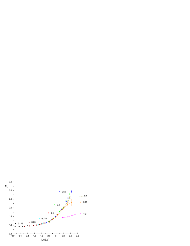
Figure 12: (Color online). Rescaled flowgrams for $R_{+}$ along the charged line. For $g<g_{BP}\approx 0.58$, this line coincides with the VBS-SF deconfinement transition, and, for $g>g_{BP}$, separates SF and SFS phases. System sizes are rescaled by $\xi=(g+g^{2})^{-1}$ so that the data for $g\leq 0.65$ collapse on a single master curve. The lines connect data points ($g>0.65$) which do not collapse.

In Fig. 12 we present the DCP action (1) flowgrams for various coupling constants $0.125\leq g\leq 1.2$ (the ending point $U=0$, $g\approx 1.6436$ corresponds to the inverted-XY transition along the charged line) and system sizes $8\leq L\leq 24$. We observe a remarkable data collapse by rescaling system sizes using $\xi(g)=(g+g^{2})^{-1}$ for values of $g$ up to $g=0.65$ (rescaling is equivalent to the horizontal shift of data points). The flow starts from the universal value corresponding to two decoupled $U(1)$ models and, most importantly, reaches the parameter range ($g=0.58$, $L\geq 14$) where we observe the development of the double-peak structure in $P(S)$. Several other features of the flow for $g<g_{BP}\approx 0.58$ are indicative of the I-order transition. We observe that $R_{-}$, Fig. 13, and $R_{+}$, Fig. 14, grow without saturation as expected for the mixture of superfluid and insulating phases. It cannot be reconciled with TP below $g_{BP}$ since TP implies an unstable separatrix and precludes data collapse.

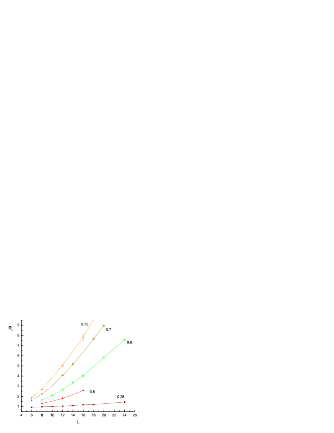
Figure 13: (Color online) Flowgrams for neutral winding numbers $R_{-}$ along the charged line demonstrating growth without saturation at all coupling constants. This behavior is drastically different from that observed in Fig. (5) for the short-range model, where the separatrix reveals lower TP.

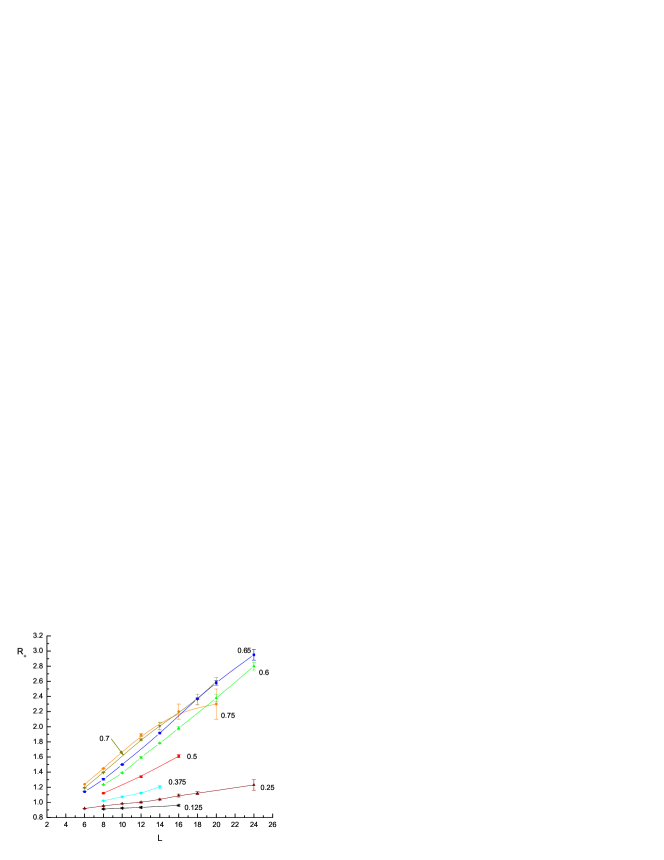
Figure 14: Flowgrams for charged winding numbers $R_{+}$ along the charged line. The same data as in Fig. 12 are now plotted without rescaling to underline linear divergence of $R_{-}$ with system size below $g_{UTP}\approx 0.70$.

As mentioned in the introduction, data collapse proves that systems with small $g$ and linear size $L$ have the same superfluid response as systems with larger $g$ and smaller $L$, i.e. their long-wave properties are governed by the renormalized coupling $g_{\rm eff}(g,L)$. We explicitly verify the perturbative renormalization group result $g_{\rm eff}\propto gL$ of Ref. Halperin2 for small $g$, and thus exclude any possibility for having TP at $g<0.125$. Renormalization procedure allows us to extend the flowgram to sufficiently large values of $gL>18$ and to relate systems with arbitrary small $g$ to the first-order transition because data points for $g=0.58$ are collapsing on the same continuous curve. [Simulating $gL=18$ for $g=0.125$ would be equivalent to having $L=115$ – an impossible task for the long-range model.] Thus, we conclude that the I-order transition line goes all the way to the special $g=0$ point which is described by the $U(1)\times U(1)$ universality for two independent complex scalar fields

IV.3 Flowgrams along the charged line (SFS-SF transition)

For $g>0.65$ the flow collapse starts to break down. This region features BP and upper TP; for $g>0.8$ the presence of the paired SFS phase can be seen by the flowgram method even in small samples. The flow collapse on the charged line fails because the order of the transition changes at upper TP ( we estimate $g_{UTP}=0.70\pm 0.05$) which features an unstable separatrix. For $g>g_{UTP}$ we are dealing with the continuous SF-SFS transition of the inverted-XY type. The diverging flow, then, is replaced with saturation clearly seen already for $g=0.75$.

In Fig. 13 we present data for flowgrams of neutral winding numbers along the same (charged) line. This time we do not rescale distances to verify that $R_{-}$ obeys the linear law $R_{-}\propto L$ characteristic of finite superfluid response in the SFS and SF phases, or phase coexistence at the I-order transition. The divergent flow observed for $R_{-}$ at all $g$ on the charged line by itself is suggesting that BP (where the I-order SF-VBS line splits into SCF-SF and SCF-VBS lines) is below $g_{UTP}\approx 0.70$: otherwise, we would observe saturation of $R_{-}$ between the two milticritical points. Linear scaling of $R_{+}$ for $g<g_{UTP}$ is presented in Fig. 14

IV.4 Flowgrams along the neutral line (VBS-SFS transition)

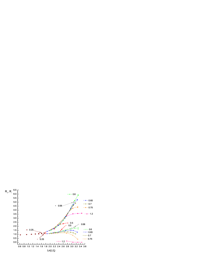
Figure 15: Renormalized flowgrams of $R_{\pm}$ along the neutral line. For $g<g_{BP}\approx 0.58$ this line coincides with the I-order VBS-SF deconfinement transition and for $g>g_{BP}$ it separates SFS and VBS phases. Each symbol corresponds to a value of $g$ shown. The upper set of data points is for neutral winding numbers $R_{-}$ (solid symbols), and the lower set is for charged ones $R_{+}$ (open symbols). The lines connect data points ($g\geq 0.58$) which do not collapse on the master curve.

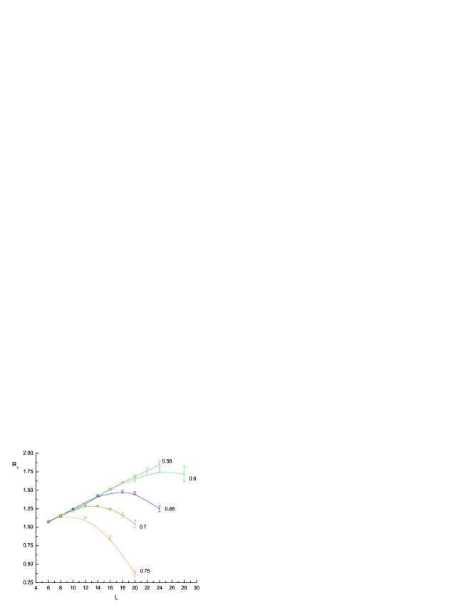
Figure 16: Flowgrams for charged winding numbers $R_{+}$ along the neutral line.

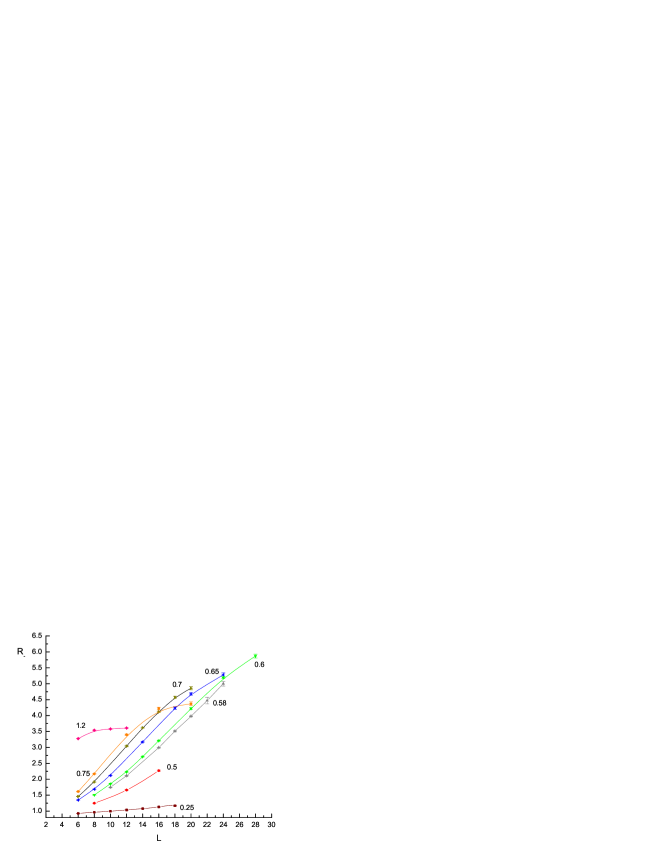
Figure 17: Flowgrams for neutral winding numbers $R_{-}$ along the neutral line for $g>g_{BP}\approx 0.58$ and along the VBS-SF transition for $g<g_{BP}$.The latter set of the points exhibits linear growth due to the I-order transition as in Fig. (13).

Though flowgrams for the charged transition line are sufficient to determine the topology of the phase diagram, they are rather insensitive to the location of BP. Instead, one has to look at flowgrams for the neutral line to observe how it branches out from the I-order SF-VBS line. These are shown in Fig. 15. A nearly perfect data collapse on divergent flow is observed for both types of winding numbers up to $g\approx g_{BP}\approx 0.58\pm 0.02$. In Figs. 16 and 17 the same data are plotted without rescaling to underline linear divergence of $R_{\pm}$ with system size below BP. For higher values of $g$, winding numbers in the charged channel start decaying to zero and the flow cannot be collapsed any more. This is an unambiguous sign that we have passed BP and the neutral SFS-VBS line has branched out from the I-order VBS-SF transition. At the same time, though less dramatically, the neutral winding numbers turn to saturation, as expected for the continuous XY transition.

Figure 18: (Color online). Fine structure of phase diagrams for the long-range (left panel), Eq. (1), and short-range (right panel), Eq. (2), actions in the vicinity of BP. Bold solid lines indicate the I-order phase transition.

We summarize our results for the phase diagrams of the DCP and BH2 actions in Fig. 18 which is showing fine details invisible in Fig. 2. One may not miss that SF-SFS and SFS-VBS lines go extremely close to each other between upper TP and BP. It is only due to the flowgram method that we were able to resolve them conclusively. The most important result we learn from Fig. 18 is that pairing fluctuations, at the qualitative level correctly captured by the mean-field theory, always place the BP below the upper TP regardless of the interaction range.

V Conclusion

To conclude, we have shown that the runaway renormalization flow to strong coupling in the U(1)$\times$U(1) symmetric two-component scalar quantum electrodynamics in $D=2+1$ leads to a I-order deconfinement transition to the SF state. This result, and the structure of the phase diagram for relatively strong coupling between the spinons exclude the possibility of generic continuous VBS-SF transition in the self-dual deconfined critical action. The I-order transition is fluctuation induced—it develops at progressively larger length scales as $g\to 0$.

Though in this work we considered a particular DCP model, Eq. (1), our results have a certain degree of universality since the I-order transition was found to be very weak and fully developed only in large systems with more than $10^{4}$ sites (all results for small $g$ are universal since they are subject to the renormalization flow). Thus, our study does rule out the possibility of having continuous VBS-SF transitions in models with weak-to-intermediate long-range coupling. Yet one may argue that our simulations do not rule the possibility of continuous VBS-SF transition in some part of the phase diagram of some yet unexplored model, say, for large couplings. Of course, they do not. But there is no evidence or even good theoretical argument that such a transition line will not be eliminated by the tendency to pairing at large $g$. Such model, if any, would rather be an exception; the generic situation is that the combination of the runaway flow and pairing correlations drives a system into either the first-order transition for weak and intermediate couplings or to the paired phase for large ones. At the phenomenological level, we think that the strongest argument against DCP is Landau theory based on the multi-component order parameter with non-zero modulus—so far, all numerical data for various microscopic models of the VBS-SF transition are consistent with it.

We are grateful to E. Vicari, O. Motrunich, S. Sachdev, M. Fisher, T. Senthil, A. Vishvanath, Z. Tešanović for valuable and stimulating discussions. The research was supported by the National Science Foundation under Grants No. PHY-0426881 and PHY-0426814, the PSC CUNY Grant No. 665560036, and by the Swiss National Science Foundation. The CUNY Supercomputer Grid, in general, and the CSI Linux Supercomputer Cluster, in particular, played an important role in the project. We also acknowledge hospitality of the Aspen Center for Physics during the Summer 2005 Workshop on Ultracold Atoms.

References

- (1) B.I. Halperin, T.C. Lubensky, and S.-K. Ma, Phys. Rev. Lett. 32, 292 (1974).
- (2) E. Brzin, J.C. Le Guillou, and J. Zinn-Justin, Phys. Rev. B 10, 892 (1974).
- (3) J.-H. Chen, T.C. Lubensky, and D. Nelson, Phys. Rev. B 17, 4274 (1978).
- (4) E. Babaev, Nucl. Phys. B 686, 397 (2004); J. Smiseth, E. Smørgrav, E. Babaev, and A. Sudbø, cond-mat/0411761.
- (5) T. Senthil,A. Vishwanath, L. Balents, S. Sachdev, and M.P.A. Fisher, Science 303, 1490 (2004).
- (6) T. Senthil, L. Balents, S. Sachdev, A. Vishwanath, and M.P.A. Fisher, Phys. Rev. B 70 144407 (2004).
- (7) L. Balents, L. Bartosch, A. Burkov, S. Sachdev, and K. Sengupta Phys. Rev. B 71 144509 (2005); ibid 144508 (2005).
- (8) S. Coleman and E. Weinberg, Phys. Rev. D 7, 1988 (1973).
- (9) O.I. Motrunich and A. Vishwanath, Phys. Rev. B 70, 075104 (2004).
- (10) H. P. Büchler, M. Hermele, S. D. Huber, M. P. A. Fisher, and P. Zoller, Phys. Rev. Lett. 95, 040402 (2005).
- (11) A.B. Kuklov, N.V. Prokof’ev, and B.V. Svistunov, Phys. Rev. Lett. 92, 050402 (2004).
- (12) A.B. Kuklov and B.V. Svistunov, Phys. Rev. Lett. 90, 100401 (2003).
- (13) A.B. Kuklov, N.V. Prokof’ev, and B.V. Svistunov, to be published in Prog. Theor. Phys. Japan, 160 (2005).
- (14) K. Binder, Phys. Rev. Lett. 47, 693 (1981); K. Binder, D.P. Landau, A Guide to Monte Carlo Simulations in Statistical Physics (Cambridge University Press, Cambridge, 2000).
- (15) R.G. Melko, A.W. Sandvik, and D.J. Scalapino, Phys. Rev. B 69, 100408(R) (2004); private communications.
- (16) A. Kuklov, N. Prokof’ev, and B. Svistunov, Phys. Rev. Lett. 93, 230402 (2004).
- (17) A.B. Kuklov, N.V. Prokof’ev, and B.V. Svistunov, unpublished.
- (18) E.I. Pollock and D.M. Ceperley, Phys. Rev. B 36, 8343 (1987).
- (19) Obviously, a choice of determines only how fast the thermodynamic limit is reached. For the DCP and the BH2 models we used and , respectively. These values are close to at the critical point of the XY-model. We verified that changing within the range from unity to about 10 does not change the qualitative features of the flowgrams.
- (20) A.W. Sandvik, Phys. Rev. B 54, 5334 (1996).
- (21) M. Peskin, Ann. Phys. 113 (1978); P.R. Thomas and M. Stone, Nucl. Phys. B 144, 513 (1978); C. Dasgupta and B.I. Halperin, Phys. Rev. Lett. 47, 1556 (1981).
- (22) O.I. Motrunich, private communication.
- (23) In certain models of continuous phase transitions the double peak distribution is observed for small system sizes but it evolves into the single-peak distribution for large .