Diagrammatic analysis of correlations in polymer fluids: Cluster diagrams via Edwards’ field theory

Abstract

Edwards’ functional integral approach to the statistical mechanics of polymer liquids is amenable to a diagrammatic analysis in which free energies and correlation functions are expanded as infinite sums of Feynman diagrams. This analysis is shown to lead naturally to a perturbative cluster expansion that is closely related to the Mayer cluster expansion developed for molecular liquids by Chandler and coworkers. Expansion of the functional integral representation of the grand-canonical partition function yields a perturbation theory in which all quantities of interest are expressed as functionals of a monomer-monomer pair potential, as functionals of intramolecular correlation functions of non-interacting molecules, and as functions of molecular activities. In different variants of the theory, the pair potential may be either a bare or a screened potential. A series of topological reductions yields a renormalized diagrammatic expansion in which collective correlation functions are instead expressed diagrammatically as functionals of the true single-molecule correlation functions in the interacting fluid, and as functions of molecular number density. Similar renormalized expansions are also obtained for a collective Ornstein-Zernicke direct correlation function, and for intramolecular correlation functions. A concise discussion is given of the corresponding Mayer cluster expansion, and of the relationship between the Mayer and perturbative cluster expansions for liquids of flexible molecules. The application of the perturbative cluster expansion to coarse-grained models of dense multi-component polymer liquids is discussed, and a justification is given for the use of a loop expansion. As an example, the formalism is used to derive a new expression for the wave-number dependent direct correlation function and recover known expressions for the intramolecular two-point correlation function to first order in a renormalized loop expansion for coarse-grained models of binary homopolymer blends and diblock copolymer melts.

1 Introduction

Diagrammatic expansions have played an important role in the development of the theory of classical fluids. They have proved useful both as a tool for the development of systematic expansions in particular limits, and as a language for the analysis of proposed approximation schemes. Analysis of Mayer cluster expansions of properties of simple atomic liquids was brought to a very high degree of sophistication by the mid-1960s [1, 2, 3]. Corresponding Mayer cluster expansions were later developed for interaction site models of both rigid [4] and non-rigid molecules [5, 6, 7] by Chandler and coworkers. Throughout, the development of both atomic and molecular liquid state theory has been characterized by an interplay between diagrammatic analysis [8, 9] and the development of integral equation approximations [10, 11, 12, 13, 14, 15, 16].

A field-theoretic approach that was introduced by Edwards [17, 18] has been used in many studies of coarse-grained models of polymer liquids. Edwards’ approach relies upon an exact transformation of the partition function of a polymer fluid from an integral with respect to monomer positions to a functional integral of a fluctuating chemical potential field. A saddle-point approximation to this integral leads [19] to a simple form of mean field theory, which further reduces to a form of Flory-Huggins theory in the case of a homogenous mixture. The first applications of this approach were studies of excluded volume effects polymer solutions, by Edwards, Freed, and Muthukumar [17, 18, 19, 20, 21, 22]. Several authors have since used Edwards’ formalism to study corrections to mean field theory in binary homopolymer blends and in block copolymer melts [24, 25, 26, 27, 28, 29, 30, 31, 32, 33, 34, 35]. All of these studies of dense liquids have been based upon some form of Gaussian, or, equivalently [23], one-loop approximation for fluctuations about the mean field saddle-point. This formalism is also the basis of a numerical simulation method developed by Fredrickson and coworkers [36, 37], in which the functional integral representation of the partition function is sampled stochastically.

Edwards’ approach lends itself to the use of standard methods of perturbative field theory, including the use of Feynman diagrams. By analogy to experience with both Mayer cluster expansions in the theory of simple liquids, and of Feynman diagram expansions in statistical and quantum field theories, one might expect it to be possible to develop systematic rules for the expansion of the free energy and various correlation functions as well-defined infinite sets of Feynman diagrams. Such rules have, however, never been developed for Edwards’ field-theoretic approach with a level of generality or rigor comparable to that attained long ago for either Mayer clusters or statistical field theory. This paper attempts to rectify this, while also exploring connections between different diagrammatic approaches to liquid state theory.

The analysis given here starts from a rather generic interaction site model of a fluid of non-rigid molecules. Molecules are comprised of point-like particles (referred to here as “monomers” ) that interact via a pairwise additive two-body interaction, and via an unspecified intramolecular potential among monomers within each molecule. The diagrammatic expansion that is obtained by applying the machinery of perturbative field theory to a functional integral representation of the grand partition function is a form cluster expansion, which is referred to here as an interaction site perturbative cluster expansion. Terms in this expansion are conveniently represented in terms of diagrams of bonds and vertices, in which vertices represent multi-point intramolecular correlation functions. In different variants of the theory, the bonds may represent either the screened interaction identified by Edwards [17, 18] or the bare pair potential.

The expansion in terms of the bare potential is shown to be a particularly close relative of the interaction site Mayer cluster expansion developed for fluids of non-rigid molecules by Chandler and Pratt [5]. The main differences are differences in the diagrammatic rules that arise directly from the association of a factor of the pair potential rather than the corresponding Mayer $f$-function with each bond. A self-contained derivation of the Chandler-Pratt Mayer cluster expansion for a molecular liquid is given in Sec. 22. The derivation of the Mayer cluster expansion given here follows a line of reasoning closely analogous to that used in the theory of simple liquids, which starts from an expansion of the grand-canonical partition function. The derivation is somewhat more general and (arguably) more direct than that given by Chandler and Pratt.

One result of the present analysis that does not seem to have an analog in the Mayer cluster analysis of Chandler and Pratt is an expansion of a generalized Ornstein-Zernicke direct correlation function for a fluid of flexible molecules. This is presented in Sec. 17.

Throughout, the analyses of both perturbative and Mayer cluster expansions proceed by reasoning that is, as much as possible, analogous to that given for atomic liquids by Morita and Hiroike [1], Stell [2], and Hansen and MacDonald [3]. Diagrammatic rules for the calculation of correlation functions are derived by functional differentiation of an expansion of a grand canonical thermodynamic potential with respect to fields conjugate to monomer concentrations. Several renormalized expansions are obtained by topologically reductions roughly analogous to those applied previously to atomic fluids. Because the diagrams used to construct perturbative cluster expansions for fluids of non-rigid molecules are different than those used in either the Mayer cluster expansion for atomic liquids or in other applications of statistical field theory, the main text is supplemented by a discussion in appendices C and D of the symmetry numbers needed to calculate combinatorical prefactors for such diagrams, and in appendices E and F by several lemmas about diagrams that are needed to justify various topological reductions. The required lemmas are all generalizations of those given by Morita and Hiroike for fluids of point particles.

Once the close relationship between the perturbative and Mayer cluster expansions is appreciated, it reasonably to ask for what classes of problems a perturbative expansion might be useful. A perturbative description of a classical fluid is useful only for models with relatively soft or long-range pair interactions. It is thus clearly not a useful starting point for treating the harsh repulsive interactions encountered in any atomistic model of a dense liquid. As discussed in Sec. 19, a perturbative expansion is, however, potentially useful for the study of very coarse-grained models of dense multi-component polymer liquids [35]. In such models, in which each monomer is a soft “blob” that represents a subchain of many chemical monomers, the effective interaction between blobs is much softer and of much longer range than the interactions between atoms or chemical monomers. It is shown here that a loop expansion of the perturbative diagrammatic expansion for such a model yields an asymptotic expansion about the mean field theory when the coarse-grained monomers are taken to be large enough so as to strongly overlap. The small parameter in this expansion is the ratio of the packing length of the melt (which is independent of the degree of coarse-graining) to the size of a coarse-grained monomer.

As an example, in Sec. 20 the formalism is used to derive expressions for the two-point intramolecular correlation function and the direct correlation function in both binary homopolymer mixtures and block copolymer melts to first order in a renormalized loop expansion. The resulting expressions are compared to those obtained by related methods in several previous studies.

Notwithstanding its title, very little in this article is specific to high molecular weight polymers: All of the results, except those of Sec. 19, are formally applicable to any interaction site model of a classical fluid of non-rigid molecules. The analysis is nonetheless reasonably described as a theory of polymer liquids both for sociological reasons, because Edwards’ approach has been used primarily by polymer physicists for the study of coarse-grained models of polymer liquids, and for practical reasons, because this approach seems to be best suited for this purpose.

2 Model and Definitions

We consider a mixture of $S$ molecular species, each of which is constructed from a palette of $C$ types of monomer. Each molecule of species $a$, where $a=1,\ldots,S$, contains $N_{ai}$ monomers of type $i$, where $i=1,\ldots,C$. The total number of molecules of type $a$ is $M_{a}$ in a system of volume $V$, giving a number density $\rho_{a}\equiv\langle M_{a}\rangle/V$. The following conventions are used throughout for the names and ranges of indices:

$$\begin{array}[]{rcll}a,b&=&1,\ldots,S&{\rm molecule\ species}\\ i,j&=&1,\ldots,C&{\rm monomer\ types}\\ m&=&1,\ldots,M_{a}&{\rm molecules}\\ s&=&1,\ldots,N_{ai}&{\rm monomer\ sites}\end{array}$$ (1)

Unless otherwise stated, summations over indices are taken over the ranges indicated above, and summation over repeated indices is implicit.

Let ${\bf R}_{ami}(s)$ be the position of monomer $s$ of type $i$ on molecule $m$ of species $a$. We define monomer density fields

$$c_{ami}({\bf r}) \equiv \sum_{s}\delta({\bf r}-{\bf R}_{ami}(s))$$

$$c_{i}({\bf r}) \equiv \sum_{am}c_{ami}({\bf r})\;\;.$$ (2)

These give the number concentrations for monomers of type $i$ on a specified molecule $m$ of type $a$, and for all monomers of type $i$, respectively.

2.1 Model

We consider a class of models in which the total potential energy of a molecular liquid is given by a sum

$$U=U_{0}+U_{int}+U_{ext}\;\;.$$ (3)

Here, $U_{0}$ is an intramolecular potential energy. This might be taken to be a Gaussian stretching energy in a coarse-grained model of a polymer chain, but its exact form may be left unspecified. The energy $U_{int}$ is a pairwise-additive interaction between monomers, of the form

$$U_{int}\equiv\frac{1}{2}\sum_{ij}\int\!d{\bf r}\int\!d{\bf r}^{\prime}\;U_{ij}({\bf r}-{\bf r}^{\prime})c_{i}({\bf r})c_{j}({\bf r}^{\prime})$$ (4)

in which $U_{ij}({\bf r}-{\bf r}^{\prime})$ is the interaction potential for monomers of types $i$ and $j$. The external potential is of the form

$$U_{ext}=-\sum_{i}\int\!d{\bf r}\;h_{i}({\bf r})c_{i}({\bf r})\;\;,$$ (5)

where $h_{i}({\bf r})$ is an external field conjugate to $c_{i}({\bf r})$. The external field $h$ is introduced solely as a mathematical convenience, so that expressions for correlation functions may be derived by functional differentiation of the grand potential with respect to $h$.

The canonical partition function for a system with a specified number $M_{a}$ of molecules of each type $a$, as a functional of the multi-component field $h$, is denoted

$$Z_{\underline{M}}[h]=\frac{1}{M_{1}!\cdots M_{C}!}\int\!D[{\bf R}]\;e^{-U}\;\;,$$ (6)

where $\underline{M}$ denotes a set of values $\underline{M}=\{M_{1},\ldots,M_{C}\}$ for all species, and $D[{\bf R}]$ denotes an integral over the positions of all monomers in the system. Here and hereafter, we use units in which $k_{B}T\equiv 1$. The grand-canonical partition function is

$$\Xi\equiv\sum_{\underline{M}}e^{\mu_{a}M_{a}}Z_{\underline{M}}[h]={\rm Tr}[e^{-U+\mu_{a}M_{a}}]$$ (7)

where $\mu_{a}$ is a chemical potential for molecular species $a$, which corresponds to an activity $\lambda_{a}\equiv e^{\mu_{a}}$, and $\sum_{\underline{M}}$ denotes a sum over $M_{a}\geq 0$ for all $a$. The second equality in Eq. (7) introduces the notation ${\rm Tr}[\cdots]$ to represent integration over all distinguishable sets of monomer positions and summation over $M_{a}$.

2.2 Notational Conventions

Functions of $n$ monomer positions and $n$ corresponding monomer type indices may be expressed either using a notation

$$F_{\underline{i}}(\underline{\bf r})\equiv F_{i_{1}\cdots i_{n}}({\bf r}_{1},\ldots,{\bf r}_{n})$$ (8)

in which $\underline{i}\equiv\{i_{1},i_{2},\ldots,i_{n}\}$ and $\underline{\bf r}\equiv\{{\bf r}_{1},{\bf r}_{2},\ldots,{\bf r}_{n}\}$ denote lists of monomer type and positions arguments, respectively, or in an alternative notation

$$F(1,\ldots,n)\equiv F_{i_{1}\cdots i_{n}}({\bf r}_{1},\ldots,{\bf r}_{n})$$ (9)

in which an integer argument ‘$j$’ represents both a position ${\bf r}_{j}$ and a monomer type index $i_{j}$.

The notation $H=G*F$, when applied to two-point functions, represents a convolution

$$H(1,3)=\int d(2)\;G(1,2)F(2,3)$$ (10)

in which $\int d(j)\equiv\sum_{j}\int\!d{\bf r}_{j}$ denotes both integration over a coordinate ${\bf r}_{j}$ and summation over the corresponding type index. Similarly, $h*c$ is shorthand for an integral $\int d(1)h(1)c(1)$. The function $F_{ij}^{-1}({\bf r},{\bf r}^{\prime})$ denotes the integral operator inverse of a two-point function $F_{ij}({\bf r},{\bf r}^{\prime})$, which is defined by an integral equation by $F*F^{-1}=\delta$ where $\delta(1,3)\equiv\delta_{i_{1}i_{3}}\delta({\bf r}_{1}-{\bf r}_{3})$.

Coordinate-space and Fourier representations of functions of several variables may be used essentially interchangeably in most formal relationships. Fourier transforms of fields such as the monomer density $c_{i}({\bf r})$ are defined with the convention $c_{i}({\bf k})\equiv\int\!d{\bf r}\;e^{-i{\bf k}\cdot{\bf r}}c_{i}({\bf r})$, while transforms of functions of two or more monomer positions and type indices, such as $U_{ij}({\bf r}_{1},{\bf r}_{2})$, are defined with the convention

$$F_{\underline{i}}(\underline{\bf k})\equiv\frac{1}{V}\int d^{n}{\bf r}\;e^{-i{\bf k}_{j}\cdot{\bf r}_{j}}F_{\underline{i}}(\underline{\bf r})$$ (11)

where $\int d^{n}{\bf r}=\int\!d{\bf r}_{1}\cdots\int\!d{\bf r}_{n}$, and where $\underline{\bf k}\equiv\{{\bf k}_{1},{\bf k}_{2},\ldots,{\bf k}_{n}\}$ denotes a list of $n$ wavevector arguments. The prefactor of $1/V$ in Eq. (11) guarantees that the transform $F_{\underline{i}}(\underline{\bf k})$ of a translationally invariant function will approach a finite limit as $V\rightarrow\infty$ if ${\bf k}_{1}+{\bf k}_{2}+\cdots+{\bf k}_{n}=0$ (and must vanish otherwise). When this convention matters, an $n$-point function $F_{\underline{i}}(\underline{\bf k})$ defined by convention (11) will be referred to as a normalized Fourier transform of $F_{\underline{i}}(\underline{\bf r})$, and $VF_{\underline{i}}(\underline{\bf k})$ as the unnormalized transform. The normalized transform of a translationally invariant two-point function, such as $U_{ij}({\bf r}-{\bf r}^{\prime})$, may be expressed as a function $U_{ij}({\bf k})\equiv U_{ij}({\bf k},-{\bf k})$ of only one wavevector. The normalized transform $F_{ij}^{-1}({\bf k})\equiv F_{ij}^{-1}({\bf k},{\bf k}^{\prime})$ of the inverse of a translationally invariant function $F$ is simply the matrix inverse of $F_{ij}({\bf k})$.

2.3 Collective Correlation and Cluster Functions

An $n$-point correlation function $R^{(n)}$ of the collective monomer density fields is given by the expectation value

$$R^{(n)}_{\underline{i}}(\underline{\bf r}) \equiv \langle c_{i_{1}}({\bf r}_{1})c_{i_{2}}({\bf r}_{2})\cdots c_{i_{n}}({\bf r}_{n})\rangle$$ (12)

$$= \frac{1}{\Xi}\frac{\delta^{n}\Xi}{\delta h_{i_{1}}({\bf r}_{1})\cdots\delta h_{i_{n}}({\bf r}_{n})}$$

or, in more compact notation,

$$R^{(n)}(1,\ldots,n) \equiv \langle c(1)c(2)\cdots c(n)\rangle$$ (13)

$$= \frac{1}{\Xi}\frac{\delta^{n}\Xi}{\delta h(1)\cdots\delta h(n)}$$

where $c(j)\equiv c_{i_{j}}({\bf r}_{j})$.

Collective cluster functions are related to the correlation functions by a cumulant expansion. Collective cluster functions are defined, in compact notation, as

$$S^{(n)}(1,\ldots,n) \equiv \langle c(1)c(2)\cdots c(n)\rangle_{c}$$ (14)

$$= \frac{\delta^{n}\ln\Xi}{\delta h(1)\cdots\delta h(n)}$$

where the notation $\langle\cdots\rangle_{c}$ denotes a cumulant of the product of variables between angle brackets. For example, the two-point cluster function is given by the cumulant $S(1,2)\equiv\langle c(1)c(2)\rangle-\langle c(1)\rangle\langle c(2)\rangle$, also referred to as the structure function.

2.4 Intramolecular Correlation Functions

The intramolecular correlation function

$$\Omega_{a,\underline{i}}^{(n)}(\underline{\bf r})\equiv\langle\sum_{m=1}^{M_{a}}c_{ami_{1}}({\bf r}_{1})\cdots c_{ami_{n}}({\bf r}_{n})\rangle$$ (15)

describes correlations among monomers that are part of the same molecule $m$ of species $a$. In more compact notation,

$$\Omega_{a}^{(n)}(1,\ldots,n)\equiv\langle\sum_{m=1}^{M_{a}}c_{am}(1)\cdots c_{am}(n)\rangle\;\;,$$ (16)

where $c_{am}(j)=c_{ami_{j}}({\bf r}_{j})$. We also define a function

$$\Omega^{(n)}(1,\ldots,n)\equiv\sum_{a}\Omega_{a}^{(n)}(1,\ldots,n)\;\;.$$ (17)

The sum in Eq. (17) must be taken only over species of molecule that contain monomers of all types specified in the argument list $\underline{i}=\{i_{1},\ldots,i_{n}\}$, since $\Omega_{a,\underline{i}}^{(n)}(\underline{\bf r})=0$ otherwise. Note that the single-species correlation function $\Omega_{a}(1,\ldots,n)$ and the sum $\Omega^{(n)}(1,\ldots,n)$ defined in Eq. (17) are distinguished typographically only by the presence or absence of a species index $a$.

The value of $\Omega_{a}^{(n)}(1,\ldots,n)$ for a specified set of arguments is roughly proportional to the number density $\rho_{a}\equiv\langle M_{a}\rangle/V$ for molecules of type $a$, and vanishes as $\rho_{a}\rightarrow 0$. To account for this trivial concentration dependence, we also define a single-molecule correlation function

$$\omega_{a}^{(n)}(1,\ldots,n)\equiv\Omega_{a}^{(n)}(1,\ldots,n)/\rho_{a}\quad.$$ (18)

The normalized Fourier transform $\omega_{a,\underline{i}}^{(n)}(\underline{\bf k})$ may be expressed as an average

$$\omega_{a,\underline{i}}^{(n)}(\underline{\bf k})=\sum_{s_{1},\cdots,s_{n}}\left\langle e^{i\sum_{j}{\bf k}_{j}\cdot{\bf R}_{ami}(s_{j})}\right\rangle$$ (19)

for an arbitrarily chosen molecule $m$ of type $a$.

For example, in a homogeneous liquid containing Gaussian homopolymers of type $a$, each containing $N$ monomers of type $i$ and statistical segment length $b$, $\omega_{a,ii}^{(2)}({\bf k})=N^{2}_{a}g(k^{2}N_{a}b^{2}_{i}/6)$, where $g(x)\equiv 2[e^{-x}-1+x]/x^{2}$ is the Debye function. In the limit ${\bf k}\rightarrow 0$, this quantity approaches $\omega_{a,ii}^{(2)}(0)=N^{2}_{a}$. In a liquid containing block copolymers of species $a$, the function $\omega_{a,ij}^{(2)}({\bf k})$ describes correlations between monomers in blocks $i$ and $j$.

2.5 Direct Correlation Function

We define a collective direct correlation function $C(1,2)$ for monomers of type $i$ and $j$ in a homogeneous fluid by a generalized Ornstein-Zernicke (OZ) relation

$$S^{-1}(1,2)=\Omega^{-1}(1,2)-C(1,2)\;\;,$$ (20)

or $S^{-1}_{ij}({\bf k})=\Omega^{-1}_{ij}({\bf k})-C_{ij}({\bf k})$ in a homogeneous liquid, in which $\Omega^{-1}$ is the inverse of the two-point intramolecular correlation function $\Omega^{(2)}$ defined in Eq. (17). The random phase approximation (RPA) for $S^{-1}$ in a compressible liquid is obtained by approximating $-C$ by the bare potential $U$.

The definition of a monomer “type” used here is somewhat flexible. Because all monomers of the same type $i$ are assumed in Eq. (4) to have the same pair potential $U_{ij}$ with all monomers of type $j$, monomers of the same type must be chemically identical. It is sometimes useful, however, to divide sets of chemically identical monomers into subsets that are treated formally as different types. For example, it may be useful for some purposes to define each “type” of monomer to include only monomers of a given chemical type on a specific molecular species. If we go further, and take each monomer “type” $i$ to include only monomers that occupy a specific site $s$ on a specific species of molecule $a$, then generalized Ornstein-Zernicke equation (20) becomes equivalent to the site-site OZ equation used in reference interaction site model (RISM) integral equation theories, [10, 11, 12, 13, 14, 15, 16] and $C(1,2)$ to the corresponding site-site direct correlation function.

2.6 Thermodynamic Potentials

The grand canonical thermodynamic potential $\Phi$ and Helmholtz free energy $A$ are given by

$$\Phi(\mu;[h]) \equiv -\ln\Xi$$ (21)

$$A(\langle M\rangle;[h]) \equiv -\ln\Xi+\sum_{a}\mu_{a}\langle M_{a}\rangle\;\;,$$

Here, square brackets denote functional dependence upon the field $h$. Corresponding free energies as functionals of the average monomer densities, rather than $h$, are defined by the Legendre transforms

$$\Gamma(\mu;[\langle c\rangle]) \equiv \Phi+\int\!d(1)\;h(1)\langle c(1)\rangle\quad.$$ (22)

$$F(\langle M\rangle;[\langle c\rangle]) \equiv A+\int\!d(1)\;h(1)\langle c(1)\rangle\quad.$$ (23)

By construction, these quantities have first derivatives $\langle M_{a}\rangle=-\partial\Gamma/\partial\mu_{a}$ and $\mu_{a}=\partial F/\partial\langle M\rangle_{a}$, and first functional derivatives

$$h(1)=\left.\frac{\delta\Gamma}{\delta\langle c(1)\rangle}\right|_{\mu}=\left.\frac{\delta F}{\delta\langle c(1)\rangle}\right|_{\langle M\rangle}$$ (24)

Second functional derivatives of $\Gamma$ and $F$ are related to the inverse structure function by the theorem

$$S^{-1}(1,2)=\left.\frac{\delta\Gamma}{\delta\langle c(1)\rangle\;\delta\langle c(2)\rangle}\right|_{\mu}=\left.\frac{\delta F}{\delta\langle c(1)\rangle\;\delta\langle c(2)\rangle}\right|_{\langle M\rangle}\;\;,$$ (25)

where $S^{-1}(1,2)$ is the integral operator inverse of $S^{(2)}(1,2)$.

3 Field Theoretic Approach

The field theoretic approach to the statistical mechanics of polymer liquids is based upon a mathematical transformation of either the canonical or (here) the grand canonical partition function into a functional integral. The functional integral representation may be obtained by applying the Stratonovich-Hubbard identity [38, 39]

$$\exp\left\{-\frac{1}{2}c*U*c\right\}=\int D[J]\;\exp\left\{-\frac{1}{2}J*U^{-1}*J+iJ*c\right\}/I$$ (26)

to the pair interaction energy $U_{int}=\frac{1}{2}c*U*c$, in which $I$ is the constant

$$I\equiv\int D[J]\exp\left\{-\frac{1}{2}J*U^{-1}*J\right\}\;\;,$$ (27)

and

$$\int D[J]\equiv\prod_{i{\bf k}}\int dJ_{i}({\bf k})\;\;.$$ (28)

denotes a functional integral of a multicomponent fluctuating chemical potential field $J=[J_{1}({\bf r}),\ldots,J_{C}({\bf r})]$.

Inserting Eq. (26) into Eq. (7) for $\Xi[h]$ yields a representation of $\Xi$ as a functional integral

$$\Xi[h]=I^{-1}\int\!D[J]\;e^{L[J,h]}$$ (29)

with

$$L[J,h]\equiv\ln\tilde{\Xi}[h+iJ]-\frac{1}{2}J*U^{-1}*J\;\;,$$ (30)

where we have introduced the notation

$$\tilde{\Xi}[\tilde{h}]={\rm Tr}[\;e^{-U_{0}+\tilde{h}*c}\;e^{\mu_{a}M_{a}}\;]$$ (31)

for the grand partition function of a hypothetical ideal gas of molecules in an external field $\tilde{h}$, with a total energy $U_{0}+U_{ext}[\tilde{h}]$, but with no pair interaction $U_{int}$. In Eq. (30), $\tilde{\Xi}[h+iJ]$ is thus the grand-canonical partition function of an ideal gas of molecules in which monomers of type $i$ are subjected to a complex chemical potential field $\tilde{h}_{i}({\bf r})\equiv h_{i}({\bf r})+iJ_{i}({\bf r})$, or

$$\tilde{h}(1)\equiv h(1)+iJ(1)\;\;.$$ (32)

Hereafter, quantities that are evaluated in such a molecular ideal gas state, like $\tilde{\Xi}[\tilde{h}]$, are indicated by a tilde.

The grand partition function $\tilde{\Xi}[\tilde{h}]$ of an ideal gas subjected to a field $\tilde{h}$ is given by the exponential

$$\tilde{\Xi}[\tilde{h}]=\prod_{a}\left\{\sum_{M_{a}=0}^{\infty}\frac{(\lambda_{a}z_{a}[\tilde{h}])^{M_{a}}}{M!}\right\}=\exp\left(\sum_{a}\lambda_{a}z_{a}[\tilde{h}]\right)\;\;,$$ (33)

where

$$z_{a}[\tilde{h}]\equiv\int D[{\bf R}]\;e^{-U_{0}[{\bf R}]+\sum_{i}\tilde{h}_{i}({\bf R}_{i}(s))}$$ (34)

is the canonical partition function of an isolated molecule of type $a$ in an environment in which monomers of type $i$ are subjected to an external field $\tilde{h}_{i}({\bf r})$, where ${\bf R}_{i}(s)$ is the position of monomer $s$ of type $i$ of the relevant molecule. The average molecular number density in such a gas is

$$\tilde{\rho}_{a}\equiv\frac{\langle M_{a}\rangle}{V}=\frac{\lambda_{a}z_{a}[\tilde{h}]}{V}\;\;.$$ (35)

Note that $\ln\tilde{\Xi}=\sum_{a}\langle M_{a}\rangle$, and that the pressure $P=\ln\tilde{\Xi}/V$ is given by the ideal gas law $P=\sum_{a}\tilde{\rho}_{a}$. given by the ideal gas law.

The value of the intramolecular $n$-point correlation function $\Omega_{a}^{(n)}$ in such a hypothetical ideal gas will be denoted by $\tilde{\Omega}_{a}^{(n)}$. This quantity may also be expressed as a product

$$\tilde{\Omega}_{a}^{(n)}(1,\ldots,n)\equiv\tilde{\rho}_{a}\tilde{\omega}_{a}^{(n)}(1,\ldots,n)$$ (36)

where $\tilde{\omega}_{a}^{(n)}(1,\ldots,n)$ is an ideal-gas single-molecule correlation function. The function $\tilde{\omega}_{a}^{(n)}$ is a functional of $\tilde{h}$, but is independent of $\lambda_{a}$. The function

$$\tilde{\Omega}^{(n)}(1,\ldots,n)\equiv\sum_{a}\tilde{\Omega}_{a}^{(n)}(1,\ldots,n)$$ (37)

is the ideal-gas value of the function $\Omega^{(n)}$ defined in Eq. (17).

To construct a perturbative expansion of Eq. (29), we will need expressions for the functional derivatives of $L$, and thus of $\ln\tilde{\Xi}[\tilde{h}]$. The first functional derivative of $\ln\tilde{\Xi}[\tilde{h}]$ with respect to $\tilde{h}$ is the average monomer concentration field,

$$\langle c(1)\rangle=\frac{\delta\ln\tilde{\Xi}[\tilde{h}]}{\delta\tilde{h}(1)}$$ (38)

where the expectation value $\langle c(1)\rangle$ is evaluated in the ideal gas reference state. Higher derivatives are given by

$$\tilde{\Omega}^{(n)}(1,\ldots,n)\equiv\frac{\delta^{n}\ln\tilde{\Xi}[\tilde{h}]}{\delta\tilde{h}(1)\cdots\delta\tilde{h}(n)}\;\;,$$ (39)

where $\tilde{\Omega}^{(n)}$ is defined by Eq. (37).

4 Mean Field Theory

A simple form of self-consistent field (SCF) theory may be obtained by applying a saddle-point approximation to functional integral (29). [19] To identify the saddle point of the field $J$, we require that the functional derivative of Eq. (30) for $L[J,h]$ with respect to $J$ vanish. This yields the condition

$$iJ^{s}(1)=-\int\!d(2)\;U(1,2)\langle c(2)\rangle^{s}$$ (40)

or, equivalently,

$$\tilde{h}^{s}(1)=h(1)-\int\!d(2)\;U(1,2)\langle c(2)\rangle^{s}\;\;.$$ (41)

Here, $J^{s}$ and $\tilde{h}^{s}$ denote saddle point values of the fields $J$ and $\tilde{h}$, respectively, and $\langle c(2)\rangle^{s}$ is the expectation value of $c(2)$ in an ideal gas subjected to a field $\tilde{h}^{s}$. Eq. (41) is the self-consistent field equation for a molecular fluid in an external field $h$.

Approximating $\ln\Xi$ by the saddle point value of $L$ yields a self-consistent field approximation for the grand potential $\Phi=-\ln\Xi$ as

$$\Phi=-\sum_{a}\langle M_{a}\rangle^{s}+\frac{1}{2}\int\!\int\!d(1)d(2)\;U^{-1}(1,2)J^{s}(1)J^{s}(2)$$ (42)

in which $\langle M_{a}\rangle^{s}\equiv\lambda_{a}z_{a}[\tilde{h}^{s}]$. Combining this with Eq. (41) yields corresponding approximations for $\Gamma$ and $F$ as

$$\Gamma = -\sum_{a}\langle M_{a}\rangle^{s}+\langle c\rangle*\tilde{h}^{s}+U_{int}[\langle c\rangle]$$ (43)

$$F = \sum_{a}\langle M_{a}\rangle\ln\left(\frac{\langle M_{a}\rangle}{z_{a}[\tilde{h}^{s}]e}\right)+\langle c\rangle*\tilde{h}^{s}+U_{int}[\langle c\rangle]\;\;,$$

where $\tilde{h}^{s}$ is the saddle-point field corresponding to the specified field $\langle c\rangle$, and

$$U_{int}[\langle c\rangle]\equiv\frac{1}{2}\int\int\!d(1)d(2)\;U(1,2)\langle c(1)\rangle\langle c(2)\rangle$$ (44)

is a mean field approximation for $\langle U_{int}\rangle$.

In the case of a homogeneous fluid with $h=0$, this mean field theory reduces to a simple variant of Flory-Huggins theory. In this case,

$$\tilde{h}^{s}_{i}=-\overline{U}_{ij}\overline{c}_{j}$$ (45)

where $\overline{c}_{i}=\sum_{a}N_{ai}\rho_{a}$ is average number density of monomers of type $i$, and where $\overline{U}_{ij}\equiv\int\!d{\bf r}^{\prime}\;U_{ij}({\bf r}^{\prime}-{\bf r})$. This yields a mean field equation of state

$$\rho_{a}=\frac{\lambda_{a}z_{a}[0]}{V}\exp\left\{-\sum_{ij}N_{ai}\overline{U}_{ij}\overline{c}_{j}\right\},$$ (46)

and a corresponding Helmholtz free energy density

$$\frac{F}{V} = \sum_{a}\rho_{a}\ln\left(\frac{\rho_{a}V}{z_{a}[0]e}\right)+\frac{1}{2}\sum_{ij}\overline{U}_{ij}\overline{c}_{i}\overline{c}_{j}.$$ (47)

This is a simple continuum variant of Flory-Huggins theory that (like the original lattice theory) neglects all intermolecular correlations in monomer density.

5 Gaussian Field Theory

Several articles have previously considered a Gaussian approximation to the functional integral representation of either the canonical [24, 27, 28] or grand canonical [35] partition function. A Gaussian approximation for the fluctuations of $J$ about the saddle-point may be obtained by approximating the deviation

$$\delta L[J,\mu]\equiv L[J,\mu]-L[J^{s},\mu]$$ (48)

of $L$ from its saddle-point value by a harmonic functional

$$\delta L\simeq-\frac{1}{2}\int\int d(1)d(2)\;\tilde{G}^{-1}(1,2)\delta J(1)\delta J(2)$$ (49)

in which

$$\tilde{G}^{-1}(1,2)\equiv\tilde{\Omega}^{(2)}(1,2)+U^{-1}(1,2)$$ (50)

is the second-functional derivative of $L$ about $J^{s}$, in which $\tilde{\Omega}^{(2)}(1,2)$ is evaluated at the saddle point. The function $\tilde{G}(1,2)$ that is obtained by inverting $\tilde{G}^{-1}$ is a screened interaction [17, 18] analogous to the Debye-Hückel interaction in electrolyte solutions.

5.1 Grand-Canonical Free Energy

Evaluating the Gaussian integral with respect to the $J$ field yields an approximate grand-canonical free energy

$$\Phi=-\ln(\Xi)\simeq\Phi^{s}+\delta\Phi$$ (51)

where $\Phi^{s}$ is the mean field thermodynamic potential of Eq. (42), and where, in a homogeneous fluid,

$$\delta\Phi = \frac{1}{2}V\int_{{\bf k}}\ln\det[\tilde{{\bf G}}^{-1}({\bf k}){\bf U}({\bf k})]$$ (52)

$$= \frac{1}{2}V\int_{{\bf k}}\ln\det[{\bf I}+\tilde{\bf\Omega}({\bf k}){\bf U}({\bf k})]\;\;.$$

Here, we have introduced the notation

$$\int_{{\bf k}}\equiv\frac{1}{V}\sum_{{\bf k}}\simeq\int\frac{d{\bf k}}{(2\pi)^{3}}$$ (53)

for Fourier integrals, and a matrix notation in which bold-face variables indicate $C\times C$ matrices such as $\tilde{G}_{ij}^{-1}({\bf k})$, $U_{ij}({\bf k})$, and the identity $[{\bf I}]_{ij}=\delta_{ij}$. For an inhomogeneous fluid, with $h\neq 0$,

$$\delta\Phi=\frac{1}{2}\ln\det[\tilde{G}^{-1}*U]\;\;,$$ (54)

in which $\det[...]$ represents a generalized determinant of a linear integral operator. We see from the second line of Eq. (52) that $\delta\Phi$ vanishes identically in the limit ${\bf U}=0$ of a true ideal gas, in which the saddle-point value already yields the correct free energy.

5.2 Helmholtz Free Energy

A Gaussian approximation for the Helmholtz free energy $A$ has been obtained in several earlier studies [24, 27, 28] from the functional integral representation of the canonical partition function. Here,we present an alternative derivation in which the Gaussian approximation for $A$ is obtained by considering a hypothetical charging process in which we isothermally turn on the strength of the pair interaction while holding the number of molecules fixed. Consider a model with a re-scaled pair potential energy

$$U_{int}\equiv\frac{\alpha}{2}\int\int\!d(1)d(2)\;U(1,2)c(1)c(2)$$ (55)

with a charging parameter $0<\alpha<1$. The Helmholtz free energy $A(\alpha)$ for this modified model satisfies an identity

$$\left.\frac{\partial A(\alpha)}{\partial\alpha}\right|_{\langle M\rangle}=\frac{1}{2}\int\int\!d(1)d(2)\;U(1,2)\langle c(1)c(2)\rangle\;\;,$$ (56)

or, in a homogeneous fluid,

$$\left.\frac{\partial A(\alpha)}{\partial\alpha}\right|_{\langle M\rangle}=\frac{V}{2}\overline{U}_{ij}\overline{c}_{i}\overline{c}_{j}+\frac{V}{2}\int_{{\bf k}}U_{ij}({\bf k})S_{ij}({\bf k};\alpha)\;\;.$$ (57)

The first term on the RHS of Eq. (57) is the interaction energy of a uniform background of monomer density, and the second is a correlation energy. Up to this point, the derivation is exact.

The Gaussian approximation for $A$ in a homogeneous liquid may by obtained by approximating $S_{ij}({\bf k};\alpha)$ for for all $0<\alpha<1$ by the random phase approximation

$${\bf S}^{-1}({\bf k};\alpha)=[\;\tilde{\bf\Omega}^{-1}({\bf k})+\alpha{\bf U}({\bf k})\;]^{-1}$$ (58)

for the structure function of a system with a rescaled pair potential $\alpha{\bf U}({\bf k})$. By substituting approximation (58) into Eq. (57), and integrating the r.h.s. of Eq. (57) with respect to $\alpha$ from $0$ to $1$, we obtain a Helmholtz free energy $A=A^{*}+\delta A$, in which $A^{*}$ is the Flory-Huggins free energy given in Eq. (47), and

$$\delta A=\frac{1}{2}V\int_{{\bf k}}\ln\det[{\bf I}+\tilde{\bf\Omega}({\bf k}){\bf U}({\bf k})]$$ (59)

is a Gaussian correction to $A$.

Eq. (59) for $\delta A$ and Eq. (52) for $\delta\Phi$ have the same form, but slightly different meanings: Because $\delta\Phi(\mu)$ is a grand-canonical free energy, Eq. (52) should be evaluated by taking $\tilde{\Omega}^{(2)}=\sum_{a}\tilde{\rho}_{a}\tilde{\bf\omega}_{a}^{(2)}$, where $\tilde{\rho}_{a}$ is a number density obtained from the Flory-Huggins saddle-point equation of state for a specified set of chemical potentials. Eq. (59) is instead evaluated with $\tilde{\Omega}^{(2)}=\sum_{a}\rho_{a}\tilde{\bf\omega}_{a}^{(2)}$, in which $\rho_{a}$ is treated as an input parameter, so that $\rho_{a}$ may be held constant during the “charging” process discussed above.

6 Perturbation Theory

The development of a perturbative expansion of $\Phi$ beyond the Gaussian approximation is based upon the expansion of $L[J,h]$ about its value at some reference field $J^{*}$ as a sum of the form

$$L=L_{\rm ref}+L_{\rm harm}+L_{\rm anh}$$ (60)

where $L_{\rm ref}=L[J^{*},h]$ is the value of $L$ evaluated at the reference field, and $L_{\rm harm}$ is a harmonic functional of the form

$$L_{\rm harm}=-\frac{1}{2}\int\int d(1)d(2)\;K^{-1}(1,2)\,\delta J(1)\delta J(2)\;\;,$$ (61)

in which $\delta J(1)=J(1)-J^{*}(1)$. The quantity $L_{\rm anh}[J]$ is an anharmonic remainder that is defined by Eq. (60).

The formalism allows us some freedom in the choice of both the reference field $J^{*}$ and the kernel $K^{-1}$. One obvious choice is to take $J^{*}$ to be the saddle-point field, and to take $K^{-1}=\tilde{G}^{-1}$ to be the second functional derivative of $L[J,h]$ about its saddle point, as in the Gaussian approximation. Another choice will also prove useful, however, and so the values of both $J^{*}$ and $K$ are left unspecified for the moment.

The functional $L_{\rm anh}$ may be expanded as a functional Taylor series, of the form

$$L_{\rm anh}=\sum_{n=1}^{\infty}\frac{i^{n}}{n!}\int\!d(1)\cdots\int\!d(n)\;L_{\underline{i}}^{(n)}\delta J(1)\cdots\delta J(n)\;\;,$$ (62)

in which

$$L^{(n)}(1,\ldots,n)\equiv\left.\frac{1}{i^{n}}\frac{\delta^{n}L_{\rm anh}[J,h]}{\delta J(1)\cdots\delta J(1)}\right|_{J=J^{*}}$$ (63)

Using Eqs. (30) and (60) for $L$, and Eq. (39) for the derivatives of $\ln\Xi[\tilde{h}]$, one finds that

$$L^{(1)}(1) = \langle c(1)\rangle+\int d(2)\;U^{-1}(1,2)iJ^{*}(2)$$

$$L^{(2)}(1,2) = \tilde{\Omega}^{(2)}(1,2)+U^{-1}(1,2)-K(1,2)$$ (64)

for $n=1,2$, and

$$L^{(n)}(1,\ldots,n)=\tilde{\Omega}^{(n)}(1,\ldots,n)$$ (65)

for all $n\geq 3$. In Eqs. (64) and (65), $\langle c\rangle$ and $\tilde{\Omega}^{(n)}$ are evaluated in the ideal gas subjected to a field $\tilde{h}=h+iJ^{*}$. If $J^{*}$ is taken to be the saddle-point field, then $L^{(1)}=0$. If $K^{-1}$ is taken to be $\tilde{G}^{-1}$, then $L^{(2)}=0$.

Given any decomposition of $L[J,h]$ of the form given in Eqs. (60) and (61), Eq. (29) for $\Xi[h]$ may be expressed as a product

$$\Xi=e^{L_{\rm ref}}\Xi_{\rm harm}\Xi_{\rm anh}\;\;,$$ (66)

where

$$\Xi_{\rm harm}\equiv C\int D[J]\;e^{L_{\rm harm}}$$ (67)

is a factor arising from Gaussian fluctuations of $J$ in the Gaussian reference ensemble. The harmonic contribution corresponds to a free energy

$$-\ln\Xi_{\rm harm}=\frac{1}{2}\ln\det[K^{-1}U]\;\;,$$ (68)

analogous to that obtained in the Gaussian approximation, in which $K=\tilde{G}$. The remaining factor $\Xi_{\rm anh}$ is given by

$$\Xi_{\rm anh}=\left\langle e^{L_{\rm anh}}\right\rangle_{\rm harm}\;\;,$$ (69)

where

$$\langle\cdots\rangle_{\rm harm}\equiv\frac{\int D[J]\cdots e^{L_{\rm harm}}}{\int D[J]e^{L_{\rm harm}}}$$ (70)

denotes an expectation value in a Gaussian statistical ensemble in which the statistical weight for the field $J$ is proportional to $e^{L_{\rm harm}[J]}$. The inverse of the kernel $K^{-1}(1,2)$ gives the variance

$$K(1,2)=\langle\delta J(1)\delta J(2)\rangle_{\rm harm}$$ (71)

of $\delta J$ in this reference ensemble.

The perturbative expansion of $\Xi_{\rm anh}$ considered here is based upon a standard Wick expansion of Eq. (66) for $\Xi_{\rm anh}$ as an infinite sum of Feynman diagrams. The required expansion is reviewed briefly in appendix A. The result is an expansion $\Xi_{\rm anh}$ as an infinite sum of integrals. Each integral in this expansion may be represented graphically by a diagram of vertices connected by bonds. In these diagrams, each vertex that is attached to $n$ bonds represents a factors of $L^{(n)}$, and each bond represents a factor of $-K$ within the integrand. This diagrammatic expansion is discussed in detail in Sec. 8 and several associated appendices.

7 Variants of Perturbation Theory

In what follows, we consider several variants of perturbation theory that are based on the different choices of reference field $J^{*}$ and/or the reference kernel $K$. Throughout this article, we are primarily interested in the calculation of properties of a homogeneous liquid, with a vanishing external field, $h=0$. Because expressions for correlation functions will be generated by functional differentiation of $\ln\Xi[h]$ with respect to $h$, however, we must also consider states in which $h$ is nonzero, and generally inhomogeneous. Setting the reference field $J^{*}$ equal to the saddle-point field $J^{s}$, for all $h$, would make $J^{*}$ a functional of $h$, since the saddle-point fields varies when $h$ is varied. In what follows, we instead always take $J^{*}$ to be a spatially homogeneous field that is independent of $h$. The functions $L^{(n)}$ are thus taken to be functionals of a field $\tilde{h}\equiv h+iJ^{*}$, in which $J^{*}$ is independent of $h$.

We consider expansions based upon two different choices for $J^{*}$:

• Flory-Huggins: We may take $J^{*}$ to be the saddle-point field for a homogeneous liquid with $h=0$, which is given by Eq. (45). This choice, which will be referred to as a Flory-Huggins reference field, yields $L^{(1)}=0$ when $h=0$, but $L^{(1)}\neq 0$ when $h\neq 0$.

• Ideal Gas: Alternatively, we may take $J^{*}=0$. This choice, which will be referred to as an ideal gas reference field, yields a nonzero value $L^{(1)}=\tilde{\Omega}^{(1)}$ even when $h=0$.

The functions $L$ and $\tilde{\Omega}$ that appear in Eqs. (62-63) must be evaluated in an ideal gas state with a specified activity $\lambda_{a}$ for each type of molecule and a corresponding molecular number density $\tilde{\rho}_{a}[\tilde{h}]$ in this reference state, where $\tilde{h}=h+J^{*}$. The relationship between $\lambda_{a}$ and $\tilde{\rho}_{a}$ thus depends upon our choice of reference field $J^{*}$. In the ideal gas reference state, the molecular number density obtained when $h=0$ is given by the equation of state $\tilde{\rho}_{a}=\lambda_{a}z_{a}[0]/V$ for an ideal gas in a vanishing potential. In the Flory-Huggins reference state, the value of $\rho_{a}$ when $h=0$ is given by the Flory-Huggins equation of state of Eq. (46).

We also consider expansions based on two different choices for $K$:

• Screened interaction: The obvious choice from the point of view of statistical field theory is to take

  $$K^{-1}(1,2)=\tilde{\Omega}(1,2)+U^{-1}(1,2)\;\;,$$ (72)

  or $K=\tilde{G}$. This yields a diagrammatic perturbation theory in which the propapagator $K(1,2)$ represents a screened interaction, and in which $L^{(2)}=0$.

• Bare Interaction: For some purposes, it is useful to also consider an expansion in which

  $$K^{-1}(1,2)=U^{-1}(1,2)\;\;,$$ (73)

  so that the propagator $K=U$ represents a bare pair potential. This choice yields a vanishing harmonic contribution $\ln\Xi_{\rm harm}=0$, and a nonzero value of $L^{(2)}=\tilde{\Omega}^{(2)}$.

Of the four possible combinations of the above choices for $J$ and $K$, two are of particular interest:

Use of a Flory-Huggins reference field and a propagator $K=\tilde{G}$ yields an expansion similar to that used in most previous applications of Edwards’ approach. For a homogenous liquid with $h=0$, this choice yields an expansion about the Flory-Huggins saddle point with a harmonic contribution $\ln\Xi_{\rm harm}$ identical that obtained in the Gaussian approximation of Sec. 5. This leads to an expansion of $\Xi_{\rm anh}$ in which $L^{(1)}$ and $L^{(2)}$ vanish when $h=0$, yielding diagrams of $-\tilde{G}$ bonds connecting $\tilde{\Omega}^{(n)}$ vertices of all orders $n\geq 3$.

The use of an ideal gas reference field $J^{*}=0$ and a propagator $K=U$ yields a vanishing harmonic contribution, $\ln\Xi_{\rm harm}=0$, and a perturbative cluster in which $L^{(n)}=\tilde{\Omega}^{(n)}$ for all $n\geq 1$. This gives diagrams of $-U$ bonds connecting $\tilde{\Omega}^{(n)}$ vertices of all orders $n\geq 1$. This yields a diagrammatic expansion that is particularly closely related to the Mayer cluster expansion obtained by Chandler and coworkers, and that serves as a particularly convenient starting point for the derivation of various renormalized expansions.

8 Diagrammatic Representation

The integrals that arise in the expansion of $\Xi$, $\ln\Xi$ and (in later sections) various correlation functions may be conveniently represented by graphs or diagrams. Examples of the relevant kinds of diagrams can be found in the figures presented throughout the remainder of this article, which the reader is encouraged to glance through before reading this section.

8.1 Diagrams

The perturbative cluster diagrams used in this article consist of vertices, free root circles, and bonds. A vertex is shown as a large shaded circle with one or more smaller circles around its circumference. Each of the small circles around the circumference of a vertex is known as a vertex circle. A free root circle is a small white circle that is not associated with a vertex. Bonds are lines that connect pairs of vertex circles and/or free root circles.

Each vertex with $n$ associated circles represents a function of $n$ monomer position or wavevector arguments and (generally) $n$ corresponding monomer type indices. In this article, vertices usually represent intramolecular correlation functions. A vertex with $n$ circles that represents a function $v^{(n)}(1,\ldots,n)$ is referred to as an $n$-point “$v$ vertex”. Each of the circles around the perimeter of a $v$ vertex may be associated with one coordinate or wavevector argument and a corresponding monomer type argument of the associated function.

Bonds are used to represent functions of two monomer positions, such as a two-body interaction $U_{ij}({\bf r}-{\bf r}^{\prime})$, or the Fourier transforms of such functions. Either end of every bond must be attached to either a field circle or a free root circle. A bond that represents a function $b(1,2)$ of two positions (or wavevectors) and two type index arguments is referred to as a “$b$ bond”.

Vertex circles may be either field circles or root circles. Field vertex circles, shown as small filled black circles, indicate position or wavevector arguments that are integrated over in the corresponding integral. Root vertex circles, depicted as small white circles, indicate positions or wavevectors that are input parameters, rather than integration variables. In an expansion of an $n$-point correlation or cluster function, each diagram in the expansion must have $n$ root circles, each of which is associated with one spatial and one monomer type argument of the desired function.

In perturbative cluster diagrams of the type developed here, each field vertex circle must be connected to exactly one bond, and root vertex circles may not be connected to bonds. The rules for Mayer cluster diagrams are somewhat different, and are discussed in Sec. 22. The use of white and black circles to distinguish root and field circles is not actually necessary in perturbative cluster diagrams, since they can be distinguished by whether they are connected to bonds. Some such distinction is necessary in Mayer cluster diagrams, however, in which bonds may be connected to both field and root circles. The convention is retained here, in part, because it is traditional in Mayer cluster diagrams.

Attachment of one end of a bond to a free root circle is used to indicate that the spatial and monomer arguments associated with that bond end are a parameters (like the arguments associated with a vertex root circle), rather than dummy integration or summation variables. For example, the function $-U(1,2)$ may be represented graphically by a single $-U$ bond attached to two free root circles (i.e., two small white circles) with arguments labelled $1$ and $2$. Free root circles and vertex root circles are referred to collectively as root circles.

Each diagram $\Gamma$ represent a mathematical expression, referred to as the value of the diagram, that is given by a ratio

$$\Gamma=I(\Gamma)/S(\Gamma)\quad,$$ (74)

where $I(\Gamma)$ is the value of an associated integral, and $S(\Gamma)$ is a symmetry number. The integral associated with any diagram may be interpreted either as a coordinate space integral, which is an integral over the positions associated with all of the field vertex sites in the diagram, or as a corresponding Fourier integral. In either case, the integrand is obtained by associated a factor of $v^{(n)}(1,\ldots,n)$ or its Fourier transform with each $v$ vertex with $n$ associated field and root vertices, and associating a factor of $b(1,2)$ or its transform with each $b$ bond. The rules for constructing $I(\Gamma)$ for an arbitrary diagram $\Gamma$ are discussed in appendix B, while the definition and determination of symmetry numbers is discussed in appendix C.

Physical quantities may often be expressed as sums of the values of all topologically distinct members of specific infinite sets of diagrams. All references to the “sum” of a specified set of diagrams should be understood to refer to the sum of the values of all valid, topologically distinct diagrams in the specified set.

The following terminology will be useful to describe sets of diagrams:

A diagram is connected if every vertex in the diagram is connected to every other by at least one continuous path of bonds and vertices.

A diagram may consist of several disconnected components. A component of a diagram a subdiagram whose vertices and free root circles are connected by continuous paths only to each other, and not to any other vertices or free root circles. A connected diagram thus contains only one component.

8.2 Grand Partition Function

A standard analysis of the diagrammatic expansion of functional integral (29), which is reviewed in appendices A-C, leads to an expression for $\Xi_{\rm anh}$ as a sum

$$\Xi_{\rm anh}=1+\left\{\begin{tabular}[]{l}Sum of diagrams of $L$ vertices\\ and one or more $-K$ bonds\\ with no root circles\end{tabular}\right\}$$ (75)

The diagrams in this sum need not be connected. In this expansion we associate a factor of $-K$ with each bond, and a factor of $L^{(n)}$ with each vertex with $n$ field circles. We include a minus sign in the factor associated with each bond as a result of the form chosen for expansion (62), in which a factor of $i$ is associated with each Fourier component of $\delta J$: Each bond thus represents the expectation value $(i)^{2}\langle\delta J(1)\delta J(2)\rangle$ of the product of two factors of $i\delta J$.

Figure 1: Examples of diagrams that contribute to expansion (76) of $\ln\Xi_{\rm anh}$ in diagrams of $L$ vertices and $-U$ bonds. Diagrams (a)-(d) are zero-loop or “tree” diagrams, (e)-(i) are one loop diagrams, and (j) and (k) are two loop diagrams. Diagrams (f)-(i) are examples of the “ring” diagrams discussed in more detail in section 9. Diagrams with the topology of diagrams (b), (d), and the ring diagrams (f)-(i) are all excluded from the corresponding expansion of $\ln\Xi_{\rm anh}$ in diagrams of $-\tilde{G}$ bonds and $L$ vertices, because they each contain at least one prohibited $L^{(2)}$ field vertex. In an expansion with $-\tilde{G}$ bonds about a Flory-Huggins reference field, all diagrams with $L^{(1)}$ vertices also have vanishing values in the homogeneous state with $h=0$, so that tree diagrams (a-d) and diagram (e) also have vanishing values. In this expansion, all tree and one loop diagrams have vanishing values when $h=0$, and the only nonvanishing two loop diagrams are those shown above as diagrams (j) and (k).

The linked cluster theorem [23, 40, 3] (which is stated in appendix subsection F.1) relates $\ln\Xi_{\rm anh}$ to the subset of diagrams in the r.h.s. of Eq. (75) that are connected:

$$\ln\Xi_{\rm anh}=\left\{\begin{tabular}[]{l}Sum of connected diagrams of $L$\\ vertices and one or more $-K$\\ bonds with no root circles\end{tabular}\right\}$$ (76)

In a homogeneous fluid, each diagram in this expansion yields a thermodynamically extensive contribution to $\ln\Xi_{\rm anh}$.

Expansion (76) is formally applicable to expansions based on any choice of reference field $J$, with any reference kernel $K$. In expansions with $K=\tilde{G}$, however, in which $L^{(2)}=0$, valid diagrams may not contain field vertices with exactly two circles. In expansions about a Flory-Huggins reference field, $\tilde{\Omega}^{(1)}=0$ when $h=0$, and so diagrams that contain field vertices with only one circle have vanishing values when $h=0$.

9 Chains and Rings

Here, we consider the relationship between an expansion of $\ln\Xi$ about a reference field $J^{*}$ with a reference kernel $K=U$ and a corresponding expansion about the same reference field with $K=\tilde{G}$.

One difference between two such expansions is that $\ln\Xi_{\rm harm}=0$ for any expansion with $K=U$, but $\ln\Xi_{\rm harm}\neq 0$ when $K=U$. As a result, expansions that use different values of $K$, which must yield the same value for the total $\ln\Xi$, must also yield different values for $\ln\Xi_{\rm anh}$.

In addition, the rules for the construction of valid diagrams are different in two such expansions: Diagrams containing $L$ field vertices with exactly two vertex circles are permitted in a diagrammatic expansion with $-U$ bonds, but prohibited in an expansion with $-\tilde{G}$ bonds. In an expansion of $\ln\Xi_{\rm anh}$ with $-U$ bonds, field vertices with two circles can appear only within linear chain subdiagrams consisting of $-U$ bonds alternating with $\tilde{\Omega}^{(2)}$ vertices, like those shown in Fig. (2). Furthermore, each such chain subdiagram must either close onto itself to form a ring diagram, like those shown in diagrams (f)-(i) of Fig. (1), or terminate at both ends at vertices that are not $L^{(2)}$ field vertices, as in diagrams (b) and (d). To show the equivalence of a diagrammatic expansion with $-U$ bonds to and a corresponding expansion with $-\tilde{G}$ bonds, we must thus consider summations of infinite sets of chain subdiagrams and of ring diagrams in the expansion with $-U$ bonds.

9.1 Chain Subdiagrams

We first consider a resummation of all possible chain subdiagrams, such as those shown in Fig. (2). Let $A_{n,ij}({\bf k})$ be the Fourier representation of the sum of all chain diagrams that consist of a sequence of $n$ $-U$ bonds connecting $n-1$ $\tilde{\Omega}^{(2)}$ vertices, and that terminate at two free root circles with monomer types $i$ and $j$, with all possible values for the monomer types of the $2(n-1)$ field circles. The corresponding $C\times C$ matrix ${\bf A}_{n}({\bf k})=[A_{n,ij}({\bf k})]$ may be expressed for any $n\geq 1$ as a matrix product

$${\bf A}_{n}({\bf k})=-{\bf U}({\bf k})[-\tilde{\bf\Omega}({\bf k}){\bf U}({\bf k})]^{n-1}\;\;.$$ (77)

Here, the matrix multipication implicitly accounts for the required summation over all possible values of the monomer type indices associated with the field circle.

Figure 2: Chain subdiagrams with $n=1,2,3$

The screened interaction $-\tilde{G}_{ij}({\bf k})$ may also be expanded, in the same matrix notation, as a geometric series

$$-\tilde{{\bf G}}({\bf k}) = -[{\bf I}+{\bf U}({\bf k})\tilde{\bf\Omega}({\bf k})]^{-1}{\bf U}({\bf k})$$

$$= -{\bf U}({\bf k})+{\bf U}({\bf k})\tilde{\bf\Omega}({\bf k}){\bf U}({\bf k})\cdots$$

Upon comparing Eqs. (9.1) and (77), we conclude that $\tilde{{\bf G}}({\bf k})=\sum_{i=1}^{\infty}{\bf A}_{n}({\bf k})$ or, equivalently, that

$$\tilde{G}(1,2)=\left\{\begin{tabular}[]{l}Sum of chain diagrams of -$U$ bonds\\ and $\tilde{\Omega}^{(2)}$ field vertices with two\\ free root circles labelled $1$ and $2$\end{tabular}\right\}$$ (79)

By convention, the set of diagrams described in Eq. (79) includes diagram $A_{1}(1,2)$, which consists of a single $-U$ bond.

Eq. (79) may be used to expand the integral associated with any valid “base” diagram of $-\tilde{G}$ bonds and $L$ field vertices as a sum of integrals associated with a corresponding infinite set of “derived” diagrams of $-U$ bonds and $L$ diagrams. Each of the derived diagrams may be obtained from the base diagram by replacing each $-\tilde{G}$ bond in the base diagram by any chain subdiagram. To turn this geometrical observation into a precise statement about the values of sums of infinite set of diagrams, one must must also consider the symmetry factors associated with each diagram, and the fact that expansion of all of the $-\tilde{G}$ bonds in a base diagram may generate many topologically equivalent diagrams of $-U$ bonds. The required statement (which is proven by considering these issues) is given by the bond decoration theorem of appendix subsection F.4. In the form required here, it may be stated as follows:

Theorem: Let $\Gamma$ be any valid diagram comprised of any number of $L$ field vertices, $\tilde{\Omega}$ root vertices, $-\tilde{G}$ bonds, and free root circles, which does not contain any field vertices with exactly two field circles. Then

from Γ by replacing each −G~ bond inΓ by any chain diagram of −U bondsand Ω~(2) vertices}Γ fragmentsfrom Γ by replacing each ~𝐺 bond infragmentsΓ by any chain diagram of U bondsfragmentsand ~Ω2 vertices\Gamma=\left\{\begin{tabular}[]{l}Sum of diagrams that may be derived\\ from $\Gamma$ by replacing each $-\tilde{G}$ bond in\\ $\Gamma$ by any chain diagram of $-U$ bonds\\ and $\tilde{\Omega}^{(2)}$ vertices\end{tabular}\right\}

$$\mathrm{\Gamma }=\{\begin{array}{c}\end{array}$$Sum of diagrams that may be derivedSum of diagrams that may be derived (80)

To replace a $-\tilde{G}_{ij}$ bond by a chain diagram with free root circles of species $i$ and $j$, we associate the free root circles of the chain diagram with the circles that terminate the corresponding $-\tilde{G}_{ij}$ bond in $\Gamma$.

To use the above theorem to relate the sum of a set ${\bf B}$ of base diagrams of $-\tilde{G}$ bonds to the sum of a corresponding infinite set ${\bf A}$ of derived diagrams of $-U$ bonds, we must show that every diagram in set ${\bf A}$ may be obtained by expansion of the bonds of a unique base diagram in set ${\bf B}$, and, conversely, that every diagram that may be obtained by expanding the bonds of a diagram in ${\bf B}$ is in set ${\bf A}$.

It may be shown that every diagram in the set of diagrams that contribute to an expansion of $\ln\Xi_{\rm anh}$ with $K=U$ may be obtained by derived from a unique base diagram in expansion of $\ln\Xi_{\rm anh}$ with $K=\tilde{G}$, except the ring diagrams in the $-U$ bond expansion. To see why, note that any diagram of $-U$ bonds with no root circles that is not a ring diagram may be reduced to a unique base diagram of $-\tilde{G}$ bonds by a graphical procedure in which we erase field vertices with two circles, and merge pairs of bonds connected by such vertices, until no such vertices remain, and then reinterpret the remaining bonds as $-\tilde{G}$ bonds. This procedure fails for ring diagrams, however, because it ultimately yields a diagram consisting of a single bond connected at both ends to field circles on the same vertex. This diagram cannot be further reduced, and is also not a valid base diagram of $-\tilde{G}$ bonds, since it contains a field vertex with two circles. The value of $\ln\Xi_{\rm anh}$ in an expansion with $-\tilde{G}$ bonds is thus equal to the contribution of all diagrams except the ring diagrams to a corresponding expansion of $\ln\Xi_{\rm anh}$ in terms of diagrams with $-U$ bonds.

9.2 Ring Diagrams

Now consider the contribution of the ring diagrams, such as those shown below in diagrams (f)-(i) of Fig. (1), to an expansion with $K=U$. Let $R_{n}$ denote the sum of all ring diagrams with generic field circles that contain exactly $n$ $\tilde{\Omega}^{(2)}$ vertices and $n$ $-U$ bonds. In a homogeneous fluid, $R_{n}$ may be expressed in a matrix notation as an integral

$$R_{n}=V\frac{(-1)^{n}}{S_{n}}\int_{{\bf k}}{\rm Tr}[(\tilde{\bf\Omega}{\bf U})^{n}]$$ (81)

in which ${\rm Tr}[\cdots]$ represents the trace of its $2\times 2$ matrix argument, and in which $S_{n}$ is a symmetry number. It is shown in appendix section D that the appropriate symmetry number for this set of ring diagrams (which is equivalent to a single diagram with generic field circles, as defined in the appendix) is $S_{n}=2n$ for all $n\geq 1$. With this symmetry number, we recognize [23] the sum

$$\ln\Xi_{\rm ring}\equiv\sum_{n=1}^{\infty}R_{n}=V\sum_{n=1}^{\infty}\int_{{\bf k}}\frac{(-1)^{n}}{2n}{\rm Tr}[(\tilde{\bf\Omega}({\bf k}){\bf U}({\bf k}))^{n}]$$ (82)

as a matrix Taylor expansion of

$$\ln\Xi_{\rm ring} = \frac{V}{2}\int_{{\bf k}}{\rm Tr}\ln[{\bf I}+\tilde{\bf\Omega}({\bf k}){\bf U}({\bf k})]$$ (83)

$$= \frac{V}{2}\int_{{\bf k}}\ln{\rm det}[\tilde{{\bf G}}({\bf k}){\bf U}({\bf k})]\;\;,$$

Note that this contribution to $\ln\Xi_{\rm anh}$ in the expansion with $K=U$, for which $\ln\Xi_{\rm harm}=0$, is equal to the harmonic contribution $\ln\Xi_{\rm harm}$ obtained in the expansion with $K=\tilde{G}$. This, together with the conclusions of the preceding subsection, completes the demonstration of the equivalence of expansions of $\ln\Xi$ with $K=\tilde{G}$ and $K=U$ when expanded about the same reference field $J^{*}$.

10 Collective Cluster Functions

In this section, we develop expressions for the collective cluster functions by calculating functional derivatives of the above expansions of $\ln\Xi$ with respect $h$. To do so, we must develop graphical rules for evaluating the functional derivative of the value of a diagram. We consider separately expansions that are obtained by differentiating the expansions of $\ln\Xi_{\rm anh}$ as a sum of diagrams of $-U$ bonds and as a sum of diagrams of $-\tilde{G}$ bonds.

10.1 Expansion in $-U$ bonds

The collective cluster function $S^{(n)}(1,\ldots,n)$ is given in Eq. (12) as a functional derivative of $\ln\Xi$ with respect to $h$. In an expansion with $K=U$, $\ln\Xi_{\rm harm}=0$, so that $\ln\Xi=L[J^{*},h]+\ln\Xi_{\rm anh}[h]$.

Functional differentiation of Eq. (30) for $L_{\rm ref}=L[J^{*},h]$ with respect to $h$ at fixed $J^{*}$ yields a contribution

$$\tilde{\Omega}^{(n)}(1,\ldots,n)=\left.\frac{\delta^{n}L[J,h]}{\delta h(1)\cdots\delta h(n)}\right|_{J=J^{*}}$$ (84)

for any $n\geq 1$. Functional differentiation of $L_{\rm ref}$ thus yields an ideal-gas contribution to $S^{(n)}(1,\ldots,n)$.

All further contributions to $S$ in this expansion may be obtained by differentiating values of the diagrams that contribute to expansion (76) of $\ln\Xi_{\rm anh}$ The functional derivative with respect to $h$ of the integral $I(\Gamma)$ associated with an arbitrary diagram $\Gamma$ may be expressed as a sum of integral, in which the integrand of each integral arises from the differentiation of a factor in the integrand of $I(\Gamma)$ that is associated with single vertex or bond in $\Gamma$. In a diagram of $L$ and/or $\tilde{\Omega}$ vertices and $-U$ bonds, the factors associated with the vertices are functionals of $h$, while the factors of $-U$ associated with the bonds are not. In this case, the functional derivative $\delta I(\Gamma)/\delta h(1)$ may thus be expressed in this case as a sum of integrals in which the integrand of each is obtained by evaluating the functional derivative with respect to $h$ of the factor of $L$ or $\tilde{\Omega}$ associated with one vertex of $\Gamma$.

The $n$-point function $L^{(n)}$ defined in Eqs. (64) and (65) is equal to $\tilde{\Omega}^{(n)}$ for all $n\geq 2$ when $K=U$. The function $\tilde{\Omega}^{(n)}(1,\ldots,n)$ is an $n$th functional derivative of $\ln\tilde{\Xi}[\tilde{h}]$ with respect to $\tilde{h}=h+iJ$. Differentiation of the $n$-point function $\tilde{\Omega}^{(n)}$ with respect to $h$ at fixed $J=J^{*}$ thus yields a corresponding $(n+1)$ point function

$$\frac{\delta\tilde{\Omega}^{(n)}(1,\ldots,n)}{\delta h(n+1)}=\tilde{\Omega}^{(n+1)}(1,\ldots,n,n+1)$$ (85)

Moreover, in the cases $n=1$ and $n=2$ (if $K\neq U$) in which $L^{(n)}$ need not equal $\tilde{\Omega}^{(n)}$, the difference $L^{(n)}-\tilde{\Omega}^{(n)}$ is always independent of $h$, and thus does not affect the value of the derivative. Consequently,

$$\frac{\delta L^{(n)}(1,\ldots,n)}{\delta h(n+1)}=\tilde{\Omega}^{(n+1)}(1,\ldots,n,n+1)$$ (86)

for all $n\geq 1$. Functional differentiation with respect to $h$ of either an $L^{(n)}$ vertex or an $\tilde{\Omega}^{(n)}$ vertex thus always yields an $\tilde{\Omega}^{(n+1)}$ vertex, for all $n\geq 1$.

Figure 3: Graphical representation of the functional derivative of an $L$ or $\tilde{\Omega}$ vertex: Differentiation of either an $n-point$ $L$ vertex or and $n$-point $\tilde{\Omega}$ yields an $(n+1)$-point $\tilde{\Omega}$ vertex.

Differentiation of either an $L$ or $\tilde{\Omega}$ vertex may thus be represented graphically by the addition of a root circle to the vertex, as shown in Fig. (3), if the resulting vertex is interpreted as an $\tilde{\Omega}$ root vertex. Starting from expansion (76) of $\ln\Xi_{\rm anh}$, which contains only $L$ field vertices, repeated functional differentiation thus generates diagrams in which all of the root vertices (i.e., those to which one or more field circles have been added by differentiation) are $\tilde{\Omega}$ vertices, and all of the remaining field vertices are $L$ vertices. This observation is used in appendix subsection F.2 to prove the following theorem

Theorem: The functional derivative with respect to $h(n)$ of any diagram $\Gamma$ comprised of $L$ field vertices, $\tilde{\Omega}$ root vertices, and $-U$ bonds may be expressed as a sum of the values of all topologically distinct diagrams that can be derived from $\Gamma$ by adding one root circle labelled $n$ to any root or field vertex in $\Gamma$, and treating all root vertices in the resulting diagrams as $\tilde{\Omega}$ vertices and all remaining field vertices as $L$ vertices.

To obtain a diagrammatic expression for $S^{(n)}$, we use this theorem to evaluate the $n$th functional derivative of the sum of diagrams in expansion (76) of $\ln\Xi_{\rm anh}$. By repeatedly differentiating each of the diagrams in this expansion, and adding the result to the function $\tilde{\Omega}^{(n)}$ obtained by differentiating $L_{\rm ref}$, we obtain an expansion

L field vertices, Ω~ root vertices,and −U bonds, such that eachdiagram contains n root circleslabelled 1,…,n}superscript𝑆𝑛1…𝑛 fragmentsL field vertices, ~Ω root vertices,fragmentsand U bonds, such that eachfragmentsdiagram contains n root circlesfragmentslabelled 1,…,nS^{(n)}(1,\ldots,n)=\left\{\begin{tabular}[]{l}Sum of connected diagrams of\\ $L$ field vertices, $\tilde{\Omega}$ root vertices,\\ and $-U$ bonds, such that each\\ diagram contains $n$ root circles\\ labelled $1,\ldots,n$\end{tabular}\right\}

$$S^{(n)}(1,\mathrm{\dots },n)=\{\begin{array}{c}\end{array}$$Sum of connected diagrams ofSum of connected diagrams of (87)

The root circles of the diagram in the set described above may be distributed among any number of root vertices, or may all be on one vertex. The set of diagrams described in Eq. (87) includes the diagram consisting of a single $\tilde{\Omega}^{(n)}$ root vertex and no bonds, which is obtained by differentiation of $L_{\rm ref}$. The statement that the root vertices are labelled $1,\ldots,n$ means that each of the root circles in each diagram is associated with a distinct integer $j=1,\ldots,n$, and that circle $j$ is associated with a position argument ${\bf r}_{j}$ or wavevector ${\bf k}_{j}$ and a corresponding type index argument $i_{j}$ of $S^{(n)}_{\underline{i}}(\underline{\bf r})$ or its transform $VS^{(n)}_{\underline{i}}(\underline{\bf k})$

Figure 4: Diagrams that contribute to expansion (87) of the two point cluster function $S^{(2)}(1,2)$ in diagrams of $-U$ bonds and $\tilde{\Omega}$ root vertices. This expansion is obtained by expanding about an ideal gas with $J^{*}=0$ using a kernel $K=U$. Diagrams (a) - (e), in which both root circles are on a single vertex, are shown in Sec. 11 to contribute to the intramolecular correlation function $\Omega^{(2)}(1,2)$. The infinite sum of diagrams of alternating $\tilde{\Omega}^{(2)}$ field vertices and $-U$ bonds that begins with diagrams (a), (f), (g), (h), may be resummed to yield the RPA approximation $S^{-1}(1,2)=\tilde{\Omega}^{-1}(1,2)+U(1,2)$. In the corresponding expansion of $S^{(2)}(1,2)$ about a Flory-Huggins reference field with a kernel $K=\tilde{G}$, in which bonds represent factors of $-\tilde{G}$, only diagrams (a), (d), (e), (f), (k), and (l) are valid diagrams with nonzero values in a homogeneous liquid: In this expansion, diagrams (g) and (h) are prohibited because they each contain at least one $L^{(2)}$ field vertices, while diagrams (b), (c), (i), (j) have vanishing values when $h=0$, because they each contain at least one $L^{(1)}$ vertex.

10.2 Expansion in $-\tilde{G}$ Bonds (via Topological Reduction)

A corresponding expressions for $S^{(n)}$ as a sum of diagrams of $L$ field vertices, $\tilde{\Omega}$ root vertices, and $-\tilde{G}$ bonds may be obtained by resumming chain subdiagrams of $-U$ bonds and $\tilde{\Omega}^{(2)}$ field vertices within the diagrams in expansion (87). Every diagram of $-U$ bonds and $L$ vertices that contributes to expansion (87) may be related to a unique base diagram of $-\tilde{G}$ bonds. The base diagram associated with each diagram of $-U$ bonds may be identified by a procedure similar to that discussed in Sec. 9, in which we remove all field vertices with two circles, while leaving all other field vertices and all vertices with one or more root circles.

Because the ring diagrams required special care in the expansion of $\ln\Xi_{\rm anh}$, we first consider the one-loop diagrams that are produced by taking $n$th functional derivatives of the sum of ring diagrams in the $-U$ bond expansion of $\ln\Xi$. Each of the resulting diagrams consists of a ring with a total of $n$ added root vertex circles. Each such diagram contain one or more chain subdiagrams of alternating $-U$ bonds and $\tilde{\Omega}^{(2)}$ field vertices. Each such chain subdiagram must terminate at both ends at a root vertex with one or more root circles in addition to two field circles. Resummation of chain subdiagrams thus yields a sum

$$\frac{\delta^{n}\ln\Xi_{\rm ring}}{\delta h(1)\cdots\delta h(n)}\quad\quad\quad\quad\quad\quad\quad\quad\quad\quad\vspace{-10pt}$$ (88)

$$\quad\quad\quad=\left\{\begin{tabular}[]{l}Sum of diagrams comprised of rings\\ of alternating $-\tilde{G}$ bonds and $\tilde{\Omega}$\\ root vertices, in which each vertex\\ has two field circles and one or more\\ root circles, with a total of $n$ root\\ circles labelled $1,\ldots,n$\end{tabular}\right\}$$

Because each remaining vertex contains at least one root circle, in addition to two field circles, these (unlike the ring diagrams from which they are derived) are valid diagrams of $-\tilde{G}$ bonds.

Applying the same resummation of chain subdiagrams to all diagrams in the $-U$ bond expansion of $S^{(n)}$ yields an expression for the collective cluster function as

L field vertices, Ω~ root vertices,and −G~ bonds, such that eachdiagram contains n root circleslabelled 1,…,n.}superscript𝑆𝑛1…𝑛 fragmentsL field vertices, ~Ω root vertices,fragmentsand ~𝐺 bonds, such that eachfragmentsdiagram contains n root circlesfragmentslabelled 1,…,n.S^{(n)}(1,\ldots,n)=\left\{\begin{tabular}[]{l}Sum of connected diagrams of\\ $L$ field vertices, $\tilde{\Omega}$ root vertices,\\ and $-\tilde{G}$ bonds, such that each\\ diagram contains $n$ root circles\\ labelled $1,\ldots,n$.\end{tabular}\right\}

$$S^{(n)}(1,\mathrm{\dots },n)=\{\begin{array}{c}\end{array}$$Sum of connected diagrams ofSum of connected diagrams of (89)

This sum includes the one-loop diagrams described in Eq. (88). Here and hereafter, it should be understood that a “sum of” diagrams is always implicitly restricted to valid diagrams, and that valid diagrams of $-\tilde{G}$ bonds cannot contain $\tilde{\Omega}^{(2)}$ field vertices (i.e., field vertices with exactly two vertex circles).

10.3 Expansion in $-\tilde{G}$ Bonds (via Functional Differentiation)

Expansion (89) of $S^{(n)}$ may also be obtained by functional differentiation of an expansion of $\ln\Xi$ as a functional of $\tilde{G}$. To calculate derivatives $\ln\Xi$ in an expansion with $K=\tilde{G}$, we must consider derivatives of $L_{\rm ref}$, $\ln\Xi_{\rm harm}$, and $\ln\Xi_{\rm anh}$, all of which are generally nonzero. The functional derivatives of $L_{\rm ref}$ are again given by Eq. (84). It is straightforward to show that functional differentiation of Eq. (68) for $\ln\Xi_{\rm harm}$ yields the sum of one-loop diagrams described in Eq. (88).

To evaluate functional derivatives of diagrams $-\tilde{G}$ bonds that contribute to the expansion of $\ln\Xi_{\rm anh}$, we must take into account that the fact that the factors of $-\tilde{G}$ associated with the bonds are functionals of $\tilde{\Omega}^{(2)}(1,2;[\tilde{h}])$, and are thus also functionals of $h$. An expression for the functional derivative of $-\tilde{G}$ with respect to $h$ may be obtained by differentiating the definition $\tilde{G}*\tilde{G}^{-1}=\delta$. This yields an identity

$$-\frac{\delta\tilde{G}(1,2)}{\delta h(3)} = \int\int d(4)\,d(5)\;\tilde{G}(1,4)\,\frac{\delta\tilde{G}^{-1}(4,5)}{\delta h(3)}\,\tilde{G}(5,2)$$

$$= \int\int d(4)\,d(5)\;\tilde{G}(1,4)\tilde{\Omega}^{(3)}(3,4,5)\tilde{G}(5,2)$$

A graphical representation of this identify is shown in Fig. (5).

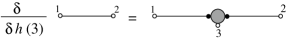
Figure 5: Graphical representation of Eq. (LABEL:DerivGh0) for the functional derivative of a $-\tilde{G}$ bond.

In appendix E, we use the graphical rules given in Figs. 3 and 5 to show that the functional derivative of any diagram $\Gamma$ of $L$ root vertices, $\tilde{\Omega}$ field vertices, and $-\tilde{G}$ bonds is given by the sum of all diagrams that may be obtained by adding one root circle to any vertex or by inserting a $\Omega^{(3)}$ vertex with one root circle into any bond of $\Gamma$. All of the diagrams that contribute to Eq. (89) for $S^{(n)}$ may be obtained, using this rule, by functional differentiation of $L_{\rm ref}$, $\ln\Xi_{\rm harm}$, or $\ln\Xi_{\rm anh}$: Differentiation of $L_{\rm ref}$ yields $\tilde{\Omega}^{(n)}$. Differentiation of $\ln\Xi_{\rm harm}$ is found to yield all of the one-loop diagrams described in Eq. (88). All of the remaining diagrams in Eq. (89) can be obtained by differentiation of one of the diagrams in the $-\tilde{G}$ bond expansion of $\ln\Xi_{\rm anh}$.

11 Intramolecular Correlations

A diagrammatic expression for the intramolecular cluster function $\Omega_{a}^{(n)}(1,\ldots,n)$ may be obtained by the following thought experiment: We mentally divide the $M_{a}$ molecules of species $a$ within a fluid of interest into two subspecies, such that a minority “labelled” subspecies has a number density $\epsilon\rho_{a}$ and majority “unlabelled” subspecies has a number density $(1-\epsilon)\rho_{a}$, with $\epsilon\ll 1$. In addition, we imagine dividing the monomers of each chemical type $i$ into labelled and unlabelled “types”, by making the monomers on the labelled subspecies of molecular species $a$ conceptually distinct from chemically identical monomers on any other species of molecule. This mental labelling of particular molecules and the monomers they contain is analogous to the procedure used to measure intramolecular correlations by neutron scattering, in which a small fraction of the molecules of a species are labelled by deuteration.

Consider the collective cluster function $S^{(n)}(1,\ldots,n)$ for a set of labelled monomers of types $\underline{i}=\{i_{,}\ldots,i_{n}\}$ that exist only on molecules belonging to the minority subspecies of species $a$. In the limit $\epsilon\rightarrow 0$, this function will be dominated by contributions that arise from correlations of monomers on the same labelled molecule of species $a$. The single-molecule intramolecular cluster function $\omega_{a}^{(n)}(1,\ldots,n)$ may thus be obtained from the limit

$$\omega_{a}^{(n)}(1,\ldots,n)=\lim_{\epsilon\rightarrow 0}\frac{1}{\epsilon\rho_{a}}S^{(n)}(1,\ldots,;\epsilon)$$ (91)

where $\epsilon\rho_{a}$ is the number density of the labelled subspecies of $a$ , and $S^{(n)}(1,\ldots,n;\epsilon)$ is the collective cluster function for the specified set of labelled monomer types as a function of $\epsilon$. The value of $\Omega_{a}(1,\ldots,n)$ for all of species $a$, without distinguishing labelled and unlabelled subspecies, may then be obtained by evaluating the product $\Omega_{a}\equiv\rho_{a}\omega_{a}$. Multiplication of Eq. (91) for $\omega_{a}$ by $\rho_{a}$ yields

$$\Omega_{a}^{(n)}(1,\ldots,n)=\lim_{\epsilon\rightarrow 0}\frac{1}{\epsilon}S^{(n)}(1,\ldots,n;\epsilon)$$ (92)

in which the l.h.s. is the desired value in the unlabelled fluid, with $\rho_{a}$ molecules of type $a$ per unit volume.

We may use Eq. (87) or (89) to expand the collective cluster function $S^{(n)}(1,\ldots,n;\epsilon)$ from the r.h.s. of Eq. (92) as an infinite set of diagrams. In what follows, we will refer to monomer types and vertex circles that are associated with the labelled subspecies of molecular species $a$ as labelled monomer types and circles, and vertices with labelled circles as labelled vertices. Because labelled molecules of type $a$ may contain only labelled monomer types, which cannot exist on any other species of molecule, the circles associated with each vertex must either be all labelled, or all unlabelled. Each labelled $\tilde{\Omega}$ vertex in a diagram is associated with a factor of $\epsilon\tilde{\rho}_{a}\tilde{\omega}_{a}$. Because each labelled vertex thus carries a prefactor of $\epsilon$, independent of the number of associated root circles, and because the diagram must contain a total of $n$ labelled root circles on one or more labelled root vertex, the dominant contribution to $S^{(n)}(1,\ldots,n;\epsilon)$ for a set of labelled monomer types in the limit $\epsilon\rightarrow 0$ is given by the set of diagrams in which the only labelled vertex in the diagram is a single root vertex that contains all $n$ root circles. Dividing the value of any such diagram by $\epsilon$, as required by Eq. (92), simply converts the factor of $\epsilon\tilde{\rho}_{a}\tilde{\omega}_{a}$ associated with its root vertex into a factor of $\tilde{\Omega}_{a}$. The desired expansion of the intramolecular correlation function $\Omega_{a}$ for any molecule of species $a$ in the unlabelled fluid is thus

L field vertices, −K bonds, anda single Ω~a root vertex withn root circles labelled 1,…,n}superscriptsubscriptΩ𝑎𝑛1…𝑛 fragmentsL field vertices, K bonds, andfragmentsa single ~Ω𝑎 root vertex withfragmentsn root circles labelled 1,…,n\Omega_{a}^{(n)}(1,\ldots,n)=\left\{\begin{tabular}[]{l}Sum of connected diagrams of\\ $L$ field vertices, $-K$ bonds, and\\ a single $\tilde{\Omega}_{a}$ root vertex with\\ $n$ root circles labelled $1,\ldots,n$\end{tabular}\right\}

$${\mathrm{\Omega }}_a^{(n)}(1,\mathrm{\dots },n)=\{\begin{array}{c}\end{array}$$Sum of connected diagrams ofSum of connected diagrams of (93)

Here, the bonds may be either $-U$ or $-\tilde{G}$ bonds, if the corresponding rules for the construction of valid diagrams are obeyed. Note that the set described on the r.h.s. includes the diagram containing one $\tilde{\Omega}_{a}$ root vertex and no bonds, shown as diagram (a) of Fig. (4). Diagrams (b)-(e) of Fig. (4) also contribute to expansion (93), if the root vertex in each diagram is interpreted as an $\tilde{\Omega}_{a}$ vertex.

In what follows, we will also need an expansion of the function $\Omega^{(n)}(1,\ldots,n)$ that is defined in Eq. (17) as a sum of single-species correlation functions. Diagrammatic expansions of $\Omega_{a}^{(n)}$ for different species $a$ but the same set $\underline{i}$ of monomer types contain topologically similar diagrams that differ only as a result of the different species labels associated with the $\tilde{\Omega}_{a}$ root vertex. The sum of a set of such otherwise identical diagrams, summed over all all values of species $a$, is equal to the value of a single diagram in which the root vertex is taken to be an $\tilde{\Omega}$ vertex, where $\tilde{\Omega}^{(n)}$ is defined by Eq. (37). Thus,

$$\begin{array}[]{rcl}\Omega^{(n)}(1,\ldots,n)=\left\{\begin{tabular}[]{l}Sum of connected diagrams of $L$\\ field vertices, $-K$ bonds, and a\\ single $\tilde{\Omega}$ root vertex with $n$\\ root circles labelled $1,\ldots,n$\end{tabular}\right\}\end{array}$$ (94)

The only difference between Eq. (94) and Eq. (93) is the nature of the function associated with the root vertex.

12 Molecular Number Density

A diagrammatic expansion for the average number density $\rho_{a}=\langle M_{a}\rangle/V$ for molecules of species $a$ may be obtained by applying the identity

$$\langle M_{a}\rangle=\left.\lambda_{a}\frac{\partial\ln\Xi}{\partial\lambda_{a}}\right|_{h}$$ (95)

to the diagrammatic expansion of $\ln\Xi$. Application of the operation $\lambda_{a}\frac{\partial}{\partial\lambda_{a}}$ to the function $\tilde{\Omega}$ vertex yields

$$\lambda_{a}\frac{\partial\tilde{\Omega}^{(n)}(1,\ldots,n)}{\partial\lambda_{a}} = \sum_{b}\tilde{\rho}_{a}\frac{\partial[\tilde{\rho}_{b}\tilde{\omega}_{b}^{(n)}(1,\ldots,n)]}{\partial\tilde{\rho}_{a}}$$ (96)

$$= \tilde{\Omega}_{a}^{(n)}(1,\ldots,n)\;\;.$$

Here, we have used the fact that the density $\tilde{\rho}_{a}$ in the ideal gas reference state, which is given by Eq. (35), is directly proportional to $\lambda_{a}$ at fixed $h$. The effect of the operation $\lambda_{a}\frac{\partial}{\partial\lambda_{a}}$ upon an $\tilde{\Omega}$ vertex is thus to transform it into a $\tilde{\Omega}_{a}$ root vertex.

By applying this operation to all of the vertices in a diagram, and repeating the reasoning used in Sec. 10 to generate equivalent sets of diagrams of $-U$ bonds and $-\tilde{G}$ bonds, we obtain a diagrammatic expansion

$$\rho_{a}=\tilde{\rho}_{a}+\frac{1}{V}\left\{\begin{tabular}[]{l}Sum of connected diagrams of\\ $L$ field vertices, one or more\\ $-K$ bonds, and a single $\tilde{\Omega}_{a}$\\ root vertex, with no root circles\end{tabular}\right\}$$ (97)

in which (again), $-K$ bonds may be either $-U$ or $-\tilde{G}$ bonds. Examples are given in Fig. 6.

Figure 6: Diagrams that contribute to expansion (97) for $\rho_{a}$, using diagrams of $-U$ bonds, $\tilde{\Omega}$ field vertices, and a single $\tilde{\Omega}_{a}$ root vertex with no root circles. Here, because there are no root circles to distinguish root and field vertices, the $\tilde{\Omega}_{a}$ root vertex is distinguished by being whitened.

13 Vertex Renormalization

We now discuss a topological reduction that allows infinite sums of diagrams of $\tilde{\Omega}$ vertices, in which the vertices represent ideal gas intramolecular correlation functions, to be reexpressed as corresponding diagrams of $\Omega$ vertices, in which the vertices represent the intramolecular correlation functions obtained in the interacting fluid of interest. The required procedure is closely analogous to one described briefly by Chandler and Pratt in their Mayer cluster expansion for flexible molecules [8]. It is analogous in a broader sense to the procedure used in the Mayer cluster expansion for simple atomic liquids to convert an activity expansion into a density expansion [3].

The following definitions will be needed in what follows:

A connecting vertex is one whose removal would divide the component that contains that vertex into two or more components. By the removal of a vertex, we mean a process in which the large circle and associated smaller circles representing the vertex and its arguments are all erased. Any bonds that were attached to the field circles of the removed vertex must instead be terminated at free root circles, whose spatial and monomer type arguments become parameters in mathematical expression represented by the diagram.

The components that are created by the removal of a connecting vertex are referred to as lobes of the corresponding component of the original diagram. A connecting circle thus always connects two or more lobes. A lobe is rooted if, before the removal of the connecting vertex, it contained at least one root circle (excluding those created by the removal of the vertex, which correspond to field circles of the removed vertex), and rootless otherwise.

An articulation vertex is a connecting vertex that is connected to at least one rootless lobe. A nodal vertex is a connecting vertex that connects at least two rooted lobes. It is possible for a connecting vertex that is connected to three or more lobes to be both a nodal vertex and an articulation vertex.

In the remainder of this section, we consider a topological reduction of expansions of various correlation functions and of the molecular density as sums of diagrams of $-U$ bonds and $\tilde{\Omega}$ vertices. The reduction discussed in this section is not directly applicable to diagrams of $-\tilde{G}$ bonds, for reasons that are discussed below.

13.1 Single-Molecule Properties

We first consider the reduction of expansion (94) for $\Omega^{(n)}$ as an infinite sum of diagrams of $-U$ bonds and $\tilde{\Omega}$ vertices. Let ${\bf A}$ be the infinite set of such diagrams described in Eq. (94). Let ${\bf B}$ be the subset of ${\bf A}$ that contain no articulation field vertices, which will be refer to as “base diagrams”. The desired reduction is based upon the observation that each of the diagrams in set ${\bf A}$ may be derived from a unique base diagram in subset ${\bf B}$ by “decorating” each field vertex with $n$ circles in the base diagram by one of the diagrams described in expansion (94) of $\Omega^{(n)}$. The “decoration” of a vertex is illustrated in Fig. (7): To decorate a vertex $v$ with $n$ circles with a pendant subdiagram $\gamma$ that contains a unique root vertex with $n$ root circles, we superpose the root vertex of subdiagram $\gamma$ onto vertex $v$ of the base diagram, superpose the root circles of $\gamma$ onto the circles of $v$, and blacken any circles that correspond to field circles of vertex $v$ in the base diagram.

Figure 7: An example of the “decoration” of a vertex by a pendant subdiagram: Diagram (c) is derived from diagram (a) by decorating the upper field vertex of (a) with subdiagram (b). In diagram (c), the $n=5$ field vertex to which diagram (b) has been attached is an articulation vertex.

This observation about the topology of diagrams is converted into a precise statement about their values by the vertex decoration theorem given in appendix F.3, which is a generalization of lemma 4 of Hansen and MacDonald. As a special case of this theorem, we find the following:

Theorem: Let $\Gamma$ be a diagram of $-U$ bonds and vertices, in which some specified set of “target” vertices are $\Omega$ vertices, none of which may be articulation vertices, each of which must contain exactly $n$ field and/or root circles. The value of $\Gamma$ is equal to the sum of the values of all diagrams that can be obtained by decorating each of these target vertices with any one of the diagrams belonging to the set described on the r.h.s. of Eq. (94) for $\Omega^{(n)}$.

To show the equivalence of the sum of a specified set ${\bf A}$ of diagrams of $\tilde{\Omega}$ vertices with the sum of a corresponding set ${\bf B}$ of base diagrams, we must show that every diagram in ${\bf A}$ can be obtained by decorating the target vertices of a unique base diagram in set ${\bf B}$, and, conversely, that every diagram that may be obtained by decorating the target vertices of a diagram in ${\bf B}$ is in ${\bf A}$. In cases of interest here, the base diagram of a diagram in set ${\bf A}$ may be identified by a graphical process in which we “clip” rootless lobes off of target vertices of derived diagrams until the diagram contains no more articulation target vertices.

Applying this reduction to all of the field vertices in all of the diagrams in expansion (94) for $\Omega^{(n)}$ yields the following renormalized expansion

$$\Omega^{(n)}(1,\ldots,n)=\left\{\begin{tabular}[]{l}Sum of connected diagrams\\ containing any number of $\Omega$ field\\ vertices and $-U$ bonds, and a\\ single $\tilde{\Omega}$ root vertex containing $n$\\ root circles labelled $1,\ldots,n$, with\\ no articulation field vertices\end{tabular}\right\}$$ (98)

This provides a recursive expressions for $\Omega^{(n)}$ vertices for all $n$. A corresponding expansion of $\Omega_{a}$ may be obtained by replacing the root $\tilde{\Omega}$ vertex by an $\tilde{\Omega}_{a}$ vertex with a specified species $a$.

In this reduction, we renormalize the field vertices, creating $\Omega$ field vertices, but leave the root vertex as an unrenormalized $\tilde{\Omega}$ vertex. As one way of seeing why the root vertex must be left unrenormalized, note that information about the intramolecular potential of an isolated molecule enters this set of relationships for $\Omega^{(n)}$ only through our use of an ideal gas correlation function for the root vertex: If we had managed to replace the factor of $\tilde{\Omega}$ associated with the root vertex by factor of $\Omega$, the resulting theory would not have contained any information about the intramolecular potential.

It may also be shown that the the single root vertex generally cannot be taken to be a target vertex of this topological reduction, because a diagram of $\tilde{\Omega}$ vertices and $-K$ bonds with a single root vertex that is an articulation vertex (i.e., is connected to two or more rootless lobes) generally cannot be related to a unique base diagram by the clipping process described above. To see this, imagine a process in which we first clip all rootless lobes off all of articulation field vertices in such a diagram, and then clip off all but one of the rootless lobes connected to the root diagram. The resulting diagram contains no articulation vertices, but is clearly not a unique base diagram, because the process requires an arbitrary choice of which of the lobes connected to the root vertex to leave “unclipped” in the final step.

Reasoning essentially identical to that applied above to $\Omega$ may also be applied to expansion (97) of $\rho_{a}$ about an ideal gas reference state as a sum of diagrams of $-U$ bonds. In this case, taking all of the field vertices to be target vertices yields

$$\rho_{a}=\tilde{\rho}_{a}+\frac{1}{V}\left\{\begin{tabular}[]{l}Sum of connected diagrams of $\Omega$\\ field vertices, one or more $-U$\\ bonds, and a single $\tilde{\Omega}_{a}$ root vertex\\ of species $a$ with no root circles,\\ with no field articulation vertices\end{tabular}\right\}\;\;.$$ (99)

13.2 Collective Cluster Functions

We next consider the topological reduction of expansion (87) for $S^{(n)}$. In this case, we consider the set ${\bf A}$ of diagrams described in Eq. (87). We divide this into a subset in which all $n$ root circles are on a single root vertex, which yields expansion (94) for $\Omega$, and a set ${\bf B}$ of all diagrams that contain two or more root vertices. Let ${\bf C}$ be the subset of diagrams in ${\bf B}$ that contain no articulation vertices, which we will refer to a base diagrams. The reader may confirm that any diagram in ${\bf B}$ (i.e., any diagram in ${\bf A}$ with two or more root vertices) may be derived from a unique base diagram in set ${\bf C}$ by decorating all of the vertices of the base diagram, including the root vertices, with one of the diagrams in the expansion of $\Omega$. The base diagram in set ${\bf C}$ corresponding to any diagram in set ${\bf B}$ may be unambiguously identified by the clipping process described above, which in this case yields a unique result in which none of the root or field vertices are connected to rootless lobes. Topologically reducing set ${\bf B}$ thus yields an expression for $S^{(n)}$ as

$$\begin{array}[]{rcl}S^{(n)}(1,\ldots,n)&=&\Omega^{(n)}(1,\ldots,n)\\ &+&\left\{\begin{tabular}[]{l}Sum of connected diagrams\\ of $\Omega$ vertices and $-U$ bonds\\ with $n$ roots circles labelled\\ $1,\ldots,n$ on two or more root\\ vertices, with no articulation\\ vertices\end{tabular}\right\}\end{array}$$ (100)

Here, the contribution $\Omega^{(n)}(1,\ldots,n)$, which may be represented as a diagram consisting one $\Omega^{(n)}$ vertex and no bonds, is obtained by summing the subset of diagrams in ${\bf A}$ in which all of the root circles are on one vertex.

The topological reduction discussed in this section provides a rigorous basis for the separation of the calculation of collective correlation functions into:

1. A calculation of collective correlation functions, via Eq. (100), as functionals of the actual intramolecular correlation functions in the fluid of interest, and

2. A calculation of the effect of non-covalent interactions upon the intramolecular correlation functions, via Eq. (98).

In fluids of point particles or rigid molecules, in which the intramolecular correlations are either trivial or known a priori, the analogous topological reduction allows an activity expansion to be converted into a density expansion. In fluids of flexible molecules, this conversion is incomplete. In expansion (100) of the collective cluster functions, the intramolecular correlation functions $\Omega^{(n)}$ play a role partially analogous to that of the number density in the corresponding expansion for an atomic liquid. Because expansion (98) of $\Omega^{(n)}_{a}$ still contains an explicit factor of the molecular activity $\lambda_{a}$ associated with the root vertex, however, the reduction does not allow either intramolecular or collective correlation functions to be expanded as explicit functions of molecular density. Explicit expansions of $\Omega_{a}^{(n)}$, $\omega_{a}^{(n)}$, $\mu_{a}$, and the Helmholtz free energy as functions of molecular number density will be derived in a subsequent paper.

The topological reduction discussed above cannot be directly applied to diagrams of $\tilde{\Omega}$ vertices and $-\tilde{G}$ bonds, in which the bonds represent screened interactions. Such diagrams may contain articulation field vertices for which all but two circles are attached by $-\tilde{G}$ bonds to rootless lobes. Clipping all of the rootless lobes from such a vertex and re-interpreting the bonds as $G$ bonds would yield a field vertex with two circles, creating an invalid base diagram of $-G$ bonds. To obtain expansions of the quantities of interest in terms of diagrams of $\Omega$ vertices with bonds that represent a screened interaction, it necessary to first complete the above renormalize of the vertices in an expansion with $-U$ bonds, and then resum chains of $-U$ bonds to obtain a modified screened interaction, in which $\tilde{\Omega}$ is replaced by $\Omega$ in the definition. This further renormalization of the bonds is discussed in Sec. 15.

14 Leaf Subdiagrams and Shifts of Reference Field

The renormalization of vertices discussed above was applied to an expansion about an ideal gas reference state, with $J^{*}=0$, in terms of diagrams with $-U$ bonds and $\tilde{\Omega}$ vertices. In each of the diagrams described in expansion (98) of $\Omega^{(n)}_{a}$ or in expansion (99) of $\rho_{a}$, the factor of $\tilde{\Omega}_{a}$ associated with the root vertex must thus be evaluated using the molecular number density $\tilde{\rho}_{a}[h]$ obtained for a non-interacting gas in a field $\tilde{h}=h$, rather than the molecular number density obtained from the Flory-Huggins equation of state.

In both expansions (98) and (99), the root vertex of each diagram may be an articulation vertex. Among the types of rootless lobes that may be attached to the root vertices in these diagrams is a simple “leaf” subdiagram, that consists of a single $-U$ bond attached at one end to the root vertex and at the other to a $\Omega^{(1)}$ field vertex, as shown in Fig. (8). The terminal $\Omega^{(1)}$ vertex represents a factor of monomer concentration, since $\Omega^{(1)}_{i}({\bf r})\equiv\langle c_{i}({\bf r})\rangle$. In this section, we consider a partial renormalization of the root vertex in each of the diagrams of expansion (98) or expansion (99), in which we show that the contributions of such leaf subdiagrams may be absorbed into a shift of the value of the field $\tilde{h}$ used to evaluate the factor of $\tilde{\Omega}$ associated with the root vertex.

The value of a single leaf subdiagram, viewed as a coordinate space diagram with generic field circle and one free root circle, is given by the convolution

$$\phi_{i}({\bf r})\equiv\sum_{j}\int\!d{\bf r}^{\prime}\;U_{ij}({\bf r}-{\bf r}^{\prime})\langle c_{j}({\bf r}^{\prime})\rangle$$ (101)

The field $\phi$ is quite literally a mean field, since it is equal to the ensemble average of the potential $\int d(2)\;U(1,2)*c(2)$ produced by a fluctuating monomer density field. Note that the average monomer concentration $\langle c_{j}({\bf r}^{\prime})\rangle$ in this equation is the actual value in the interacting fluid, because the corresponding $\Omega^{(1)}(2)=\langle c(2)\rangle$ vertex has already been renormalized by the reduction discussed in the previous section.

Let $\Gamma^{(n,m)}(1,\ldots,n)$ be a diagram with generic field circles that consists of a single $\tilde{\Omega}^{(n+m)}$ vertex with $n$ root circles, with arguments $1,\ldots,n$, and $m$ field circles, to which are attached $m$ pendant leaf subdiagrams, like those shown in Fig. (8). The value of such a diagram is given, in compact notation, by an integral

$$\Gamma^{(n,m)} = \frac{1}{m!}\int d(n+1)\cdots\int d(n+m)$$

$$\times\tilde{\Omega}^{(n+m)}(1,\ldots,n+m)\phi(n+1)\cdots\phi(n+m)$$

where $m!$ is a symmetry number equal to the number of possible permutations of the indistinguishable pendant leaves. Let the sum of all such diagrams, with any number of leaves, define a function

$$\bar{\Omega}^{(n)}_{a}(1,\ldots,n)\equiv\sum_{m=0}^{\infty}\Gamma^{(n,m)}$$ (103)

The function $\tilde{\Omega}^{(n+m)}(1,\ldots,n)$ in Eq. (14), which is evaluated in an ideal gas subjected to a field $\tilde{h}=h$, is an $m$-th functional derivative of $\tilde{\Omega}^{(n)}(1,\ldots,n;\tilde{h})$ with respect to the applied field $\tilde{h}$, at fixed molecular activity. The sum obtained by substituting Eq. (14) into Eq. (103) is a functional Taylor series expansion about $\tilde{h}=h$ of a quantity

$$\bar{\Omega}^{(n)}_{a}(1,\ldots,n)\equiv\tilde{\Omega}^{(n)}_{a}(1,\ldots,n;[\bar{h}])$$ (104)

in which $\tilde{\Omega}^{(n)}(1,\ldots,n;[\bar{h}])$ is an intramolecular correlation function in an ideal gas that is subjected to a field

$$\bar{h}(1)\equiv h(1)+\phi(1)\quad.$$ (105)

The field $\bar{h}$ is closely related, but not identical, to the saddle-point field $\tilde{h}^{s}$ used in the mean field approximation. The difference arises from the fact that the grand-canonical mean field theory uses a self-consistently determined estimate of $\langle c(1)\rangle$ for a system with a specified set of chemical potentials, whereas $\bar{h}(1)$ is calculated here using the exact average value $\langle c(1)\rangle$ to calculate $\phi$.

Figure 8: Diagrams consisting of one root $\tilde{\Omega}_{a}^{(n)}$ vertex attached to $m$ leaf subdiagrams, which are denoted $\Gamma^{(n,m)}$ in the text, for $n=3$ and $m=1,\ldots,4$. The sum over all $m$, for fixed $n$, yields the correlation function $\bar{\Omega}^{(n)}_{a}$ for a molecule with a specified activity $\lambda_{a}$ in a mean field $\phi(1)\equiv\int d(2)U(1,2)\langle c(2)\rangle$

In what follows, we will use the corresponding notation

$$\bar{\rho}_{a}\equiv\tilde{\rho}_{a}(\lambda;[\bar{h}])$$ (106)

to denote the value of average molecular number density of species $a$ obtained in grand-canonical ensemble for an ideal gas subsected to a mean field $\bar{h}$. Because of the lack of self-consistency in the definition of $\bar{h}$, the values of $\bar{\rho}_{a}$, which are an approximation for the true molecular number densities, are generally not consistent with the exact values of $\langle c(1)\rangle$ used to calculate $\bar{h}$. In a homogeneous fluid, the only effect of a shift of the reference field $\tilde{h}$ used to calculate $\tilde{\Omega}^{(n)}_{a}$ is to change value of the corresponding molecular density $\tilde{\rho}_{a}(\lambda,h)$ to $\bar{\rho}_{a}$, without modifying $\tilde{\omega}^{(n)}_{a}$.

It follows from a straightforward application of the vertex decoration theorem of appendix subsection F.3, and from our identification of $\bar{\Omega}$ as the sum of subdiagrams consisting of a root $\tilde{\Omega}$ vertex with any number of pendant leaves, that

$$\Omega^{(n)}_{a}(1,\ldots,n)=\left\{\begin{tabular}[]{l}Sum of connected diagrams\\ containing any number of $\Omega$ field\\ vertices and $-U$ bonds, and a\\ single $\bar{\Omega}_{a}$ root vertex containing\\ $n$ root circles labelled $1,\ldots,n$,\\ with no articulation field\\ vertices, and no $\Omega^{(1)}$ vertices\end{tabular}\right\}$$ (107)

Note that the prohibition on $\Omega^{(1)}$ field vertices in Eq. (107) is equivalent to a prohibition on diagrams with leaf subdiagrams. Applying essentially identical reasoning to expansion (99) of $\rho_{a}$ yields the expansion

$$\rho_{a}=\bar{\rho}_{a}+\frac{1}{V}\left\{\begin{tabular}[]{l}Sum of connected diagrams\\ containing any number of $\Omega$ field\\ vertices, one or more $-U$ bonds,\\ and a single $\bar{\Omega}_{a}$ root vertex with\\ no root circles, no articulation field\\ vertices, and no $\Omega^{(1)}$ vertices\end{tabular}\right\}$$ (108)

In a homogeneous liquid, the $\bar{\Omega}_{a}$ root vertex in Eq. (107) may be replaced by a product $\bar{\rho}_{a}\tilde{\omega}_{a}$, thus absorbing the effect of the mean field $\phi$ into an overall prefactor of $\bar{\rho}_{a}$.

15 Screened Interaction

In this section, we obtain an expansion in terms of renormalized vertices with bonds that represent a redefined screened interaction. Starting from expansion (98) or (100) of a correlation or cluster function in diagrams with $-U$ bonds and $\Omega$ field vertices, we may obtain an effective screened interaction by summing chains of alternating $\Omega^{(2)}$ vertices and $-U$ bonds. Repeating the reasoning outlined in Sec. 9, we find that the resummation of all possible chains of alternating $-U$ bonds and $\Omega^{(2)}$ field vertices yields an effective screened interaction $G(1,2)$, where

$$G^{-1}(1,2)\equiv\Omega(1,2)+U^{-1}(1,2)$$ (109)

The function $G$ is exactly analogous to $\tilde{G}$, except for the replacement of the ideal gas correlation function $\tilde{\Omega}^{(2)}(1,2)$ by the corresponding function $\Omega(1,2)\equiv\Omega^{(2)}(1,2)$ for a molecule in the interacting liquid.

Resumming chain subdiagrams of $-U$ bonds and $\Omega^{(2)}$ field vertices in Eqs. (107) and (108) yields the alternate expansions

$$\Omega_{a}^{(n)}(1,\ldots,n)=\left\{\begin{tabular}[]{l}Sum of connected diagrams of\\ $-G$ bonds, $\Omega$ field vertices, and\\ a single $\bar{\Omega}_{a}$ root vertex with $n$\\ root circles with arguments\\ $1,\ldots,n$, no articulation field\\ vertices, and no $\Omega^{(1)}$ or $\Omega^{(2)}$\\ field vertices\end{tabular}\right\}$$ (110)

and

$$\rho_{a}=\bar{\rho}_{a}+\frac{1}{V}\left\{\begin{tabular}[]{l}Sum of connected diagrams of $-G$\\ bonds, $\Omega$ field vertices, and a single\\ $\bar{\Omega}_{a}$ root vertex with no root circles,\\ with no articulation field vertices,\\ and no $\Omega^{(1)}$ or $\Omega^{(2)}$ field vertices\end{tabular}\right\}$$ (111)

Applying the same reduction to Eq. (100) for the collective cluster functions yields

$$\begin{array}[]{rcl}S^{(n)}(1,\ldots,n)&=&\Omega^{(n)}(1,\ldots,n)\\ &+&\left\{\begin{tabular}[]{l}Sum of connected diagrams of $\Omega$\\ vertices and one or more $-G$ bonds,\\ with $n$ root circles labelled $1,\ldots,n$\\ on two or more root vertices, no\\ articulation vertices and no $\Omega^{(2)}$\\ field vertices\end{tabular}\right\}\end{array}$$ (112)

In Eq. (112), no explicit prohibition on $\Omega^{(1)}$ vertices is required, because they are already excluded by the prohibition on articulation vertices.

Figure 9: Diagrams of $G$ bonds, $\Omega$ field vertices, and a $\bar{\Omega}_{a}$ root vertex that that contribute to expansion (110) of $\Omega_{a}^{(2)}$.

Expansions (110-112) are essentially vertex-renormalized versions of the expansions of the corresponding quantities about a Flory-Huggins reference field in terms of diagrams of $\tilde{G}$ bonds and $\tilde{\Omega}$ vertices. Both types of expansion prohibit diagrams with 1- and 2-point field vertices, and thus yield diagrams with similar topology, in which the vertices and bonds have similar meanings. They differ only as a result of the replacement in the renormalized expansions of $\tilde{\Omega}$ field vertices by $\Omega$ vertices, and of $\tilde{G}$ bonds by $G$ bonds, and the corresponding prohibition in the renormalized expansions on diagrams with articulation field vertices.

16 Bond-Irreducible Diagrams

The diagrammatic expansion of the two-point cluster function $S(1,2)$ may be simplified by relating $S$ to a quantity $\Lambda(1,2)$ that we define as the sum of all bond-irreducible two-point diagrams. A diagram is said here to be bond-irreducible if it is connected and cannot be divided into two or more components by removal of any single bond. By the removal of a bond, we mean the erasure of the bond, the erasure of any free root circles to which it is attached, and the transformation of any vertex field circles to which it is attached into vertex root circles.

We define

$$\Lambda(1,2)=\left\{\begin{tabular}[]{l}Sum of bond irreducible diagrams\\ of 1 or 2 $\tilde{\Omega}$ root vertices and any\\ number of $L$ field vertices and $-K$\\ bonds, with 2 root circles labelled\\ $1$ and $2$\\ \end{tabular}\right\}$$ (113)

The set of diagrams described in on the r.h.s. of Eq. (113) also includes a subset of diagrams in which both root circles are on a single vertex. Among these is the trivial diagram consisting of a single $\tilde{\Omega}^{(2)}$ vertex and no bonds. The sum of this infinite subset of diagrams yields the diagrammatic expansion of $\Omega^{(2)}(1,2)$. We may thus distinguish inter- and intra-molecular contributions to $\Lambda(1,2)$ by writing

$$\Lambda(1,2)=\Omega^{(2)}(1,2)+\Sigma(1,2)$$ (114)

where

with two Ω~ root vertices, any numberof L field vertices and −K bonds,with 2 vertex root circles labelled 1and 2 on different root vertices}Σ12 fragmentswith two ~Ω root vertices, any numberfragmentsof L field vertices and K bonds,fragmentswith 2 vertex root circles labelled 1fragmentsand 2 on different root vertices\Sigma(1,2)\equiv\left\{\begin{tabular}[]{l}Sum of bond irreducible diagrams\\ with two $\tilde{\Omega}$ root vertices, any number\\ of $L$ field vertices and $-K$ bonds,\\ with 2 vertex root circles labelled $1$\\ and $2$ on different root vertices\end{tabular}\right\}

$$\mathrm{\Sigma }(1,2)\equiv \{\begin{array}{c}\end{array}$$Sum of bond irreducible diagramsSum of bond irreducible diagrams (115)

Renormalizing both vertices and bonds yields the equivalent expansion

$$\Sigma(1,2)=\left\{\begin{tabular}[]{l}Sum of bond-irreducible diagrams\\ of $\Omega$ vertices and $-G$ bonds, with\\ $2$ root circles labelled $1$ and $2$ on\\ different vertices, with no\\ articulation vertices\end{tabular}\right\}$$ (116)

in which field vertices with two circles are prohibited.

Figure 10: Examples of diagrams of $G$ bonds and $\Omega$ field vertices that contribute to expansion (116) of $\Sigma(1,2)$.

The expansion of $S(1,2)$ in terms of $\tilde{\Omega}$ vertices and $-U$ bonds may be expressed diagrammatically as an infinite set of chains of alternating $-U$ bonds and $\Lambda$ field vertices, terminated at both ends by $\Lambda$ root vertices. This may be expressed algebraically as an infinite series

$$S = \Lambda-\Lambda*U*\Lambda+\cdots$$ (117)

$$= \Lambda-\Lambda*U*S\;\;.$$

Summing the series, or solving the recursion relation, yields an expression for the inverse structure function as

$$S^{-1}(1,2)=\Lambda^{-1}(1,2)+U(1,2)$$ (118)

Eq. (118) is an generalization of the random phase approximation for $S^{-1}$ in which $\Omega$ is replaced by $\Lambda$. The generalized Ornstein-Zernick relation of Eq. (20) is a different generalization in which $U$ is instead replaced by $-C$.

17 Direct Correlation Function

We now construct a diagrammatic expansion of the Ornstein-Zernicke direct correlation function $C$ defined in Eq. (20). This quantity may be related to the function $\Lambda$ by equating the r.h.s.’s of Eqs. (118) and (20) for $S^{-1}(1,2)$. This yields

$$C(1,2)\equiv-U(1,2)+\Delta C(1,2)$$ (119)

where

$$\Delta C(1,2)=-\Lambda^{-1}(1,2)+\Omega^{-1}(1,2)\;\;,$$ (120)

and where $\Lambda(1,2)=\Omega(1,2)+\Sigma(1,2)$.

By expanding $\Lambda^{-1}=[\Omega+\Sigma]^{-1}$ as a geometrical series, $\Delta C(1,2)$ may also be expressed as a convolution

$$\Delta C=\Omega^{-1}*T*\Omega^{-1}$$ (121)

in which

$$T \equiv \Sigma-\Sigma*\Omega^{-1}*\Sigma+\cdots$$ (122)

$$= \Sigma-\Sigma*\Omega^{-1}*T\;\;.$$

Summing this series, or solving the recursion relation, yields

$$T^{-1}(1,2)=\Sigma^{-1}(1,2)+\Omega^{-1}(1,2)$$ (123)

Eq. (122) provides a useful starting point for the construction of an explicit diagrammatic expansion of $T$.

17.1 Diagrammatic Expansions

To express Eq. (122) as a sum of diagrams, we depict each factor of $-\Omega^{-1}$ in the infinite series as a $-\Omega^{-1}$ bond, which will be represented by a dotted line. This yields an expansion of $T$ as

$$\begin{array}[]{rcl}T(1,2)&=&\left\{\begin{tabular}[]{l}Sum of diagrams containing any\\ number of $\Omega$ vertices, $-G$ bonds\\ bonds, and $-\Omega^{-1}$ bonds, with two\\ root circles with arguments $1$ and\\ and $2$ on different vertices, with\\ no articulation vertices, such that\\ the diagram cannot be divided into\\ components by cutting any one $-G$\\ bond, but can be so divided by\\ cutting any one $-\Omega^{-1}$ bond\end{tabular}\right\}\end{array}$$ (124)

As with any expansion in terms of $-G$ bonds, field vertices with exactly two circles are implicitly prohibited. The above description applies equally well to an expansion of $T(1,2)$ in terms of diagrams of $-U$ bonds, rather than $-G$ bonds, if $\Omega^{(2)}$ field vertices are allowed. Corresponding expansions of Eq. (121) for $\Delta C(1,2)$ may then be obtained by adding two external $-\Omega^{-1}$ bonds to each diagram in the expansion of $T$, as shown in Fig. (11).

An alternative expansion of $T$ may be obtained by viewing each diagram in expansion (124) as a necklace of “pearls”, where a pearl is a bond-irreducible subdiagram of $-G$ or $-U$ bonds and $\Omega$ vertices that contains no nodal vertices. The pearls of a diagram in expansion (124) are thus the disjoint components that would created by removing all $-\Omega^{-1}$ bonds and all nodal vertices. For example, in Fig. (11), diagrams (b) and (c) each contain two identical pearls, which are connected by a nodal vertex in diagram (b) and by an $-\Omega^{-1}$ bond in diagram (c). Diagram (d) contains 4 pearls.

Figure 11: Examples of diagrams that contribute to the expansion (124) for $T(1,2)$. Here, vertices are $\Omega$ vertices, solid lines are $-G$ bonds, and dashed lines are $-\Omega^{-1}$ bonds. A corresponding expansion of $\Delta C(1,2)$ may be obtained by attaching external $-\Omega^{-1}$ bonds to both root sites of each diagram in this expansion.

Each diagram in Eq. (124) for $T(1,2)$ may thus be viewed as a string of pearls, in which each pair of neighboring pearls may be connected by either a nodal vertex or by an $-\Omega^{-1}$ bond connecting two $\Omega$ vertices. The set of all such diagrams can be generated from the set of bond-irreducible two-point diagrams that contributes to Eq. (116) for $\Sigma$ by replacing every nodal vertex in any diagram in expansion (116) by either the original $\Omega$ vertex or by a subdiagram consisting of two vertices connected by a $-\Omega$ bond. Let

$$N^{(n,n^{\prime})}\equiv\Omega^{(n+n^{\prime})}+\Pi^{(n,n^{\prime})}$$ (125)

denote the sum of the two such subdiagrams shown, for $n=n^{\prime}=3$, in Fig. (12). Here, $\Pi^{(n,n^{\prime})}$ denotes the value of a subdiagram consisting of an $\Omega^{(n+1)}$ vertex and an $\Omega^{(n^{\prime}+1)}$ vertex connected by a $-\Omega^{-1}$ bond, in which one $\Omega^{(n+1)}$ vertex contains $n$ root circles labelled $1,\ldots,n$ and the $\Omega^{(n^{\prime}+1)}$ contains $n^{\prime}$ root circles labelled $1^{\prime},\ldots,n^{\prime}$, as shown for $n=n^{\prime}=3$ in the second diagram of Fig. (12). Let a nodal $N$ vertex be one in which the function $N^{(n,n^{\prime})}(1,\ldots,n;1^{\prime},\ldots,n^{\prime})$ is associated with an $(n+n^{\prime})$-point nodal vertex that is connected to one pearl by bonds connected to $n$ field circles $1,\ldots,n$ and to a second through $n^{\prime}$ field circles labelled $1^{\prime},\ldots,n^{\prime}$. An alternate expansion of $T$ may be obtained by replacing all of the nodal $\Omega$ vertices in expansion (116) of $\Sigma$ by nodal $N$ vertices. The corresponding expansion of $\Delta C$ is obtained by adding two external $-\Omega^{-1}$ bonds to each diagram in the expansion. For example, replacing the nodal $\Omega$ vertex in diagram (b) of (10) with an $N$ nodal vertex and then adding two external $-\Omega^{-1}$ bonds yields a diagram whose value is equal to the sum of the values of diagrams (b) and (c) in Fig. (11). Geometrical series (122) for $T(1,2)$ may thus be expressed as a sum

$$T(1,2)=\left\{\begin{tabular}[]{l}Sum of bond-irreducible diagrams of\\ vertices and $-G$ bonds, with two root\\ circles labelled $1$ and $2$ on different\\ $\Omega$ vertices, in which all nodal vertices\\ are $N$ vertices and all other vertices\\ are $\Omega$ vertices, with no articulation\\ vertices\end{tabular}\right\}$$ (126)

The above description applies equally well to a corresponding expansion of $T$ in terms of diagrams of $-U$ bonds, aside from the removal of the implicit prohibition on $\Omega^{(2)}$ field vertices.

17.2 Atomic Limit

Expansion (126) may be used to recover a simpler expression for $C$ in the limit of a liquid of point particles. For this purpose, it is convenient to consider the expansion of $T$ in terms of $-U$ bonds, rather than $-G$ bonds. In a homogeneous mixture of point particles, the normalized Fourier tranform $\Omega^{(n)}_{\underline{i}}(\underline{\bf k})$ is nonzero only when $i_{1}=i_{2}=\ldots=i_{n}=i$ and ${\bf k}_{1}+\cdots+{\bf k}_{n}=0$, and in this case is equal to the density $\rho_{i}$ of particles of type $i$. Using these relations, it is straightforward to show that the function $N^{(n,n^{\prime})}$ defined in Eq. (125) vanishes identically in the atomic limit.

Figure 12: Graphical representation of the quantity $N$ defined in Eq. (125). The quantity shown is $N^{(3,3)}(1,2,3,1^{\prime},2^{\prime},3^{\prime})$, where vertices are $\Omega^{(n)}$ vertices, and the dashed line represents a $-\Omega^{-1}$ bond. The second diagram is $\Pi^{(3,3)}$

Because the function $N$ that we associate with nodal vertices in (126) for $T$ vanishes, this expansion (126) for $T$ thus reduces in the atomic limit to a sum of bond-irreducible diagrams of $-\rho$ vertices and either $-G$ or $-U$ bonds with two root circles on different root circles, with no articulation vertices or nodal vertices. Such diagrams can thus have no connecting vertices. Adding two external legs with values $\Omega^{-1}_{ij}({\bf k})=\delta_{ij}\rho_{i}^{-1}$ to each diagram in the expansion of $T$ yields a corresponding expansion for $\Delta C$. The factors of $\rho_{i}^{-1}$ associated with these external legs cancel the factors of $\rho_{i}$ associated with the root vertices, thus converting the root vertices into “$1$ vertices” that introduce a factor of unity into the integrand of the corresponding integral. Such root $1$ vertices are represented as white circles in the conventional representation of cluster diagrams for atomic liquids. [3] By considering the resulting expansion of $\Delta C$ in the atomic limit in terms of diagrams of $-U$ bonds, and adding to this the diagram consisting of a single $-U$ bond to obtain $C=-U+\Delta C$, we obtain an expansion

$$C(1,2)=\left\{\begin{tabular}[]{l}Sum of diagrams of one or more $-U$\\ bonds, any number of field $\rho$ vertices,\\ and two root $1$ vertices labelled $1$\\ and $2$, with no connecting vertices\end{tabular}\right\}$$ (127)

for liquids of point particles. Note that the set described on the r.h.s. includes the diagram consisting of a single $-U$ bond, since this description does require that the diagrams be bond-irreducible, but the prohibition on connecting vertices automatically excludes all bond-reducible diagrams other than this trivial one. Eq. (127) is a perturbative cluster diagram variant of a well known expansion for $C(1,2)$ as a sum of Mayer cluster diagrams, given in Eq. (5.2.16) of Hansen and MacDonald [3]), in which the Mayer diagrams are required to satisfy the same topological constraints as those specified for perturbative cluster diagrams in Eq. (127).

18 Long Range Interactions and the Loop Expansion

The field-theoretic approach followed here leads naturally to a loop expansion about a mean field saddle point. The resulting expansion is useful, however, only if fluctuations about the mean field solution are small. In fluids of point particles, the mean field theory of Sec. 4 is known [41, 42, 43] to be exact in the so-called Kac limit of long-range interactions and/or high particle densities, in which each particle interacts weakly with many other particles.

To define this limit, we consider a class of models in which the pair interaction between monomers or (in an atomic liquid) atoms is of the form

$$U_{ij}({\bf r}-{\bf r}^{\prime})=\bar{U}_{ij}\gamma^{3}F(\gamma|{\bf r}-{\bf r}^{\prime}|)\;\;,$$ (128)

Here, $\bar{U}_{ij}$ is an interaction strength with units of volume, $\gamma^{-1}$ is an adjustable range of interaction, and $F({\bf x})=F(|{\bf x}|)$ is a dimensionless function that is required to satisfy a normalization condition $\int d{\bf x}\;F({\bf x})=1$. This parameterization yields a Fourier transform

$$U_{ij}({\bf k})=\bar{U}_{ij}\hat{F}({\bf k}/\gamma)\;\;,$$ (129)

in which $\hat{F}({\bf k})\equiv\int d{\bf x}\;e^{i{\bf k}\cdot{\bf x}}F({\bf x})$ is the Fourier transform of $F({\bf x})$, and in which $\hat{F}(0)=1$ as a result of the normalization assumed for $F({\bf x})$. To further simplify the argument, we will assume in what follows that $F({\bf x})$ is a function that falls off smoothly and rapidly with dimensionless separation $|{\bf x}|$, such as a Gaussian, and that, correspondingly, $\hat{F}({\bf q})$ decreases rapidly to zero for $|{\bf q}|\gg 1$.

The mean field theory for simple atomic fluids with interactions is known [41, 42, 43] to be asymptotically exact in the limit $\gamma\rightarrow 0$ of an infinitely long range, infinitely weak potential. In this limit, the first correction to mean field theory in an expansion in powers of $\gamma$ is given by the Gaussian approximation discussed in Sec. 5. We show below that this $\gamma$-expansion corresponds to a loop expansion of the perturbative cluster expansion. Interestingly, the loop expansion may be shown to remain valid even for nearly incompressible fluids with very strong repulsive interactions, if the pair potential is of sufficiently long range.

18.1 Nearly Incompressible Atomic Mixtures

As a simple example that retains some of the physics relevant to a dense molecular liquid, we first consider a simple model of a nearly incompressible binary mixture of point particles. We consider a mixture with a total particle number density $c\equiv c_{1}+c_{2}$, with interactions of the form given in Eqs. (128) and (129). The interaction matrix $\bar{U}_{ij}$ is taken to be of the form

$$\bar{U}_{ij}=\left[\begin{array}[]{cc}\bar{B}_{0}&\bar{B}_{0}+\bar{\chi}_{0}\\ \bar{B}_{0}+\bar{\chi}_{0}&\bar{B}_{0}\end{array}\right]\;\;\;,$$ (130)

This yields an interaction that reduces in the limit of slow spatial variations $q\ll\gamma$ to a continuum approximation

$$U_{int}\simeq T\int\!d{\bf r}\;\left\{\frac{1}{2}\bar{B}_{0}(c_{1}+c_{2})^{2}+\bar{\chi}_{0}c_{1}c_{2}\right\}\;\;.$$ (131)

In this form, it is clear that $\bar{B}_{0}$ is proportional to a mean-field compression modulus and that $\bar{\chi}_{0}$ is a measure of the mean field enthalpy of mixing. The quantities $\bar{B}_{0}$ and $\bar{\chi}_{0}$ have units of volume, and may be used to define dimensionless quantities $B_{0}\equiv\bar{B}_{0}c$ and $\chi_{0}\equiv\bar{\chi}_{0}c$. The quantity $\chi_{0}$ is a “bare” dimensionless Flory-Huggins parameter.

Consider the screened interaction $G$ for this model in the limit $B_{0}\gg 1$ of a nearly incompressible liquid. In the limit $k\ll\gamma$, for which $F({\bf k}/\gamma)\simeq 1$, taking the limit $B_{0}\rightarrow\infty$ of an infinitely strong bare repulsion yields a screened interaction

$${\bf G}({\bf k})\simeq\frac{1}{c-2\bar{\chi}_{0}c_{1}c_{2}}\left[\begin{array}[]{cc}1-2\bar{\chi}_{0}c_{2}&1\\ 1&1-2\bar{\chi}_{0}c_{1}\end{array}\right]\;$$ (132)

For any large but finite $B_{0}$, however, we will assume that a rapid decrease in $\hat{F}({\bf k}/\gamma)$ for ${\bf k}\gg\gamma$ causes both the bare interaction $U$ and the corresponding screened interaction $G$ to become negligible for $|{\bf k}|\gg\gamma$. In what follows, to characterize the relative magnitude of different contributions to the free energy at the level of power counting, this behavior will approximated by a sharp cutoff in which ${\bf G}({\bf k})$ is given by Eq. (132) for all $k<\gamma$, and ${\bf G}({\bf k})=0$ for $k>\gamma$. In an interaction site model, the inverse range of interaction $\gamma$ thus acts as a cutoff wavenumber for the screened interaction.

The Gaussian contribution to the Helmholtz free energy in the limit $B\gg 1$ is given in this approximation by an integral

$$\frac{\delta A}{V}=\frac{1}{2}\int\limits_{|{\bf k}|<\gamma}\ln[(c-2\bar{\chi}_{0}c_{1}c_{2})\bar{B}_{0}]\;\;.$$ (133)

This yields a contribution to the total free energy per particle of order $(\gamma^{3}/c)\ln(B)$, and a contribution to the free energy of mixing of order $\bar{\chi}_{0}\gamma^{3}$ per particle. For stable liquids, with $\chi_{0}\lesssim 1$, the Gaussian contribution to the free energy of mixing is thus small compared to the mean field contribution whenever $\gamma^{3}\ll c$.

18.2 Loop Expansion

We now consider the loop expansion of $\ln\Xi$ and its functional derivatives for this model. Consider the contribution of an arbitrary connected diagram $\Gamma$ of $-G$ bonds and $\tilde{c}$ vertices to an expansion of $\ln\Xi$ about the mean field reference state. We consider the Fourier space interpretation of $\Gamma/V$, which represents a contribution to the pressure $P=\ln\Xi/V$. Let the diagram of interest contain $n_{B}$ $\tilde{G}$ bonds and $n_{V}$ vertices. In a homogeneous fluid of point particles, each vertex simply represents a factor of $\tilde{c}$, independent of the number of field and/or root circles attached to the vertex. The number $n_{L}$ of independent wavevector integrals in the Fourier representation of the diagram in a homogeneous liquid, or the number of loops, is [23, 44]

$$n_{L}=n_{B}-n_{V}+1$$ (134)

To characterize the dependence of the value of the diagram upon $\gamma$ and $\tilde{c}$, at the level of power counting, we consider an approximation with sharp wavevector cutoff, in which we use Eq. (132) for $-\tilde{G}({\bf k})$ for bonds with $|{\bf k}|<\gamma$, and set $\tilde{G}=0$ for all $|{\bf k}|>\gamma$. In this approximation, in a system of point particles, the only length scale in the integrand is cutoff length $\gamma^{-1}$, and so it is convenient to non-dimensionalize all wavevectors by $\gamma$. After non-dimensionalization, the value $\Gamma/V$ will contain a prefactor of order $c$ from each vertex, a prefactor of $1/c$ from each $-G$ bond, and a prefactor of $\gamma^{3}$ from the measure of each independent wavevector integral (or loop), which multiply a non-dimensionalized Fourier integral. Using Eq. (134), we find an overall prefactor of order

$$\gamma^{3}(\gamma^{3}/c)^{n_{L}-1}$$ (135)

for any diagram with $n_{L}$ loops, where $c$ is an average particle concentration. Here, for the purposes of power counting, we have neglected the distinction between $c$ and the Flory-Huggins result for $\tilde{c}$. This prefactor multiplies a dimensionless Fourier integral in which the dimensionless wavevector ${\bf k}/\gamma$ associated with each bond of wavevector ${\bf k}$ is restricted to values $|{\bf k}|/\gamma<1$, and in which the integrand is a product of factors of $G_{ij}({\bf k})/c$ that can be expressed as a function of $\chi_{0}$, $\phi_{1}$, and $\phi_{2}$, where $\phi_{i}\equiv c_{i}/c$. The Gaussian approximation to the free energy density, which involves a single wavevector integral, has a prefactor of $\gamma^{3}$, and thus conforms to the rule for a one-loop diagram. Eq. (135) implies that the loop expansion will rapidly converge if and only if $c\gamma^{-3}\gg 1$. This is equivalent to the requirement that many particles lie within a distance $\gamma^{-1}$ of any test particle.

19 Coarse-Grained Models of Dense Polymer Mixtures

In previous studies, the field theoretic approach has often been used to study coarse-grained models of dense multi-component polymer liquids. To clarify the assumptions underlying this application, we now consider a class of models in which each “monomer” represents a subchain of $g$ chemical monomers, and in which such coarse-grained monomers interact via an effective two body interaction. For $g\gg 1$, these monomers are diffuse, strongly overlapping objects, and presumably exhibit an effective interaction with a range of interaction comparable to the coil size $\sqrt{g}a$ of a corresponding subchain, where $a$ is the statistical segment length of a chemical monomer. The number density of coarse-grained monomers in such a model $c=1/(vg)$, where $v$ is a volume per chemical monomer. The number of coarse-grained monomers that lie within a range of interaction $\gamma^{-1}\sim\sqrt{g}a$ of any one monomers is comparable to the number of subchains that interpenetrate any subchain of length $g$. This quantity is proportional to the ratio $c\gamma^{-3}=b/p$, in which

$$p=v/a^{2}$$ (136)

is the packing length of the melt and $b=\sqrt{g}a$ is the coarse-grained statistical segment length.

For very high molecular weight polymers, one can envision a model with coarse-grained monomers of size $1\ll g\ll N$ in which the monomers are large enough to overlap, but small enough to allow the description of composition fluctuation with wavelengths of order the coil size $\sqrt{N}a$ or longer. Such a model is a potentially useful starting point for studying universal aspects of polymer thermodynamics that lie beyond mean field theory, such as the effects of fluctuations near the critical point of a polymer blend or the order-disorder transition of a block copolymer melt.

A mean field approximation for the total free energy of such a coarse-grained model might be expected to be valid in the limit $\gamma^{-1}\sim b\gg p$ in which the coarse-grained monomers strongly overlap. This assertion is based upon the idea that the total free energy of a liquid of polymers consisting of monomers depends upon the range of interactions in a manner qualitatively similar to that of a corresponding liquid of point particles, and that this criterion corresponds to the citerion $c\gamma^{-3}\gg 1$ found for an atomic liquid.

To justify this statement more carefully, we now consider a loop expansion of $\ln\Xi$ for consider a model containing coarse-grained monomers connected by Gaussian springs of statistical segment length $b$, with a coarse-grained monomer number density $c$. We asssume a pair interaction of the form given in Eq. (130), and consider the nearly incompressible limit $\bar{B}_{0}c\gg 1$. Rather than immediately requiring that $\gamma^{-1}\sim b$, as suggested by the above physical arguments, we consider separately the limiting cases $\gamma^{-1}\gg b$ and $b\gg\gamma^{-1}$ separately, and show that both limits extrapolate to the same results for a model with $\gamma^{-1}\sim b\gg p$.

In the limit $b\ll\gamma^{-1}$, polymers may be adequately described as continuous Gaussian threads over lengths of order the range of interaction $\gamma^{-1}$. In this limit, we may use the Gaussian thread model for intramolecular correlations functions in order to analyze a loop expansion of $\ln\Xi$ at the level of power counting. We consider the limit of constant monomer density $c$ and infinite degree of polymerization. In this limit, it may be shown for a homopolymer $a$ with monomers of statistical segment length $b$ that $\Omega^{(n)}_{a}(\underline{\bf k})/c$ is a dimensionless function of $\{{\bf k}_{1}b,\ldots,{\bf k}_{n}b\}$, for which $\Omega^{(n)}(\lambda{\bf k}_{1},\lambda{\bf k}_{2},\ldots,\lambda{\bf k}_{n})=\lambda^{2(n-1)}\Omega^{(n)}({\bf k}_{1},\ldots,{\bf k}_{n})/c$. The magnitude $\Omega^{(n)}(\underline{\bf k})$ is thus of order

$$\Omega^{(n)}\sim\frac{c(kb)^{2}}{(kb)^{2n}}$$ (137)

when all of its wavevevector arguments have magnitudes of order $k$. For the familiar case $n=2$, the Debye function yields $\Omega^{(2)}_{a}(k)\simeq 12c/(k^{2}b^{2})$ in this high wavenumber limit. In the same limit, the screened interaction $G({\bf k})$ may be shown [35] to be of order

$$G(k)\sim(kb)^{2}/c$$ (138)

for all $R^{-1}\ll k\ll\gamma$ for systems with $B_{0}\gg 1$ and $\chi_{0}N\lesssim 1$, where $R\sim\sqrt{N}b$. Consider a diagram with $n_{B}$ $-G$ bonds and $n_{V}$ $\Omega$ vertices in the expansion of $\ln\Xi_{\rm anh}$. For this purpose, it is convenient to associate each of the $n$ factors of $(kb)^{2}$ in the denominator of the r.h.s. of Eq. (137) for the factor of $\Omega^{(n)}$ associated with a vertex with one of the $n$ attached bonds. This leaves an overall factor of order $ck^{2}b^{2}$ for each vertex, independent of $n$, and a factor of order $1/(ck^{2}b^{2})$ for each bond, which is obtained by dividing Eq. (138) for $G$ by two factors of $(kb)^{2}$ that are borrowed from the two attached vertices. Using these estimates, it may be shown by a straightforward power-counting argument similar to that given above for an atomic liquid that if the integral associated with a generic connected $n_{L}$-loop diagram with no root circles converges in the limit $N\rightarrow 0$, it is dominated by wavevectors of order $\gamma$, and that the integral is of order

$$\gamma^{3}(\gamma p)^{n_{L}-1}\quad.$$ (139)

In this string-like limit, we thus expect the loop expansion of $\ln\Xi$ to rapidly converge whenever $\gamma p\ll 1$, i.e., whenever the packing length is much less than the range of interaction, so that each point on a chain interacts directly with many other chains. In the physically relevant limit $\gamma^{-1}\sim b$, in which $p=1/(cb^{2})\sim\gamma^{2}/c$, Eq. (139) reduces to Eq. (135) for the magnitude of $n_{L}$-loop contributions in a fluid of disconnected monomers.

We next consider the opposite limit, $b\gg\gamma^{-1}$, in which consecutive monomers within a chain are connected only very loosely, by harmonic tethers with a characteristic bond length $b$ much longer than either the typical distance $c^{-1/3}$ between neighboring monomers or their range of interaction $\gamma^{-1}$. In this limit, the connectivity of the polymers introduces only a small perturbation of the structure of a reference liquid of disconnected monomers with the same density and the same pair interaction. The introduction of such loose bonds is expected to signficantly affect only long-wavelength correlations, at wavelengths of order $b$ and greater. Because corrections to the mean field free energy are controlled primarily by correlations over distances of order $\gamma^{-1}$ and less, the free energy of such a polymer liquid should be almost identical to that of corresponding monomer liquid, and should thus be describable be the loop expansion constructed above for an atomic mixture, in which the magnitude of a generic $n_{L}$-loop contribution to $\ln\Xi$ is given by Eq. (135), in which $c$ is the monomer density. This expression may thus be be obtained for a system with $b\sim\gamma^{-1}\gg p$ by extrapolating from either the limit $b\ll\gamma^{-1}$ or from $b\gg\gamma^{-1}$.

20 One Loop Approximation for Two-Point Correlations

As an example of the formalism, and of its relationship to earlier field-theoretic studies, we now derive expansions of $\Omega_{ij}({\bf k})$, $\omega_{ij}({\bf k})$, and $C_{ij}({\bf k})$ for a nearly incompressible polymer liquid to first order in a renormalized loop expansion, using one-loop diagrams of $\Omega$ vertices and $G$ bonds. The calculation given here is limited to a class of systems with two types of monomer, which includes both binary homopolymer blends and diblock copolymer melts.

20.1 Incompressible Limit

We are interested here primarily in effects of composition fluctuations in nearly incompressible liquids. We thus consider a model with a monomer-monomer pair potential of the form given in Eqs. (128-131), and assume that $\bar{B}_{0}\overline{c}\gg 1$, where $\overline{c}=\overline{c}_{1}+\overline{c}_{2}$ is the total monomer number density.

By following the reasoning applied above to a nearly incompressible atomic mixture, we obtain a screened interaction

$${\bf G}({\bf k})\simeq\frac{1}{\Omega_{+}({\bf k})-2\bar{\chi}_{0}|\Omega({\bf k})|}\left[\begin{array}[]{cc}1-2\bar{\chi}_{0}\Omega_{22}({\bf k})&1+2\bar{\chi}_{0}\Omega_{12}({\bf k})\\ 1+2\bar{\chi}_{0}\Omega_{21}({\bf k})&1-2\bar{\chi}_{0}\Omega_{11}({\bf k})\end{array}\right]$$ (140)

for $\bar{B}_{0}\overline{c}\gg 1$ and $k\ll\gamma^{-1}$, and $G({\bf k})\simeq 0$ for $k\gg\gamma$ and large but finite values of $B$. Here,

$$\Omega_{+}({\bf k}) \equiv \Omega_{11}({\bf k})+\Omega_{22}({\bf k})+\Omega_{12}({\bf k})+\Omega_{21}({\bf k})$$

$$|\Omega({\bf k})| \equiv \Omega_{11}({\bf k})\Omega_{22}({\bf k})-\Omega_{12}({\bf k})\Omega_{21}({\bf k})$$ (141)

are the sum of elements of $\Omega_{ij}({\bf k})$ and its determinant, respectively.

Ornstein-Zernicke equation (20) gives the structure function $S_{ij}({\bf k})$ as the inverse of a matrix $\Omega^{-1}_{ij}({\bf k})+\bar{U}_{ij}+\Delta C_{ij}({\bf k})$. In the incompressible limit $\bar{B}_{0}\overline{c}\rightarrow\infty$, this matrix inverse approaches

$${\bf S}({\bf k})=\frac{|\Omega({\bf k})|}{\Omega_{+}({\bf k})-2\bar{\chi}_{a}({\bf k})|\Omega({\bf k})|}\left[\begin{array}[]{cc}+1&-1\\ -1&+1\end{array}\right]\;$$ (142)

where

$$\bar{\chi}_{a}({\bf k})\equiv\bar{\chi}_{0}-\Delta C_{12}({\bf k})+\frac{1}{2}[\Delta C_{11}({\bf k})+\Delta C_{11}({\bf k})]$$ (143)

is the wavenumber-dependent apparent $\chi$ parameter identified previously by Schweizer and Curro. [13]

20.2 Intramolecular Correlations

The only diagrams that contribute to Eq. (110) for $\Omega_{a,ij}^{(2)}({\bf k})$ to first order in a loop expansion are the trival tree diagram consisting of a single $\tilde{\Omega}_{a}$ vertex, shown as diagram (a) of Fig. 9, and the one-loop diagram shown as diagram (b) in the same figure. In the renormalized expansion considered here, the one loop diagram is evaluated using an $\bar{\Omega}_{a}=\bar{\rho}_{a}\omega_{a}$ vertex and a single $-G$ bond. The value of this one-loop diagram, in a Fourier representation, is $V\bar{\rho}_{a}I^{(2,b)}_{ij}$, where

$$I^{(2,b)}_{a,ij}({\bf k})=-\frac{1}{2}\int_{{\bf q}}\tilde{\omega}_{a,ijkl}^{(4)}({\bf k},-{\bf k},{\bf q},-{\bf q})G_{kl}({\bf q})\;\;.$$ (144)

Summation over all monomer types $k$ and $l$ that exist on molecules of type $a$ is implicit. The sum of the tree and one-loop diagram yields a 1-loop approximation

$$\Omega_{a,ij}^{(2)}({\bf k})\simeq\bar{\rho}_{a}[\;\tilde{\omega}_{a,ij}^{(2)}({\bf k})+I^{(2,b)}_{a,ij}({\bf k})\;]$$ (145)

where $\bar{\rho}_{a}$ is a molecular density that is related to $\lambda_{a}$ by the Flory-Huggins equation of state.

To calculate the corresponding single-molecule correlation function $\omega_{a,ij}({\bf k})$, we divide the above approximation for $\Omega_{a,ij}({\bf k})$ by a corresponding one-loop approximation for the molecular density $\rho_{a}$ at a specified chemical potential. The only 1-loop contribution to Eq. (111) for the ratio $\rho_{a}$ is one with the topology of that shown as diagram (c) of Fig. (6). In the renormalized expansion used here, the bond in this diagram is taken to be a $G$ bond, and the root vertex to be a $\bar{\Omega}_{a}=\bar{\rho}_{a}\tilde{\omega}_{a}$ vertex. This yields a 1-loop expansion

$$\rho_{a}\simeq\bar{\rho}_{a}[\;1+I^{(0)}_{a}\;]$$ (146)

in which

$$I^{(0)}_{a}=-\frac{1}{2}\int_{{\bf q}}\tilde{\omega}_{a,kl}^{(2)}({\bf q},-{\bf q})G_{kl}({\bf q})$$ (147)

To obtain an approximation for $\omega_{a,ij}^{(2)}$, we take the ratio of Eqs. (145) (146), to obtain

$$\omega_{a,ij}^{(2)}({\bf k})\simeq\frac{\tilde{\omega}_{a,ij}^{(2)}({\bf k})+I^{(2,b)}_{a,ij}({\bf q})}{1+I^{(0)}_{a}}\;\;.$$ (148)

To obtain a one-loop approximation, we then expand $[1+I^{(0)}_{a}]^{-1}$ as a geometrical series in $I^{(0)}_{a}$, and truncate after the first term in the series. This yields an expression

$$\omega_{a,ij}^{(2)}({\bf k})\simeq\tilde{\omega}_{a,ij}^{(2)}({\bf k})+I^{(2,b)}_{a,ij}({\bf k})-\omega_{a,ij}^{(2)}({\bf k})I^{(0)}_{a}\;\;.$$ (149)

in which the last two terms each contain an integral with respect to a single wavevector, thus yielding a one-loop approximation. The last two terms in Eq. (149) may be combined into a single integral

$$\omega_{a,ij}^{(2)}({\bf k})\simeq\tilde{\omega}_{a,ij}^{(2)}({\bf k})-\frac{1}{2}\int_{{\bf q}}\tilde{\psi}_{a,ijkl}^{(4)}({\bf k},-{\bf k},{\bf q},-{\bf q})\tilde{G}_{kl}({\bf q})\;\;,$$ (150)

in which

$$\tilde{\psi}_{a,ijkl}^{(4)}({\bf k},-{\bf k},{\bf q},-{\bf q})\equiv\tilde{\omega}_{a,ijkl}^{(4)}({\bf k},-{\bf k},{\bf q},-{\bf q})-\tilde{\omega}_{a,ij}^{(2)}({\bf k},-{\bf k})\tilde{\omega}_{a,kl}^{(2)}({\bf q},-{\bf q})\;\;.$$

It is straightforward to show, using Eq. (18) for $\omega^{(n)}_{a,\underline{i}}(\underline{\bf k})$, that $\tilde{\psi}^{(4)}_{a,ijkl}(0,0,{\bf q},-{\bf q})=0$, and thus that this approximation satisfies the exact result

$$\lim_{{\bf k}\rightarrow 0}\omega_{a,ij}^{(2)}({\bf k})=\lim_{{\bf k}\rightarrow 0}\tilde{\omega}_{a,ij}^{(2)}({\bf k})=N_{ia}N_{ja}\;\;.$$ (151)

Eq. (150) has been obtained previously by Barrat and Fredrickson [26] for the case of a diblock copolymer melt.

20.3 Direct Correlation Function

The direct correlation function is related by Eq. (121) to the quantity $T_{ij}({\bf k})$. Expansion (126) of $T_{ij}({\bf k})$ contains diagrams that have the same topology as those in expansion (116) for $\Sigma_{ij}({\bf k})$, but that generally have different values as a result of the use of $N$ nodal vertices in Eq. (126), rather than $\Omega$ vertices. The only one-loop diagram in the expansion of either $T$ or $\Sigma$ is diagram (c) Fig. (10). This diagram contains no nodal vertices, and thus has the same value in either expansion. This diagram yields a one-loop approximation for either $T$ or $\Sigma$ as an integral

$$T_{ij}({\bf k}) \simeq \frac{1}{2}\int_{{\bf k}}\Omega_{ikl}^{(3)}({\bf k},{\bf q},-{\bf q}^{\prime})G_{km}({\bf q})\Omega_{jmn}^{(3)}(-{\bf k},-{\bf q},{\bf q}^{\prime})G_{ln}({\bf q}^{\prime})\;\;,$$ (152)

where ${\bf q}^{\prime}\equiv{\bf q}+{\bf k}$ The corresponding approximation for the direct correlation function is

$$\Delta C_{ij}({\bf k})=\Omega^{-1}_{ik}({\bf k})T_{kl}({\bf k})\,\Omega^{-1}_{lj}({\bf k})\;\;,$$ (153)

with $T_{kl}({\bf k})$ approximated by Eq. (152).

Several authors [24, 27, 28, 35] have previously obtained a correction to the mean field $\chi$ parameter for a binary homopolymer blend from a Gaussian field theory for a nominally incompressible mixture. We now show how the results of these earlier studies may be recovered from the ${\bf k}=0$ of Eq. (153) for $\Delta C_{ij}({\bf k})$. In a binary homopolymer blend, a nonzero value is obtained for $\Omega^{(n)}_{\underline{i}}(\underline{\bf k})$ only if all of the monomer type indices are equal to a common value $i=i_{1}=\cdots=i_{n}$, in which case $\Omega^{(n)}$ is equal to the single-species function $\Omega^{(n)}_{a,\underline{i}}$ for the homopolymer species $a$ comprised of $N_{i}$ monomers of type $i$. To describe such a mixture, we thus adopt a simplified notation in which $\Omega^{(n)}_{i}(\underline{\bf k})$ denotes $\Omega^{(n)}_{a,ii\cdots i}(\underline{\bf k})$. In the limit ${\bf k}\rightarrow 0$, we may further simplify Eqs. (152) and (153) by using the limiting values $\Omega_{i}^{(2)}(0,0)=\rho_{i}N_{i}^{2}$ and $\Omega_{i}^{(3)}(0,{\bf q},-{\bf q})=\rho_{i}N_{i}\omega_{i}^{(2)}({\bf q},-{\bf q})$, which follow from equation (19) for $\omega$, where $\rho_{i}$ is the number density of homopolymers containing monomers of type $i$. Substituting these limiting forms into Eqs. (152) and (153) yields a limit

$$\lim_{{\bf k}\rightarrow 0}\Delta C_{ij}({\bf k})\simeq\frac{1}{2}\int_{{\bf q}}F_{i}({\bf q})G_{ij}({\bf q})G_{ij}({\bf q})F_{j}({\bf q})\;\;,$$ (154)

in which

$$F_{i}({\bf q})\equiv\frac{\omega_{i}^{(2)}({\bf q})}{N_{i}}$$ (155)

Eq. (140) may be used to evaluate $G$ in Eq. (154), while setting $\Omega_{12}({\bf k})=\Omega_{21}({\bf k})=0$ for a homopolymer blend. The corresponding one-loop contribution to the difference

$$\Delta\bar{\chi}_{a}\equiv\lim_{{\bf k}\rightarrow 0}[\;\bar{\chi}_{a}({\bf k})-\bar{\chi}_{0}\;]\;\;,$$ (156)

where $\bar{\chi}_{a}({\bf k})$ is defined by Eq. (143), is given by

$$\Delta\bar{\chi}_{a} = \int_{{\bf k}}\frac{(F_{1}-F_{2})^{2}/4}{[\Omega_{1}+\Omega_{2}-2\bar{\chi}_{0}\Omega_{1}\Omega_{2}]^{2}}$$ (157)

$$- \int_{{\bf k}}\frac{\bar{\chi}_{0}(F_{1}^{2}\Omega_{2}+F_{2}^{2}\Omega_{1})}{[\Omega_{1}+\Omega_{2}-2\bar{\chi}_{0}\Omega_{1}\Omega_{2}]^{2}}$$

$$+ \int_{{\bf k}}\frac{\bar{\chi}_{0}^{2}(F_{1}^{2}\Omega_{2}^{2}+F_{2}^{2}\Omega_{1}^{2})}{[\Omega_{1}+\Omega_{2}-2\bar{\chi}_{0}\Omega_{1}\Omega_{2}]^{2}}\;\;.$$

All integrals in the above may be cut off at a wavenumber $k\simeq\gamma$ in order to crudely mimic the assumed wavenumber dependence of $G({\bf k})$. Eq. (157) is equivalent to the expression obtained for $\chi_{a}$ by Wang [35]. It reduces when $\bar{\chi}_{0}=0$ to the results obtained earlier by Fredrickson, Liu, and Bates [27, 28], and when $\bar{\chi}_{0}\neq 0$ but $b_{1}=b_{2}$ to the result of de la Cruz, Edwards, and Sanchez [24].

In all of these earlier applications of the Gaussian field theory, the effective $\chi$ parameter was obtained by examining the macroscopic composition dependence of a Gaussian contribution to the Helmholtz free energy of a homogeneous mixture, rather than by taking the ${\bf k}\rightarrow 0$ limit of a wavenumber dependent quantity, as above. The zero-wavenumber limit of $\Delta C_{ij}({\bf k})$ in a homopolymer mixture is given by the derivative

$$\lim_{{\bf k}\rightarrow 0}\Delta C_{ij}({\bf k})=\frac{-1}{N_{i}N_{j}}\frac{\partial^{2}(\Delta A/V)}{\partial\rho_{i}\partial\rho_{j}}$$ (158)

in which $\Delta A$ is the difference between the actual Helmholtz free energy of the blend and that obtained in a Flory-Huggins approximation. In a homopolymer blend, the Gaussian approximation yields a free energy difference

$$\frac{\Delta A}{V}\simeq\frac{1}{2}\int\limits_{|{\bf k}|<\gamma^{-1}}\!\!\ln[(\tilde{\Omega}_{1}+\tilde{\Omega}_{2}-2\bar{\chi}_{0}\tilde{\Omega}_{1}\tilde{\Omega}_{2})\bar{B}_{0}]$$ (159)

in which $\tilde{\Omega}_{i}({\bf k})\equiv\rho_{i}\tilde{\omega}_{i}({\bf k})$. A straightforward differentiation of Eq. (159) with respect to molecular number densities yields an expression identical to Eq. (154), except for the replacement of $\Omega$ by $\tilde{\Omega}$ throughout. This difference arises from our use of a renormalized, rather than bare, one-loop approximation to obtain Eq. (154).

Eq. (153) is considerably more general than Eq. (154), or the results of the previous work discussed above, insofar as it applies to a wider range of systems, including block copolymer melts, and can be used to calculate $\chi_{a}({\bf q})$ for ${\bf q}\neq 0$. This more general result will be needed in order to use the theory presented here to describe fluctuations in block copolymer melts near an order disorder transition, in which the pre-transitional fluctuations occur near a nonzero wavenumber $q^{*}$ rather than near $q=0$.

20.4 Cutoff-Dependence and Renormalization

The results of the 1-loop approximation for $\Delta C_{ij}({\bf k})$ and $\Delta\chi_{a}$ depend strongly upon the value chosen for the range of interaction $\gamma^{-1}$, which acts as a coarse-graining length. In a mixture of Gaussian homopolymers with unequal statistical segment lengths, $b_{1}\neq b_{2}$, the first line of Eq. (157) yields a value of $\Delta\bar{\chi}_{a}\sim\gamma^{3}$ [27, 28, 35], with a prefactor that vanishes when $b_{1}=b_{2}$. This corresponds to a free energy density of order $\gamma^{3}$, consistent with the estimate given in Eq. (139) for the magnitude of a generic one-loop diagram. The second line yields a contribution proportional to $\Delta\bar{\chi}_{a}$ that diverges as $\bar{\chi}_{0}p\gamma$, while the third line is converges as $\gamma\rightarrow\infty$. In the special case of $b_{1}=b_{2}$ but $\bar{\chi}_{0}\neq 0$ considered by de la Cruz et al [24], Eq. (157) thus yields a result $\Delta\bar{\chi}_{a}\sim\gamma p\bar{\chi}_{0}$ that also depends strongly upon $\gamma$.

Because coarse-grained models cannot predict details of atomistic structure, they are potentially useful only for describing universal phenomena arising from long-wavelength composition fluctuations. Both the power-counting arguments of Sec. 19 and the results of the one-loop approximation indicate that corrections to the mean field free energy are dominated by contributions arising from fluctuations with wavelengths of order the coarse-graining length $\gamma^{-1}$, and have values that depend strongly upon the value chosen for this length. The loop expansion is thus mathematically well-controlled in the limit $\gamma^{-1}\gg p$, but, by itself, not particularly useful, because of the strong dependence of all results upon the value chosen for $\gamma$.

To obtain useful predictions for, e.g., the dependence of long-wavelength composition fluctuations upon temperature near a critical point or order-disorder transition, the loop expansion must be renormalized, by a process analogous to that originally applied to quantum electrodynamics (QED). By “renormalization”, I mean here a procedure in which contributions to the diagrammatic expansion for any quantity that depend strongly upon a cutoff wavenumber $\gamma$ are (if possible) absorbed into a redefinition of phenomenological parameters, such as the electron mass and charge in QED, or the $\chi$ parameter and statistical segment lengths in a polymer liquid.

An important first step in this direction was recently taken by Zhen-Gang Wang [35]. Wang showed that the above one-loop prediction for $\Delta\bar{\chi}_{a}$ can be divided into a large “ultraviolet divergent” contribution that depends strongly upon $\gamma$, but that is independent of $N$ or $\chi N$, and a smaller “ultraviolet convergent” contribution that is independent of $\gamma$, but that depends upon $N$ and $\chi N$. Only the ultraviolet convergent part, which is insensitive to structure at short wavelengths, is sensitive to distance from the spinodal, and develops an infrared (i.e., long-wavelength) divergence as the spinodal is approached. Wang proposed that the ultraviolet divergent contribution to $\Delta\bar{\chi}_{a}$ be absorbed into a redefined $\chi$ parameter. The resulting $\chi$ parameter, unlike $\chi_{0}$, corresponds to that which would be inferred from the use of the RPA to analyze neutron scattering far from any critical point or spinodal. By reexpressing the theory in terms of this redefined $\chi$ parameter, Wang was then able to construct a renormalized Hartree theory of critical fluctuation whose predictions are completely independent of $\gamma$. Further refinement of this renormalization procedure will be needed for the development of a fully consistent renormalized theory of fluctuation effects in block coplymer melts, or of more sophisticated theories of critical phenomena in binary blends. This is beyond the scope of the present article, but will be pursued elsewhere, using the cluster expansion presented here as a starting point analogous to the divergent unrenormalized perturbation theory of QED.

21 Field Theoretic Approach in Canonical Ensemble

Most previous applications of the field theoretic approach to polymer liquids have started by applying the Edwards transformation to the canonical, rather than grand-canonical, partition function [24, 25, 26, 27, 28, 29, 30, 31, 32, 33, 34]. The choice of ensemble should not effect any exact results or systematic expansions, it can affect intermediate steps, approximate results, and the reasoning needed to derive diagrammatic rules.

Application of the Edwards transformation to the canonical partition function $Z_{\underline{M}}[h]$ of a system containing a fixed number $M_{a}$ of each species of molecule yields a functional integral

$$Z[h]=C\int\!D[J]\;e^{L[J,h]}$$ (160)

analogous to Eq. (29) for $\tilde{\Xi}$, in which

$$L[J,h]\equiv\ln\tilde{Z}[\tilde{h}]-\frac{1}{2}\int_{{\bf k}}U_{ij}^{-1}J_{i}J_{j}\quad.$$ (161)

Here

$$\ln\tilde{Z}[\tilde{h}]=\sum_{a}M_{a}\ln\left(\frac{z_{a}[\tilde{h}]e}{M_{a}}\right)\;\;.$$ (162)

is the logarithm of the canonical partition function $\tilde{Z}[\tilde{h}]$ for an ideal gas in a field $\tilde{h}=h+iJ$, and $z_{a}[\tilde{h}]$ is the partition function for a single molecule of type $a$ in such a field.

The most important technical difference between the canonical and grand-canonical formulation is that Eq. (162) gives $\ln\tilde{Z}$ as a sum of terms proportional to the logarithm $\ln z_{a}$, whereas Eq. (33) gives $\ln\tilde{\Xi}[\tilde{h}]=\sum_{a}\lambda_{a}z_{a}[\tilde{h}]$ as a corresponding sum of terms proportional to $z_{a}[\tilde{h}]$ itself. As a result, functional derivatives of $\ln\tilde{Z}[\tilde{h}]$, which are needed to construct a diagrammatic perturbation theory, are given by sums

$$\tilde{\Psi}^{(n)}(1,\ldots,n) \equiv \frac{1}{V}\frac{\delta^{n}\ln\tilde{Z}[h]}{\delta h(1)\cdots\delta h(n)}$$ (163)

$$= \sum_{a}\rho_{a}\tilde{\psi}^{(n)}_{a}(1,\ldots,n)\;\;,$$

in which

$$\tilde{\psi}_{a}^{(n)}(1,\ldots,n)\equiv\frac{\delta^{n}\ln z_{a}[h]}{\delta h(1)\cdots\delta h(n)}$$ (164)

is an ideal-gas intramolecular cluster function for molecules of species $a$, which is related to the corresponding correlation function $\tilde{\omega}_{a}$ by a cumulant expansion. Diagrammatic expansion of the functional integral representation of $Z[h]$ thus yields diagrams similar to those obtained here, except for the use of $\tilde{\Psi}$ vertices rather than $\tilde{\Omega}$ vertices.

In the canonical ensemble formulation in canonical ensemble, all results are obtained as explicit functions of molecular number densities, rather than of chemical potentials or activities that are known only implicit functions of number density. For this reason, the canonical ensemble formulation sometimes provides the shortest route to useful explicit results at the one-loop or Gaussian level. In particular, it was used by Barrat and Fredrickson to obtain a very direct derivation of Eq. (150) for the intramolecular correlation function $\omega^{(2)}({\bf q})$ in a diblock copolymer melt.

The main disadvantage of the canonical formulation is that the reasoning required to develop systematic diagrammatic rules, or to justify various topological reductions analogous to those discussed here, is somewhat more complicated in the canonical formulation. Special rules are required to interpret the thermodynamic limit of the Fourier representation of diagrams of $\Psi$ vertices in a homogeneous liquid that are not needed for diagrams of $\Omega$ vertices, in which the expression for the function associated with a vertex depends on whether particular subsets of its wavevector arguments have a vanishing vector sum. These complications motivated the use of grand-canonical ensemble in this article. A full discussion canonical formulation, and of the relationship between it and the grand-canonical formulations, will be given elsewhere.

22 Mayer Cluster Expansion

Building on the development by Ladanyi and Chandler of a Mayer cluster expansions for fluids of rigid molecules [4, 8], Chandler and Pratt [5] have given Mayer cluster expansions of one- and two-molecule correlation functions for interaction site models of fluids of non-rigid molecules. In such diagrams, bonds represent factors of the Mayer function

$$f_{ij}({\bf r}-{\bf r}^{\prime})\equiv e^{-U_{ij}({\bf r}-{\bf r}^{\prime})}-1\;\;,$$ (165)

or its Fourier transform, rather than factors of $-U_{ij}$ itself. In this section, we derive the Mayer cluster expansion for fluids of flexible molecules by reasoning somewhat different than that used by Chandler and coworkers, and outline the relationship of the Mayer cluster expansion to the perturbative expansion developed in the remainder of this paper.

22.1 Rules for Valid Diagrams

Mayer cluster diagrams for fluids of non-rigid molecules may be constructed and interpreted according to rules that are broadly similar to those that apply to the perturbative cluster diagrams discussed elsewhere in this paper. For concreteness, we will discuss only the rules for the construction of coordinate space diagrams, which represent integrals over monomer positions.

In both Mayer diagrams and perturbative cluster diagrams, each “$v$ vertex” with $n$ associated circles represents a function $v^{(n)}({\bf r}_{1},\ldots,{\bf r}_{n})$, and each $b$ bond attached to two circles represents a function $b({\bf r},{\bf r}^{\prime})$. In both types of diagram, black field circles are associated with integration variables, and white circles with parameters. In both types of diagram, adjacent circles may not be directly connected by more than one bond.

Mayer cluster diagrams differ from perturbative cluster diagrams in that:

• The bonds in Mayer diagrams are $f$ bonds.

• Any number of $f$ bonds may be attached to any vertex field circle, and bonds may be attached to root as well as field circles.

• Each vertex in a Mayer diagram is associated with a particular molecular species $a$, and each vertex circle is associated with a specific physical site on a molecule of that species. Different circles on the same vertex must all be associated with distinct sites on the corresponding molecule.

This last rule is more restrictive than the corresponding rule for the construction of perturbative cluster diagrams, which require only that each vertex circle be associated with a specific “type” of monomer, but not necessarily with a specific site on a specific species of molecule, and do no prohibit different sites from being associated with the same type.

To establish a notation for Mayer diagrams similar to what we have used for perturbative cluster diagrams, we will herafter restrict each “type” of monomer in any Mayer cluster diagram to include only monomers that occupy a specific site on a specific species of molecule. For Mayer clusters, we thus abandon the more flexible definition of type that is useful in the interpretation of perturbative cluster diagrams. With this convention, each of the monomer type indices $i_{1},\ldots,i_{n}$ on an intramolecular correlation function $\Omega_{a,i_{1},\ldots,i_{n}}^{(n)}({\bf r}_{1},\ldots,{\bf r}_{n})$ may thus be uniquely associated with a specific site on a molecule of type $a$. With this convention, we need not distinguish between the function $\Omega_{a}^{(n)}(1,\ldots,n)$ for a specific species of molecule and the function $\Omega^{(n)}(1,\ldots,n)$ that is defined in Eq. (17) by a sum over species, because the convention implies that the sum in Eq. (17) cannot have more than one nonzero term. When the list of arguments of an intramolecular correlation function such as $\Omega^{(n)}(1,\ldots,n)$ includes two or more monomers with the same type index, and thus refer to the same monomer, we take the value of the correlation function, by convention, to include a product of $\delta$ functions that constrain the associated monomer positions to be equal. For example, if each molecule of type $a$ in a homogeneous liquid contain a single monomer of type $i$, then $\Omega^{(n)}_{a,ii}({\bf r}_{1},{\bf r}_{2})=\rho_{a}\delta({\bf r}_{1}-{\bf r}_{2})$.

22.2 Grand Partition Function

The Mayer cluster expansion of $\Xi$ for a fluid of non-rigid molecules may be derived by reasoning closely analogous to that normally applied to atomic fluids [3]. The ratio of the grand-partition function $\Xi$ for a fluid with a potential energy of the form given in Eqs. (3-5) to the corresponding partition function $\tilde{\Xi}$ of an ideal molecular gas with $U_{int}=0$, may be expressed as an expectation value

$$\frac{\Xi}{\tilde{\Xi}}=\langle e^{-U_{int}}\rangle_{I.G.}$$ (166)

where $\langle\cdots\rangle_{I.G.}$ denotes an average value evaluated in the ideal gas state. Here, $\Xi$ and $\tilde{\Xi}$ are evaluated with the same values of molecular activities and the same $h$ fields. The Boltzmann factor $e^{-U_{int}}$ may be expressed as a product

$$e^{-U_{int}}=\prod_{\mu\geq\nu}e^{-U_{\mu\nu}}=\prod_{\mu\geq\nu}(1+f_{\mu\nu})\quad,$$ (167)

where $\mu$ and $\nu$ index all of the monomers present in the system, and $U_{\mu\nu}$ is the two-body interaction between monomers $\mu$ and $\nu$.

By reasoning closely analogous to that discussed by Hansen and MacDonald for a liquid of point particles [3], which is discussed in appendix G, we obtain a diagrammatic expansion

$$\frac{\Xi}{\tilde{\Xi}}=1+\left\{\begin{tabular}[]{l}Sum of diagrams of $\tilde{\Omega}$ vertices,\\ and one or more $f$ bonds, with no\\ root circles\end{tabular}\right\}$$ (168)

in which all diagrams are constructed according to the rules outlined in Subsection 22.1. A straightforward application of the exponentiation theorem of appendix subsection F.1 then yields an expansion of $\ln(\Xi/\tilde{\Xi})$ as a sum of the subset of diagrams on the r.h.s. of Eq. (168) that are connected.

The symmetry number associated with a Mayer diagram may be calculated according to the rules outlined in appendix C. In the case of Mayer diagram, however, because the circles on a vertex must all be associated with specific, distinct sites on a molecule, there is no circle symmetry factor arising from equivalent permutations of arbitrary labels associated with field circles of the same type on the same vertex. The symmetry factor for a Mayer diagram is thus given by the order of the symmetry group of permutations of the vertices alone.

22.3 Correlation Functions

Starting from Eq. (168) for $\Xi$, one may obtain expressions for correlation functions by a process of functional differentiation and topological reduction closely analogous to that carried out in Secs. 10-15, with closely analogous results.

Functional differentiation of $\ln\Xi$ with respect to $h$ then yields an expansion

$$S^{(n)}(1,\ldots,n)=\left\{\begin{tabular}[]{l}Sum of connected diagrams of $\tilde{\Omega}$\\ vertices and $f$ bonds, with $n$ root\\ circles labelled $1,\ldots,n$\end{tabular}\right\}$$ (169)

that is closely analogous to Eq. (87). Repeating the reasoning of Sec. (11) yields an intramolecular correlation function

Ω~ field vertices, f bonds, andone Ω~a root vertex with nroot circles labelled 1,…,n}superscriptsubscriptΩ𝑎𝑛1…𝑛 fragments~Ω field vertices, f bonds, andfragmentsone ~Ω𝑎 root vertex with nfragmentsroot circles labelled 1,…,n\Omega_{a}^{(n)}(1,\ldots,n)=\left\{\begin{tabular}[]{l}Sum of connected diagrams of\\ $\tilde{\Omega}$ field vertices, $f$ bonds, and\\ one $\tilde{\Omega}_{a}$ root vertex with $n$\\ root circles labelled $1,\ldots,n$\end{tabular}\right\}

$${\mathrm{\Omega }}_a^{(n)}(1,\mathrm{\dots },n)=\{\begin{array}{c}\end{array}$$Sum of connected diagrams ofSum of connected diagrams of (170)

analogous to Eq. (93). In these diagrams, both field and root circles may be connected to any number of bonds, but no more than one bond may connect any pair of circles.

The vertices in Eq. (169) and (170) may be renormalized by a procedure closely analogous to that used in Sec. 13. Renormalization of the vertices in Eq. (170) yields an expansion

$$\Omega^{(n)}_{a}(1,\ldots,n)=\left\{\begin{tabular}[]{l}Sum of connected diagrams\\ containing any number of $\Omega$\\ field vertices and $f$ bonds,\\ and a single $\tilde{\Omega}_{a}$ root vertex\\ containing $n$ root circles\\ labelled $1,\ldots,n$, with no\\ articulation field vertices\end{tabular}\right\}$$ (171)

which is analogous to Eq. (98). Renormalization of Eq. (169) yields

$$\begin{array}[]{rcl}S^{(n)}(1,\ldots,n)&=&\Omega^{(n)}(1,\ldots,n)\\ &+&\left\{\begin{tabular}[]{l}Sum of all connected diagrams\\ of $\Omega$ vertices and $f$ bonds\\ with $n$ roots circles labelled\\ $1,\ldots,n$ on two or more root\\ vertices, with no articulation\\ vertices\end{tabular}\right\}\end{array}$$ (172)

which is analogous to Eq. (100). Equivalent expressions for both the intramolecular and collective two-point correlation functions have been given previously by Chandler and Pratt [5]. In each expansion, the only differences between the expansion in diagrams of $f$ bonds and a corresponding expansion in diagrams of $-U$ bonds are those resulting from the differences in the rules for the construction of valid diagrams.

22.4 Relation of Perturbative and Mayer Expansions

To relate any diagram of $f$ bonds to a corresponding set of diagrams of $-U$ bonds, it is useful to consider an intermediate type of diagram in which each circle on a vertex represents a distinct site on the corresponding molecule, as in a Mayer cluster diagram, and in which pairs of circles may be connected by any number of $-U$ bonds. To relate any diagram of $f$ bonds to a corresponding sum of such diagrams of $-U$ bonds, we Taylor expand each $f$ bonds as

$$f_{\mu\nu}({\bf r}-{\bf r}^{\prime})\equiv\sum_{B_{\mu\nu}=1}^{\infty}\frac{1}{B_{\mu\nu}!}[-U_{ij}({\bf r}-{\bf r}^{\prime})]^{B_{\mu\nu}}\;\;.$$ (173)

Applying this to all of the $f$ bonds in a Mayer diagram yields a sum of integrals, each of which may be represented as diagram of $-U$ bonds and $\Omega$ or $\tilde{\Omega}$ vertices in which any number $B_{\mu\nu}\geq 1$ may connect each pair of adjacent circles $\mu$ and $\nu$.

When comparing an expansion in diagrams of $f$ bonds to a corresponding expansion in diagrams of $-U$ bonds, attention must payed to the conventions used to evaluate the interaction $U_{\mu\mu}$ of a monomer with itself. In Eq. (4), a pre-factor of $1/2$ is included to guarantee that the interaction energy arising from each pair of distinct monomers is counted only once. However, this factor also implicitly yields a contribution $U_{ii}({\bf r}-{\bf r}^{\prime}=0)/2$ for the self-interaction energy of any monomer of type $i$. To maintain consistency with this convention, we must take $f_{\mu\mu}=e^{-U_{ii}({\bf r}={\bf r}^{\prime})/2}-1$ for each $f$ bond that represents the interaction of a monomer with itself. Such bonds are depicted as closed loops. No more than one such loop may connect any vertex circle to itself.

The algebraic expression associated with a diagram of $-U$ bonds and $\Omega$ or $\tilde{\Omega}$ vertices that is obtained by Taylor expanding the factors of $f$ in a Mayer diagram may be expressed as an integral divided by a combinatorical factor

$$S_{V}2^{r}\prod_{\mu\leq\nu}B_{\mu\nu}!$$ (174)

where $S_{V}$ is the vertex symmetry factor for the original Mayer diagram, $B_{\mu\nu}$ is the number of $-U$ bonds connecting circles $\mu$ and $\nu$, for any $\mu\geq\nu$, and $r\equiv\sum_{\mu}B_{\mu\mu}$ is the total number of $-U$ bond loops that are connected at both ends to the same vertex circle, or the same monomer. The factor of $2^{r}$ in Eq. (174) is the direct result of our use of a self interaction $U_{\mu\mu}({\bf r}={\bf r}^{\prime})/2$, which results in this case in a factor of $[U_{\mu\mu}({\bf r}={\bf r}^{\prime})/2]^{B}$ for each vertex circle that is connected to itself by $B$ $-U$ bonds, contributing a factor of $2^{B}$ to the combinatorical factor in the denominator.

We may obtain the same intermediate representation from perturbative cluster diagrams of $-U$ bonds by considering perturbative cluster diagrams in which (as in Mayer diagrams) each “type” of monomer corresponds to a specific site on a specific species of molecule. In general, valid diagrams of $-U$ bonds may contain several circles of the same “type” on a single vertex. In this variant of the theory, however, circles of the same type on a single vertex necessarily represent the same site on a molecule. To make this equality explicit, we may modify our graphical rules in this case by superposing all of circles that represent the same site on the same vertex. An example of this superposition is show in Fig. (13). Superposition of a set of equivalent circles that includes one or more root circles produces a root (white) circle, with which we associate a fixed position. Superposition of a set of $n$ equivalent field circles produces a field (black) circle attached to $n$ $-U$ bonds.

Figure 13: Example of the graphical superposition in a perturbative cluster diagram of circles on the same vertex that represent the same site on a molecule. The example shows two equivalent ways of drawing an interaction between two diatomic molecules, with sites labelled “1” and “2”. In both diagrams, the integer labels near each field or root circle indicates the site on the molecule associated with that circle. Diagram (a) is a valid perturbative cluster diagram of $-U$ bonds, in which exactly one bond intersects each field site, and none for root sites. Diagram (b) is an equivalent diagram in which each circle represents a distinct site, but in which multiple bonds may intersect either field or root sites.

Each diagram of $-U$ bonds that is obtained by this process of superposing equivalent circles is identical to one that may be derived from a base diagram of $f$ bonds by Taylor expansion of the $f$ bonds. Furthermore, the symmetry number given in Eq. (174) for such a diagram of $-U$ bonds, which was obtained above by Taylor expansion of $f$ bonds in a Mayer diagram, may be seen to be identical to that obtained in appendix subsection C.3 for the corresponding perturbative cluster diagram. Every Mayer cluster diagram of $f$ bonds is thereby shown to be equivalent to a corresponding infinite set of perturbative cluster diagrams of $-U$ bonds.

23 Discussion

The analysis presented here was initially motivated by my desire for a set of systematic rules for the application of diagrammatic methods to Edwards’ formulation of polymer statistical mechanics. In the process of searching for such rules, the various diagrammatic expansions obtained by starting with a Wick expansion of the field theory were found to be perturbative variants of the Mayer cluster expansions developed by Chandler and co-workers for interaction site models of molecular liquids[5], thus clarifying the relationship of the two approaches.

Several diagrammatic resummations have been applied in order to recast the renormalized cluster expansion into more convenient forms. The renormalized expansion given in Sec. 15 provides a particularly convenient starting point for the analyis of coarse-grained models of polymer liquids, in which collective cluster functions are expressed as functionals of the true intramolecular correlation functions in an interacting fluid, and of a screened interaction. A one loop approximation for this expansion yields results consistent with those obtained previously from Gaussian field theory, except for the replacement of ideal-gas intramolecular correlations by exact intramolecular correlation functions throughout. Specifically, the one-loop calculation given in Sec. 20 recovers renormalized versions of a result for the two-point intramolecular correlation function found previously for diblock copolymer melts by Barrat and Fredrickson, and for the long-wavelength limit of the effective $\chi$ parameter found in several previous studies of binary homopolymer mixtures.

One result of this analysis that does not have an obvious antecedent is the analysis of a wavenumber dependent collective Ornstein-Zernicke direct correlation function $C_{ij}(k)$ for a fluid of non-rigid molecules, and for a corresponding wavenumber dependent Flory-Huggins parameter $\chi_{a}(k)$ in the incompressible limit. The diagrammatic expansion of $C(1,2)$ obtained here reduces in the appropriate limit to a well-known expression for the direct correlation function of an atomic liquid. The zero-wavenumber limit of a one-loop expansion for this quantity has been shown to yield an effective $\chi$ parameter identical to that obtained by other authors by considering the composition dependence of the Helmoltz free energy of a homogeneous blend within a Gaussian theory. The wavenumber dependent expression will be needed in any application of the theory to composition fluctuations in diblock copolymer melts near an order-disorder transition, since this will require an accurate description of fluctuations with wavenumbers near a nonzero critical wavenumber $q^{*}$.

The power-counting arguments and one-loop calculation of Secs. 18 - 20 are an attempt to clarify the conditions for the validity of a loop expansion of the perturbative cluster expansion for a coarse-grained model of a dense multi-component polymer fluid. The loop expansion is found (not surprisingly) to provide a rapidly convergent expansion only for very coarse-grained models, in which the coarse-grained statistical segment length is much larger than the polymer packing length, so that coarse-grained monomers strongly overlap.

Even in this limit, in which the loop expansion converges, the magnitude of the corrections to mean field theory generally depend strongly upon the value chosen for a coarse-graining length. As a result of this cutoff dependence, it appears that no calculation based on a coarse-grained model can yield a meaningful description of the universal effects of long-wavelength composition fluctuations unless it is somehow renormalized, by absorbing cutoff-dependent results into changes in the values of a few phenomenological parameters. The need for some such form of renormalization has been recognized throughout the history of studies of excluded volume affects in polymer solutions, but does not seem to have been fully appreciated until recently [35, 45] in field theoretic studies of dense polymer liquids. The construction by Wang [35] of a renormalized Hartree theory of composition fluctuations in near-critical polymer blends has provided an important first step in this direction. A loop expansion of the cluster expansion presented here provides a natural basis for further work on the development of renormalized theories of the universal aspects of composition fluctuations in polymer blends and copolymer melts.

Appendix A Wick Expansion

In this section, we review the use of Wick’s theorem to derive an expansion of the functional integral representation of $\Xi_{\rm anh}$ as an infinite sum of Feynman diagrams. More detailed discussions of diagrammatic perturbation theory are given by Amit [23], Itzykson and Drouffe [44], and Le Bellac [46]. We begin by expanding Eq. (69) for $\Xi_{\rm anh}$ as a Taylor series

$$\Xi_{\rm anh}=\sum_{m=0}^{\infty}\frac{1}{m!}\langle(L_{\rm anh})^{m}\rangle_{\rm harm}\;\;.$$ (175)

The $m$th term in this series may be expressed as the expectation value of a product

$$\langle(L_{\rm anh})^{m}\rangle=\langle L_{\rm anh}^{(1)}L_{\rm anh}^{(2)}\cdots L_{\rm anh}^{(m)}\rangle_{\rm harm}$$ (176)

of numerically identical factors $L_{\rm anh}=L_{\rm anh}^{(1)}=L_{\rm anh}^{(2)}=\cdots L_{\rm anh}^{(m)}$, which (for bookkeeping purposes) we distinguish by integer labels $\alpha=1,\ldots,m$. Each factor $L_{\rm anh}^{(\alpha)}$ may then be expanded as

$$L_{\rm anh}^{(\alpha)}=\sum_{n_{\alpha}=1}^{\infty}\frac{i^{n_{\alpha}}}{n_{\alpha}!}\int d\{\alpha j\}L^{(n_{\alpha})}(\alpha 1,\alpha 2,\ldots,\alpha n_{\alpha})J(\alpha 1)\cdots J(\alpha n_{\alpha})$$ (177)

where a composite index $\alpha k$ is used to identify a field $J(\alpha k)=J_{i_{\alpha k}}({\bf r}_{\alpha k})$ that is the $k$th factor of $J$ in the expansion of $L_{\rm anh}^{(\alpha)}$, corresponding to the $k$th argument of $L^{(n_{\alpha})}$, and where $\int d\{\alpha j\}\equiv\int d(\alpha 1)\cdots\int d(\alpha n_{\alpha})$.

Substituting Eqs. (177) and (176) into expansion (175) yields an expression for $\Xi_{\rm anh}$ as an infinite series in which each term is a multi-dimensional integral of the form

$$\frac{1}{m!}\left\langle\prod_{\alpha=1}^{m}\left(\frac{i^{n_{\alpha}}}{n_{\alpha}!}\int\!d\{\alpha j\}L^{(n_{\alpha})}(\alpha 1,\ldots,\alpha n_{\alpha})\delta J(\alpha 1)\cdots\delta J(\alpha n_{\alpha})\right)\right\rangle$$ (178)

where the average $\langle\cdots\rangle$ is calculated using the Gaussian reference distribution for $J$. Each such term may be uniquely identified by a value of $m$ and a list of values $(n_{1},n_{2},\ldots,n_{m})$, in which the integer $n_{\alpha}$ identifies which term in expansion (177) of the $\alpha$th factor of $L_{\rm anh}$ appears in the product within the expectation value.

Using Wick’s theorem [23, 46, 40], we may expand the Gaussian expectation value of a product of factors $iJ$ in each term of the form shown in Eq. (178) itself as a sum of terms. Each term in this Wick expansion contains a product of factors of $K(\alpha j,\alpha^{\prime}j^{\prime})=-\langle\delta J(\alpha j)\delta J(\alpha^{\prime}j^{\prime})$ arising from the expectation values of pairs of Fourier components, and corresponds to a distinct ways of pairing factors of $i\delta J$. Each term in the Wick expansion may be represented graphically by a labelled diagram of $m$ vertices connected by bonds that represent factors of $-K$. In each such diagram, each $L$ vertex may be labelled by a unique integer $\alpha=1,\ldots,m$ that corresponds to the superscript associated with a corresponding factor of $L_{\rm anh}^{(\alpha)}$ in Eq. (176), where $m$ is the total number of vertices in the diagram. Each vertex circle on vertex $\alpha$ may also be labelled by a label $j=1,\ldots,n_{\alpha}$, which corresponds to the integer $j$ associated with a corresponding factor of $i\delta J(\alpha j)$, and with a corresponding argument of the function $L^{(n_{\alpha})}(1,\ldots,n_{\alpha})$. Each factor of $-\langle\delta J(\alpha j)\delta J(\alpha^{\prime}j^{\prime})\rangle$ in a term in the Wick expansion may be represented graphically by a bond between circle $j$ on vertex $\alpha$ and circle $j^{\prime}$ on vertex $\alpha^{\prime}$. Wick’s theorem guarantees that each term in the Wick expansion corresponds to a distinct pairing of factors of $i\delta J(\alpha j)$, so that all of the completely labelled diagrams generated by this expansion are topologically distinct.

Appendix B Diagrams and Integrals

The integral $I(\Gamma)$ associated with any diagram $\Gamma$ may be intepreted as either a coordinate-space integral, defined as an integral with respect to the positions associated with all vertex field circles in the diagram, or as a corresponding Fourier sum (for a finite system) or integral (in the limit $V\rightarrow 0$). In any representation, $I(\Gamma)$ may be obtained by the following prescription:

1. For each $v$ vertex with $n$ associated vertex circles with associated monomer type indices $\underline{i}$, introduce a factor $v_{\underline{i}}({\bf r}_{1},\ldots,{\bf r}_{n})$ into the integrand of a coordinate space integral, $Vv_{\underline{i}}({\bf k}_{1},\ldots,{\bf k}_{n})$ into a corresponding Fourier sum for a finite system, or $(2\pi)^{3}\delta({\bf k}_{1}+\cdots+{\bf k}_{n})v_{\underline{i}}({\bf k}_{1},\ldots,{\bf k}_{n})$ into a Fourier integral for an infinite homogeneous system, where ${\bf r}_{1},\ldots,{\bf r}_{n}$ or ${\bf k}_{1},\ldots,{\bf k}_{n}$ are sets of positions or wavevectors associated with the vertex circles.

2. For each bond, introduce a factor of $b_{ij}({\bf r},{\bf r}^{\prime})$ into the coordinate space integral, $Vb_{ij}({\bf k},{\bf k}^{\prime})$ into a Fourier space sum for a finite system, or $(2\pi)^{3}\delta({\bf k}+{\bf k}^{\prime})b_{ij}({\bf k},-{\bf k})$ into the Fourier integral in an infinite homogeneous system, where $(i,{\bf r})$ and $(j,{\bf r}^{\prime})$ or $(i,{\bf k})$ and $(j,{\bf k}^{\prime})$ are the arguments associated with the attached circles.

3. For each vertex field circle with associated position ${\bf r}$ or wavevector ${\bf k}$, introduce coordinate integral $\int d{\bf r}$, a Fourier sum $V^{-1}\sum_{{\bf k}}$, or an integral $\int_{{\bf k}}\simeq V^{-1}\sum_{{\bf k}}$.

The above rules for Fourier sums and integrals are based on the assumption that $v_{i_{1},\ldots,i_{n}}({\bf k}_{1},\ldots,{\bf k}_{n})$ and $b_{ij}({\bf k},{\bf k}^{\prime})$ are defined using convention (11) for normalized transforms of functions of $n$ variables.

The value of the coordinate space integral associated with a diagram is generally a function of the coordinates and monomer type index arguments associated with its root circles. If a diagram has no root circles, coordinate space and Fourier integrals yield identical values. If the diagram has one or more root circles, the value of a Fourier integral associated with a diagram is given by the Fourier transform, without the normalizing factor of $1/V$ used in in Eq. (11), of the value of the corresponding coordinate space integral. The Fourier sum associated with a diagram in a large homogeneous system may be shown to contain one overall factor of the system volume $V$ for each disconnected component of the diagram.

Appendix C Symmetry Numbers

Here, we consider the determination of the symmetry number $S(\Gamma)$ used to obtain the value $I(\Gamma)/S(\Gamma)$ of an arbitrary diagram $\Gamma$. The diagrams considered here may have have arbitrary integer labels associated with some or all of their vertices and/or field circles. Though the value of the integral $I(\Gamma)$ associated with a diagram $\Gamma$ does not depend upon whether or how it is labelled, the symmetry number $S(\Gamma)$ generally does. The Wick expansion of $\Xi_{\rm anh}$ discussed in appendix A yields completely labelled diagrams with no root circles. A completely labelled diagram with $m$ vertices is one in which distinct integer labels $\alpha=1,\ldots,m$ are associated with each of the vertices, and distinct labels $j=1,\ldots,n$ are associated with each of the field circles of each vertex with $n$ field circles, as described in appendix A. In completely labelled diagrams with root circles, such labels are associated only with field circles, but not with root circles. Each root circle is instead uniquely uniquely identified by its association with a specific external position (or wavevector) and monomer type argument. An incompletely labelled diagram is one in which some or all of the vertices or field circles are left unlabelled, but in which the labels associated with any labelled vertices in a diagram with $m$ vertices are distinct integers chosen from the set $1,\ldots,m$, and the labels associated with any labelled field circles on a vertex with $n_{\alpha}$ field circles are distinct integers chosen from the set $1,\ldots,n_{\alpha}$. An unlabelled diagram is one with no such vertex or field circle labels.

Two completely labelled diagrams are considered equivalent, or topologically distinct, if they contain the same number of vertices and free root circles, have corresponding numbers of field and root circles on corresponding vertices and the same arguments associated with corresponding root circles, and have the same pairs of labelled circles connected by bonds. Two incompletely labelled diagrams are considered equivalent if it is possible to add missing labels to their field circles and/or vertices so as to create equivalent completely labelled diagrams.

The symmetry factor for any completely labelled diagram $\Gamma$ is given by

$$S(\Gamma)=m!n_{1}!n_{2}!\cdots n_{m}!$$ (179)

where $m$ is the number of vertices in $\Gamma$ and $n_{\alpha}$ is the number of field circles on vertex number $\alpha$. The inverse of $S(\Gamma)$ is the overall combinatorical prefactor of a term of the form given in Eq. (178), in which the factors of $n!$ arises from expansion of the exponential, and each factors of $n_{j}!$ arises from Taylor expansion of one factor of $L^{(n_{\alpha})}$. The same prefactor appears in the value of each of the diagrams that is obtained using Wick’s theorem to evaluate such a term. The Wick expansion thus yields an expression for $\Xi_{\rm anh}$ as a sum of the values of all topologically distinct fully labelled diagrams of $L$ vertices and $-K$ bonds with no root circles.

The value of an incompletely labelled (or unlabelled) diagram $\Gamma$ is defined to be equal to the sum of the values of all inequivalent completely labelled diagrams that may be produced by attaching missing labels to the unlabelled vertices and field circles of $\Gamma$. Because the sum of a set of a inequivalent unlabelled diagrams is thus the same as the sum of a corresponding set of inequivalent fully labelled diagrams, it is generally not necessary to distinguish between the use of labelled and unlabelled diagrams in expressions that give the value of a physical quantity as a sum of the values of a set of all inequivalent diagrams that satisfy some restriction. For example, we may describe the Wick expansion of $\ln\Xi_{\rm anh}$ as a sum of all distinct unlabelled diagrams of $L$ vertices and $-K$ bonds with no root circles, or as a corresponding sum of completely labelled diagrams.

C.1 Permutation Groups

To identify symmetry factors for incompletely labelled and unlabelled diagrams, it is useful to introduce a bit of group theory. For the class of diagrams considered here, we are interested in groups of permutations of the labels associated with the vertices and field circles in a diagram. If $A$ is such a group of permutations, let $|A|$ denote the order of group $A$. Let the notation $A_{i}=A_{j}A_{k}$ indicate that $A_{i}$ is the permutation that is obtained by first applying permutation $A_{k}$ and then permutation $A_{j}$ to the labels of a diagram. To describe permutations of labels, it is useful to imagine that we begin with a drawing of the diagram of interest to which distinct integers have been associated with some or all of the vertices and field circles in some specific way, so that permutation operations can be described by reference to this initial labelling.

The group of all allowable permutations of the labels of a completely labelled diagram $\Gamma$ of $m$ vertices, which we will call $P(\Gamma)$, is the Cartesian product of the group of all $m!$ possible permutations of the vertex labels, and of $m$ groups of all possible permutations of the labels of field circles around each vertex. Note that the symmetry factor for any completely labelled diagram, given in Eq. (179), is equal to the order of this group:

$$S(\Gamma)=|P(\Gamma)|\;\;.$$ (180)

Let $\Gamma$ be an incompletely labelled diagram, and let $\Gamma^{\prime}$ be a valid completely labelled diagram that can be obtained by completing the labelling of $\Gamma$. The vertex and circle labels that are present in $\Gamma$ are the “original” labels of $\Gamma$, and those that are added to create $\Gamma^{\prime}$ are “added” labels. Let $P(\Gamma)$ for an incompletely unlabelled diagram $\Gamma$ denote the group of all allowed permutations of labels of the corresponding completely labelled diagram $\Gamma^{\prime}$, so that $P(\Gamma)\equiv P(\Gamma^{\prime})$. Let $H(\Gamma)$ denote the group of all possible permutations of only the added labels of $\Gamma^{\prime}$, which is a subgroup of $P(\Gamma)$. For a diagram with $m$ vertices,

$$|H(\Gamma)|=m^{\prime}!n_{1}^{\prime}!n_{2}^{\prime}!\cdots n_{m}^{\prime}!$$ (181)

where $m^{\prime}$ is the number of unlabelled vertices in $\Gamma$ and $n_{j}^{\prime}$ is the number of unlabelled field circles on vertex number $j$ of $\Gamma$.

Let $G(\Gamma)$ be the group of permutations of the added labels of the completely labelled diagram $\Gamma^{\prime}$ that, when applied to $\Gamma^{\prime}$, produce diagrams that are equivalent to $\Gamma^{\prime}$. $G(\Gamma)$ is referred to as the symmetry group of $\Gamma$.

The following standard results about subgroups, due to Lagrange [47], will be needed in what follows: Let $A=\{A_{1},\ldots,A_{|A|}\}$ be a group and $B=\{B_{1},\ldots,B_{|B|}\}$ be a subgroup of $A$. A left coset $C_{i}$ of $B$ within $A$ is defined to be a subset of $A$ of the form

$$C_{i}\equiv\{B_{1}A_{i},B_{2}A_{i},\ldots,B_{|B|}A_{i}\}$$ (182)

which is obtained by multiplying some specific element $A_{i}$ of $A$ by every element of subgroup $B$. The number of elements in any left coset of subgroup $B$ is equal to $|B|$ (i.e., every element of a left coset may be shown to be distinct), and the set of all distinct left cosets of subgroup $B$ form a partition of the elements of $A$ into non-intersecting subsets, each containing $|B|$ elements. The same statements also apply also to so-called right cosets, of the form $\{A_{i}B_{1},\ldots,A_{i}B_{|B|}\}$. If there are $N$ distinct left or right cosets, it follows that $|A|=N|B|$, and thus that the order $|B|$ of any subgroup of $A$ must be an integer divisor of $|A|$. The integer $N=|A|/|B|$ is known as the index of subgroup $B$ within $A$.

C.2 Unlabelled and Incompletely Labelled Diagrams

The value of any incompletely labelled diagram $\Gamma$ may be expressed as a ratio

$$\frac{I(\Gamma)N(\Gamma)}{|P(\Gamma)|}$$ (183)

where $N(\Gamma)$ is the number of inequivalent ways of completing the labelling of $\Gamma$. The corresponding symmetry number is thus

$$S(\Gamma)=\frac{|P(\Gamma)|}{N(\Gamma)}\;\;.$$ (184)

for any incompletely labelled diagram.

Let $\Gamma$ be an incompletely labelled diagram, and let $\Gamma^{\prime}$ be a specific completely labelled diagram that may be obtained by completing the labelling of $\Gamma$. The set of all possible ways of completing the labelling of $\Gamma$ may be generated by applying to $\Gamma^{\prime}$ every element of the group $H(\Gamma)$ of all possible permutations of the added labels. The resulting set of fully labelled diagrams (or corresponding permutations) may be divided into subsets such that the members of each subset are related by elements of the symmetry group $G(\Gamma)$, and are thus equivalent, while diagrams in different subsets are all inequivalent.

All the elements of such a set of equivalent diagrams may be obtained by starting with any one member of the subset, which may be obtained by applying some permutation $H_{j}$ to the labels of $\Gamma^{\prime}$, and then applying every element of $G(\Gamma)$ to that diagram. If the elements of $G(\Gamma)$ are denoted $G_{1},\ldots,G_{|G|}$, any such set of equivalent diagrams may thus be obtained by applying the set of permutations

$$\{G_{1}H_{j},G_{2}H_{j},\ldots,G_{|G|}H_{j}\}$$ (185)

to $\Gamma^{\prime}$ for some $H_{j}$. Each set of equivalent permutations of the labels of $\Gamma^{\prime}$ thus corresponds to one of the left cosets of $G(\Gamma)$ within $H(\Gamma)$. This implies that there are $|G(\Gamma)|$ equivalent diagrams in each such subset. It also follows that the number of such subsets, which is equal to the number of inequivalent ways of completing the labelling of $\Gamma$, is given by the index of symmetry group $G(\Gamma)$ within $H(\Gamma^{\prime})$:

$$N(\Gamma)=\frac{|H(\Gamma)|}{|G(\Gamma)|}\;\;.$$ (186)

Combining this with Eq. (184) yields a symmetry factor

$$S(\Gamma)=|G(\Gamma)|L(\Gamma)$$ (187)

where

$$L(\Gamma)\equiv\frac{|P(\Gamma)|}{|H(\Gamma)|}=\frac{m!n_{1}!n_{2}!\cdots n_{m}!}{m^{\prime}!n_{1}^{\prime}!n_{2}^{\prime}!\cdots n_{m}^{\prime}!}$$ (188)

is the index $H(\Gamma)$ in $P(\Gamma)$. The factor $L(\Gamma)$ is the number of valid ways of choosing a set of labels for the labelled vertices and circles of $\Gamma$ from among the integer labels of $\Gamma^{\prime}$. If $\Gamma$ is completely labelled, $L(\Gamma)=|P(\Gamma)|$ and $|G(\Gamma)|=1$, so that we recover our starting point $S(\Gamma)=|P(\Gamma)|$. If $\Gamma$ is unlabelled, $L(\Gamma)=1$, and Eq. (187) thus reduces to

$$S(\Gamma)=|G(\Gamma)|\;\;.$$ (189)

The symmetry factor of an unlabelled diagram is thus equal to the order of its symmetry group. The difference between Mayer diagrams and perturbative cluster diagrams (or Feynman diagrams) is the required definition of the group of allowed permutations, which includes only permutations of vertex labels in Mayer diagrams, but must include permutations of the circle (or bond end) labels in perturbative cluster diagrams or Feynman diagrams [48, 49].

C.3 Vertex and Circle Symmetry

The calculation of $|G(\Gamma)|$ for an incompletely labelled perturbative cluster diagram $\Gamma$ may be simplified by expressing $|G(\Gamma)|$ as a product of factors associated with permutations of the vertex labels and with permutations of the circle labels. Let $G_{C}(\Gamma)$ be the subgroup $G(\Gamma)$ that leave all vertex labels unchanged, and involve only permutations of added field circle labels. This will be referred to as the circle symmetry group. If we partition $G(\Gamma)$ into left cosets of $G_{C}(\Gamma)$ in $G(\Gamma)$, the elements of each coset will be related by circle permutations alone, and thus correspond to the same labelling of the vertices, while permutations in different cosets will correspond to different ways of labelling the vertices.

Let $\Gamma^{\prime\prime}$ be a diagram that is obtained by labelling any unlabelled vertices of $\Gamma$ and removing the labels from any labelled field circles of $\Gamma$. Let $G_{V}(\Gamma)$, the vertex symmetry group of $\Gamma$, be the group of permutations of the vertex labels added to $\Gamma$ to produce $\Gamma^{\prime\prime}$, so as to produce diagrams of labelled vertices and unlabelled circles that are equivalent to $\Gamma^{\prime\prime}$. Each diagram that is generated by applying one of the elements of $G_{V}(\Gamma)$ to $\Gamma"$ corresponds to a labelling of vertices used in one of the cosets of $S_{C}(\Gamma)$ within $S(\Gamma)$. The order $|G_{V}(\Gamma)|$ is thus equal to the index of the circle symmetry group $G_{C}(\Gamma)$ within $G(\Gamma)$, implying that

$$|G(\Gamma)|=|G_{C}(\Gamma)|\;|G_{V}(\Gamma)|\;\;.$$ (190)

The circle symmetry group $G_{C}(\Gamma)$ of an incompletely labelled diagram may be generated from a few types of operations, all of which involve pairs of vertices that are connected by more than one bond, or vertices that are directly connected to themselves by one or more loops: Specifically, elements of $G_{C}(\Gamma)$ may be generated from [48]: i) Permutations of sets of two or more indistinguishable bonds that all connect sites of type $i$ on one vertex to sites of a single type $j$ on a second vertex, by exchanging pairs of labels for the corresponding pairs of circles, ii) Permutations of pairs of circle labels associated with bonds that form loops connecting two labelled field circles on the same vertex, and iii) Exchanges of the labels associated with the two ends of bonds that connect two labelled field circles of the same type on the same vertex.

To calculate $|G_{C}(\Gamma)|$, we thus include a factor of $B_{\alpha i,\beta j}!$ for each pair of vertices $\alpha$ and $\beta$ that are connected by $B_{\alpha i,\beta j}$ bonds between labelled field circles of types $i$ and $j$, including the case $\alpha=\beta$ of a vertex $\alpha$ that is connected to itself by $B_{\alpha i,\alpha j}$ such loops. We also include an additional factor of $2$ for each bond that connects pairs of labelled field circles of the same type on the same vertex. This gives [48, 49]

$$|G_{C}(\Gamma)|=2^{r}\prod_{\alpha i,\beta j}B_{\alpha i,\beta j}!$$ (191)

where $r\equiv\sum_{\alpha i}B_{\alpha i,\alpha i}$ is the total number of bonds that are connected to two labelled field circles of the same type on the same vertex. The product in Eq. (191) is taken over all distinct types of bonds, by taking only $\alpha\geq\beta$, with all values of $i$ and $j$ for $\alpha>\beta$ and all $i\geq j$ for $\alpha=\beta$.

The Mayer cluster diagram discussed in Sec. 22 can have no more than than one bond between circles of types $i$ and $j$ on any given pair of vertices, where each monomer type correspond in this context to a specific site on a particular species of molecules. As a result, $B_{\alpha i,\beta j}\leq 1$ for all $\alpha i$ and $\beta j$. and $|G_{C}(\Gamma)|=1$. For Mayer clusters, the calculation of a symmetry number thus requires only the determination of $|G_{V}(\Gamma)|$.

Appendix D Diagrams with Generic Field Circles

The definitions of the integral and symmetry number associated with a diagram in the preceding two appendices required that each field circle in a diagram be associated with a specified monomer type index. The choice of a list of monomer types index values for the field circles was thus taken to be part of what defines a particular diagram. With this definition, expansions of physical quantities such as correlation functions as sums of infinite sets of diagrams must generally include sets of topologically similar diagrams that differ only in the values chosen for these monomer type indices, and that would become indistinguishable if these monomer type indices were erased.

In this section, we define diagrams with generic field circles, in which monomer types are not specified for any field circles. Each such diagram represents a sum of the values of a set of topologically similar diagrams in which monomer type indices are specified for all field circles. Diagrams with generic field circles may be either completely labelled or unlabelled. A completely labelled diagram with generic field circles is one in which arbitrary integer labels are assigned to all of the vertices and field circles, with vertices labelled $\alpha=1,\ldots,m$ and field circles around vertex $\alpha$ labelled $k=1,\ldots,n_{\alpha}$, but in which no monomer type is specified for any field circle. The value of a completely labelled diagram with generic field circles is defined to be equal to the sum of the values of all inequivalent completely labelled diagrams that can be obtained by assigning a specific monomer type to each of the field circles. The fully labelled diagrams that are obtained by this process from the same diagram with generic field monomers are all inequivalent, because each associates a different list of monomer types with a list of labelled field circles, but they share a common symmetry factor, given by Eq. (179). The value of a fully labelled diagram $\Gamma^{\prime}$ with generic field circles may thus be expressed as as a ratio $I(\Gamma^{\prime})/S(\Gamma^{\prime})$, in which $I(\Gamma^{\prime})$ is the unrestricted sum of the integrals associated with diagrams obtained by assigning all possible monomer types to each field circle (without regard to whether the resulting diagrams are inequivalent, since they necessarily are), and $S(\Gamma^{\prime})$ is the symmetry factor common to all of these diagrams. Two completely labelled diagrams with generic field circles are equivalent if they contain the same set of connections between pairs of labelled generic field circles, in which each field circle is identified by a composite index $\alpha k$.

The value of an unlabelled diagram $\Gamma$ with generic field circles is defined to be the sum of the values of all fully labelled diagrams with generic field circles that can be obtained adding arbitrary labels to all of the vertices and field circles in $\Gamma$, while leaving the monomer types unspecified. Two unlabelled diagrams with generic field circles are equivalent if it is possible to add vertex and field site labels to the two diagrams in such a way as to generate equivalent fully labelled diagrams with generic field circles. By repeating the reasoning applied previously to diagrams with specified monomer types, we find that the value of an unlabelled diagram $\Gamma$ with generic field circles is given by a ratio $I(\Gamma)/S(\Gamma)$, in which $I(\Gamma)$ is the integral associated with a corresponding completely labelled diagram $\Gamma^{\prime}$, as defined above, and $S(\Gamma)$ is the order of the symmetry group of permutations of the labels of $\Gamma^{\prime}$ so as to produce diagrams equivalent to $\Gamma^{\prime}$. The symmetry group for a diagram with generic field sites may be determined by simply treating all field sites as if they shared a common “generic” monomer type.

As an example, consider the symmetry number for the ring diagrams discussed in subsection 9.2. Let $R_{n}$ be the unlabelled ring diagram with $n$ vertices and $2n$ generic field circles. Consider a reference labelling of the vertices in which successive vertices are labelled $1,2,\ldots,n$ clockwise around the ring. The $n=1$ diagram has a circle symmetry number $S_{C}=2$ and a vertex symmetry number $S_{V}=1$, giving an overall symmetry number $2$. The $n=2$ diagram has $S_{C}=2$ and $S_{V}=2$, giving $S_{2}=4$. All such diagrams with $n>2$ have $S_{C}=1$ and $S_{V}=2n$, because the connections between $n$ vertices are invariant under $n$ possible cyclic permutations ( $1\rightarrow 2$, …$n\rightarrow 1$), and under $n$ permutations that are obtained by pairwise exchange of vertices $i$ and $n+1-i$ (i.e., reflection through a plane that cuts the ring in half) followed by any of the $n$ possible cyclic permutations. For any $n\geq 1$, we thus find a symmetry number $S_{n}=2n$. The value of the integral associated with a ring diagram. The summation over all possible values of the $2n$ monomer type indices needed to calculate $I(R_{n})$ is accomplished automatically by the matrix multiplication and trace operations used in Eq. (81).

Appendix E Derived Diagrams

In appendix F we consider several procedures in which a set of diagrams is graphically derived from some base diagram by applying each of a specified set of graphical modifications to the base diagram. In appendix subsection F.2, we consider diagrams that can be obtained by adding one root circle to any vertex of a base diagram, or by inserting a vertex with one root circle into a bond. In subsections F.3 and F.4 we consider set of diagrams that may be obtained by replacing specific sets of vertices or bonds of a base diagram with any member of some specified set of subdiagrams. In this appendix, we derive a lemma that is useful in the evaluation of sums of such derived diagrams.

Let $\Gamma$ be an unlabelled base diagram, and let $\Gamma^{\prime}$ be a completely labelled base diagram that is obtained by completing the labelling of $\Gamma$. Let ${\bf A}$ be the set of diagrams that may be obtained by applying any of a specified set ${\bf B}$ of graphical modifications to $\Gamma^{\prime}$. Different elements of ${\bf B}$ will be distinguished by an integer index $\alpha,\beta=1,\ldots,|{\bf B}|$. Let $\Lambda_{\alpha}^{\prime}$ be the labelled derived diagram that is obtained by applying modification $\alpha$ to $\Gamma^{\prime}$. Let $\Lambda_{\alpha}$ be the unlabelled derived diagram that is obtained by removing all vertex and field circle labels from $\Lambda_{\alpha}^{\prime}$. For example, if ${\bf A}$ is the set of diagrams that may be obtained by adding a root circle with specified spatial and monomer type arguments to any vertex of $\Gamma^{\prime}$, and $\alpha$ is taken to be the label in $\Gamma^{\prime}$ of the specific vertex to which a root circle is added, then $\Lambda_{\alpha}^{\prime}$ is the labelled diagram that is obtained by adding one such root circle to vertex $\alpha$ of $\Gamma^{\prime}$. If a graphical modification $\alpha$ adds field vertices or field sites to $\Gamma^{\prime}$ (as when a new vertex is inserted into a bond) the added vertices and sites are left unlabelled in $\Lambda_{\alpha}^{\prime}$. Let $G^{*}(\Lambda_{\alpha})$ be the group of permutations of the labels of $\Lambda_{\alpha}^{\prime}$ (which are in one-to-one correspondence with those in $\Gamma^{\prime}$) so as to create diagrams that are equivalent to $\Lambda_{\alpha}^{\prime}$

We assume that set of ${\bf B}$ of allowed graphical modifications are defined such that:

• The symmetry group $G^{*}(\Lambda_{\alpha})$ is a subgroup of the symmetry group $S(\Gamma)$ of the base diagram.

• Any diagram that can be obtained by applying an element of the symmetry group $G(\Gamma)$ to $\Lambda_{\alpha}^{\prime}$ is equivalent to one that may be obtained by applying one of the elements of ${\bf B}$ to $\Gamma^{\prime}$.

Assumption (i) requires, in essence, that the allowed graphical modifications not introduce any symmetries that were not already present in the base diagram, though it may reduce the symmetry of a diagram. This is satisfied for the example of the addition of a root circle to any one vertex, for which the addition of a root circle to a vertex makes that vertex distinguishable from every other in the diagram, thus potentially lowering the symmetry of the diagram. This example may also be shown to satisfy assumption (ii). Assumption (ii) would be violated, however, by a set of modifications that allowed a root site to be added only to some arbitrarily chosen subset of “modifiable” vertices, identified by their labels in $\Gamma^{\prime}$, if this subset is not invariant under application of the elements of symmetry group $G(\Gamma)$. Assumption (ii) will generally be satisfied whenever the specified set of graphical modifications can be described without reference to an arbitrary choice of how the diagram $\Gamma^{\prime}$ is labelled.

Theorem: Let $N(\Lambda_{\alpha})$ be the number of distinguishable completely labelled diagrams that can be obtained by applying elements of ${\bf B}$ to a labelled base diagram $\Gamma^{\prime}$, but that can be reduced to the same unlabelled diagram $\Lambda_{\alpha}$ by removing all labels. Given the assumptions stated above,

$$N(\Lambda_{\alpha})=\frac{|G(\Gamma)|}{|G^{*}(\Lambda_{\alpha})|}$$ (192)

i.e., $N(\Lambda_{\alpha})$ is given by the index of $G^{*}(\Lambda_{\alpha})$ within $G(\Gamma)$.

Proof: Let ${\bf C}(\Lambda_{\alpha})$ be the set of $|G(\Gamma)|$ diagrams that are obtained by applying all of the permutations in $G(\Gamma)$ to $\Lambda_{\alpha}^{\prime}$. This procedure generates all possible ways of labelling $\Lambda_{\alpha}$ so as to create diagrams that are labelled in a manner consistent with that used in $\Gamma^{\prime}$, but that (by construction) can be reduced to $\Lambda_{\alpha}$ by removing all of the added labels. Assumption (ii) states that all of the diagrams in this set can be generated by applying graphical modifications in set ${\bf B}$ to $\Gamma^{\prime}$. To determine the number $N(\Gamma)$ of distinguishable diagrams in ${\bf C}(\Lambda_{\alpha})$, we divide ${\bf C}(\Lambda_{\alpha})$ into subsets, such that diagrams in the same subset are equivalent, and must thus must be related by elements of the symmetry group $G(\Lambda_{\alpha})$, while diagrams in different subsets are inequivalent. The number of such subsets, and thus the number of distinguishable diagrams, is given by the index of $G^{*}(\Lambda_{\alpha})$ in $G(\Gamma)$.

Appendix F Fundamental Lemmas

In this section, we outline or cite proofs of several lemmas about diagrams are needed to rigorously justify the topological reductions discussed in the main text. Each of these is a generalization of one of those originally presented by Morita and Hiroike [1], and reviewed by Hansen and MacDonald [3], for the case of point particles. In their original forms, these lemmas applied to Mayer diagrams for fluids of point particles, in which each vertex represents a function of one position, which is traditionally represented in liquid state theory by a circle, and in which no more than one bond may connect any pair of adjacent vertices. This appendix presents the generalization necessary for perturbative cluster diagrams for molecular liquids, in which each vertex may represent a function of several variables, which may itself be a functional of a set fields conjugate to the monomer concentrations, and in which multiple bonds may connect indistinguishable pairs of circles on adjacent vertices. The counting of symmetry numbers relies on the generalized definition of symmetry groups and symmetry numbers discussed in appendix C.

F.1 Exponentiation

The first lemma corresponds to Lemma 3 of Morita and Hiroike and to a special case of Lemma 1 of Hansen and MacDonald. It has been called both the exponentiation theorem [3] and the linked cluster theorem [40].

Theorem 1: Let ${\bf A}$ be a set of $N$ distinct, connected unlabelled diagrams $\Gamma_{1},\ldots,\Gamma_{N}$ (where $N$ may be infinite), and let

$$m=\Gamma_{1}+\cdots+\Gamma_{N}$$ (193)

be the sum of values of the diagrams in ${\bf A}$. Then

$$e^{m}=1+\left\{\begin{tabular}[]{l}Sum of diagrams comprised of\\ components that belong to set\\ ${\bf A}$, each of which may appear\\ repeated any number of times\end{tabular}\right\}.$$ (194)

Proof: The proof of this theorem is identical to that given by Hansen and MacDonald [3] (see page 527) for Mayer cluster diagrams or by Huang [40] for the Feynman diagram expansion of the free energy (or the generating function for connected Green’s functions) in a statistical field theory. In this case, the required counting of symmetry factors for diagrams with multiple components is independent of the nature of the component diagrams.

Comment: Lemma 1 of Hansen and MacDonald actually contains both Lemma 4 of Morita and Hiroike, which is the more general form of the theorem, and their Lemma 3, which is a special case essentially identical to the theorem given above. The more general form of the exponentiation theorem relates the exponential of a sum $m$ of a set ${\bf A}$ of “star-irreducible” diagrams [3] to the sum of all diagrams in set ${\bf A}$ and of all “star products” of diagrams in ${\bf A}$. This more general result will be referred to here as the star product theorem.

The star product theorem is needed in the derivation of a density expansion for the chemical potential for an atomic liquid (see pages 90 and 91 of Hansen and MacDonald). The expansion of the chemical potential is in turn used to obtain a density expansion of the Helmholtz free energy. Unfortunately, the star product thereom cannot be trivially generalized to the types of diagrams used here to describe molecular liquids, in which the vertices represent functions of more then one monomer position. For this reason, no explicit density expansions are given for the chemical potential and Helmholtz free energy in this article. Several nontrivial generalizations of the star product theorem will be presented in a subsequent paper, where they will be used to derive expansions of these and several other quantities as explicit functions of molecular number densities.

F.2 Functional Differentiation

In this subsection, we derive diagrammatic expansions for functional derivatives of the values of diagrams in which the functions associated with the vertices are themselves functionals of a field $h_{i}({\bf r})$. We consider a general class of diagrams in which different functions may be associated with root vertices and field vertices, in which all root vertices are $v$ vertices and all field vertices are $u$ vertices. We assume that the function $v^{(n)}$ associated with a root vertex with $n$ field and root circles be an $n$-th functional derivative

$$v^{(n)}(1,\cdots,n)\equiv\frac{\delta^{n}v[h]}{\delta h(1)\cdots\delta h(n)}$$ (195)

of some generating functional $v[h]$, so that the $v$-functions obey a recursion relation of the form

$$v^{(n)}(1,\cdots,n)\equiv\frac{\delta v^{(n-1)}(1,\cdots,n-1)}{\delta h(n)}$$ (196)

as in Eq. (85). In addition, we assume that functional differentiation of the function $u^{(n)}$ associated with a field vertex also yields

$$v^{(n)}(1,\cdots,n)\equiv\frac{\delta u^{(n-1)}(1,\cdots,n-1)}{\delta h(n)}\quad,$$ (197)

so that functional differentiation of a field $u$ vertex yields a root $v$ vertex.

Below, we consider separately a case in which the factor associated with the bonds does not depend on $h$, as in an expansion in $-U$ bonds, and a special case in which the bonds represent screened interactions that do depend upon $h$ in a specific manner.

F.2.1 Constant interaction bonds

Lemma 2.a: Let $\Gamma$ be an unlabelled diagram diagram containing any number of $u$ field vertices, $v$ root vertices and $b$ bonds, in which there are $(n-1)$ root sites labelled $1,\ldots,n-1$. Let the functions $u$ and $v$ be functionals of a multicomponent field $h$ that obey Eqs. (196) and (197), and let $b_{ij}$ be independent of $h$. Then

can be derived from Γ by addingone root circle labelled n to anyvertex of Γ}.𝛿Γ𝛿ℎ𝑛 fragmentscan be derived from Γ by addingfragmentsone root circle labelled n to anyfragmentsvertex of Γ\frac{\delta\Gamma}{\delta h(n)}=\left\{\begin{tabular}[]{l}Sum of unlabelled diagrams that\\ can be derived from $\Gamma$ by adding\\ one root circle labelled $n$ to any\\ vertex of $\Gamma$\end{tabular}\right\}.

$$\frac{\delta \mathrm{\Gamma }}{\delta h(n)}=\{\begin{array}{c}\end{array}$$Sum of unlabelled diagrams thatSum of unlabelled diagrams that (198)

The diagrams that are obtained by adding a root circle labelled $n$ to one of the vertices of $\Gamma$ are also interpreted as diagrams of $u$ field vertices, $v$ root vertices, and $b$ bonds.

This theorem is closely analogous to Lemma 2 of Hansen and MacDonald or Lemma 1 of Morita and Hiroike.

Proof: Let $\Gamma^{\prime}$ be completely labelled diagram obtained by adding labels in a specific way to all vertices and field circles of $\Gamma$. The desired derivative of $\Gamma$ is given by

$$\frac{\delta\Gamma}{\delta h(n)}=\frac{1}{S(\Gamma)}\frac{\delta I(\Gamma^{\prime})}{\delta h(n)}$$ (199)

where $I(\Gamma^{\prime})$ denotes the integral associated with either $\Gamma$ or $\Gamma^{\prime}$. The integrand of $I(\Gamma^{\prime})$ is a product of factors arising from the vertices, which are functionals of the field, and from the bonds, which (in this case) are assumed to be independent of the field. Use of the chain rule to evaluate the functional derivative of this integrand will thus generate a sum in which each term is generated by differentiation of a different labelled vertex of $\Gamma^{\prime}$, each of which is associated with a diagram in which a root circle is added to that vertex. The derivative $\delta\Gamma/\delta h(n)$ of a diagram with $m$ vertices is thus given by a sum

$$\frac{\delta\Gamma}{\delta h(n)}=\frac{1}{S(\Gamma)}\sum_{\alpha=1}^{m}I(\Lambda_{\alpha}^{\prime})$$ (200)

where $\Lambda_{\alpha}^{\prime}$ is the diagram that is obtained by adding one root circle labelled $n$ to vertex $\alpha$ of $\Gamma^{\prime}$.

Labelled diagrams $\Lambda_{\alpha}^{\prime}$ and $\Lambda_{\beta}^{\prime}$ that are obtained by differentiating different vertices $\alpha$ and $\beta$ of $\Gamma^{\prime}$ are always distinguishable, but may correspond to equivalent unlabelled diagrams. Eq. (200) may thus be rewritten as

$$\frac{\delta\Gamma}{\delta h(n)}=\frac{1}{S(\Gamma)}\sum_{\alpha}^{\prime}N(\Lambda_{\alpha})I(\Lambda_{\alpha}^{\prime})\;\;.$$ (201)

Here, $\sum_{\alpha}^{\prime}$ denotes a sum over all values of $\alpha$ that yield inequivalent unlabelled diagrams, and $N(\Lambda_{\alpha})$ is the number of ways of choosing a vertex to which to add a root circle so as to obtain a diagram that, upon removal of all labels, reduces to one equivalent $\Lambda_{\alpha}$. Using the Lemma of appendix E, we find that $N(\Lambda_{\alpha})=|G(\Gamma)|/|G(\Lambda_{\alpha})|$, thus yielding the required form

$$\frac{\delta\Gamma}{\delta h(n)}=\sum_{\alpha}^{\prime}\frac{I(\Lambda_{\alpha}^{\prime})}{|G(\Lambda_{\alpha})|}\;\;,$$ (202)

in which $|G(\Lambda_{\alpha})|$ is the symmetry factor for diagram $\Lambda_{\alpha}$.

F.2.2 Screened Interaction Bonds

We now consider a situation in which the factors associated with the bonds represent a screened interaction that is also a functional of the field. To abstract the essential features of a diagram of $-\tilde{G}$ bonds, we consider diagrams of $-b$ bonds for which

$$b^{-1}(1,2)\equiv u^{(2)}(1,2)+c(1,2)\;\;,$$ (203)

where $c(1,2)$ is a function that is independent of $h$.

Lemma 2.b: Let $\Gamma$ be an unlabelled diagram diagram containing any number of $u$ field vertices, $v$ root vertices and $-b$ bonds, in which there are $(n-1)$ root sites labelled $1,\ldots,n-1$. Let the functions $u$ and $v$ be functionals of a multicomponent field $h$ that obey Eqs. (196) and (197), and let $b$ be a function of the form given in Eq. (203), in which $c$ is independent of $h$. Then

be derived from Γ by either addingone root circle labelled n to any vertexof Γ, or by inserting a v vertex withone root circle labelled n and twofield circles into any bond of Γ}.𝛿Γ𝛿ℎ𝑛 fragmentsbe derived from Γ by either addingfragmentsone root circle labelled n to any vertexfragmentsof Γ, or by inserting a v vertex withfragmentsone root circle labelled n and twofragmentsfield circles into any bond of Γ\frac{\delta\Gamma}{\delta h(n)}=\left\{\begin{tabular}[]{l}Sum of unlabelled diagrams that can\\ be derived from $\Gamma$ by either adding\\ one root circle labelled $n$ to any vertex\\ of $\Gamma$, or by inserting a $v$ vertex with\\ one root circle labelled $n$ and two\\ field circles into any bond of $\Gamma$\end{tabular}\right\}.

$$\frac{\delta \mathrm{\Gamma }}{\delta h(n)}=\{\begin{array}{c}\end{array}$$Sum of unlabelled diagrams that canSum of unlabelled diagrams that can (204)

Proof: In this case, the required derivative is a sum of terms arising from differentiation of different vertices and terms arising from differentiation of different bonds. The treatment of terms arising from differentiation of vertices is the same as in the case of constant $b$ bonds. To complete the proof, we must consider the terms that arise from differentiation of bonds.

Let the bonds in the base diagram be indexed by an integer $\beta$, and let $\Lambda_{\beta}^{\prime}$ be the labelled derived diagram that is obtained by differentiating bond $\beta$. The sum of terms arising from differentiation of all possible bonds may then be expressed as a sum

$$\frac{1}{S(\Gamma)}\sum_{\beta}I(\Lambda_{\beta}^{\prime})$$ (205)

in which $\sum_{\beta}$ denotes a sum over all bonds, or as a sum

$$\frac{1}{S(\Gamma)}\sum_{\beta}^{\prime}N(\Lambda_{\beta})I(\Lambda_{\beta}^{\prime})$$ (206)

in which $\sum_{\beta}^{\prime}$ represents a sum over choices of bonds that lead to inequivalent unlabelled derived diagrams, and $N(\Lambda_{\beta})$ is the number of ways to choose a bond so as to obtain unlabelled diagrams equivalent to $\Lambda_{\beta}$. By repeating the reasoning outlined in appendix section E, we find that $N(\Lambda_{\beta})=|G(\Lambda_{\beta})|/|G^{*}(\Lambda_{\beta})|$, and thus that the contribution to $\delta\Gamma/\delta h(n)$ of terms arising from differentiation of the bonds is of the required form

$$\sum_{\beta}^{\prime}\frac{I(\Lambda_{\beta})}{|G(\Lambda_{\beta})|}\;\;,$$ (207)

thus completing the proof.

F.3 Vertex Decoration

In this subsection, we prove a generalization of Lemma 5 of Morita and Hiroike or Lemma 4 of Hansen and MacDonald.

Lemma 3: Let $\Gamma$ be an unlabelled diagram containing any number of field $u$ vertices, root $v$ vertices and $b$ bonds. Let $\Gamma$ contain a specified set of $m$ “target vertices”, that each contain exactly $n$ circles with a specified (unordered) set of monomer type indices $\underline{i}=\{i_{1},\ldots,i_{n}\}$. The target vertices must either be all $u$ vertices or all $v$ vertices. The $n$ circles on a root target vertex may be any combination of field and/or root circles. Let the membership of the specified set of target vertices be unchanged by any isomorphism of $\Gamma$, i.e., by the application of any element of the symmetry group of $\Gamma$.

Let ${\bf A}$ be a set of inequivalent unlabelled diagrams, each of which contains exactly one root vertex that is of species $a$ and contains $n$ root circles labelled $1,\ldots,n$ with monomer type indices corresponding to those of the target vertices. Let

$$m(1,\ldots,n)=\left\{\begin{tabular}[]{l}Sum of diagrams in ${\bf A}$\end{tabular}\right\}$$ (208)

Let $\Gamma^{*}$ be the unlabelled diagram that is obtained by replacing the function $v({\bf k}_{1},\ldots,{\bf k}_{n})$ associated with each target vertex in $\Gamma$ by $m(1,\ldots,n)$, thereby changing the target vertices from $u$- or $v$ vertices to $m$ vertices. Let ${\bf B}$ be the set of all inequivalent unlabelled diagrams that can be obtained by decorating every target vertex of $\Gamma$ with any one of the diagrams belonging to ${\bf A}$, in the process shown in Fig. 7, by superimposing the root vertex of a diagram in ${\bf A}$ on each target vertex and replacing the $n$ circles of the target vertex by the $n$ root circles of the corresponding diagram in ${\bf A}$. If each diagram in ${\bf B}$ can be uniquely reduced to $\Gamma$ by removing the pendant diagrams, then

$$\Gamma^{*}=\left\{\begin{tabular}[]{l}Sum of diagrams in ${\bf B}$\end{tabular}\right\}$$ (209)

Proof: Let $\Gamma^{\prime}$ be a diagram that is obtained by attaching labels to all of the vertices and field circles of $\Gamma$ in some arbitrary way. Let

$$\Lambda^{\prime}=\Lambda^{\prime}(\gamma_{1},\ldots,\gamma_{m})$$ (210)

be a diagram that is obtained by attaching a specified list of unlabelled pendant diagrams $\{\gamma_{1},\ldots,\gamma_{m}\}$ belonging to ${\bf A}$ to the $m$ target vertices of $\Gamma$, where the value of $\gamma_{i}$ specifies the diagram in ${\bf A}$ that is used to decorate target vertex $i$. In the language of appendix E, each allowed graphical modifications of $\Gamma^{\prime}$ corresponds to a different ordered list $(\gamma_{1},\ldots,\gamma_{m})$ of pendant subdiagrams. Let $\Lambda=\Lambda(\gamma_{1},\ldots,\gamma_{m})$ be the unlabelled diagram that is obtained by removing all vertex and field circle labels from $\Lambda^{\prime}$.

The value of $\Gamma^{*}$ may be expressed as a sum

$$\Gamma^{*}=\frac{1}{S(\Gamma)}\sum_{\gamma_{1},\ldots,\gamma_{m}}\frac{I(\Lambda^{\prime}(\gamma_{1},\ldots,\gamma_{m}))}{S(\gamma_{1})\cdots S(\gamma_{m})}$$ (211)

in which each of the indices $\gamma_{1},\ldots,\gamma_{m}$ may run independently over values corresponding to all of the diagrams in ${\bf A}$. Each of the resulting lists of values for $(\gamma_{1},\ldots,\gamma_{m})$ leads to a distinct labelled derived diagram $\Lambda^{\prime}(\gamma_{1},\ldots,\gamma_{m})$, but some lists may may lead to labelled diagrams that correspond to equivalent unlabelled diagrams. We may thus rewrite Eq. (211) as

$$\Gamma^{*}=\frac{1}{S(\Gamma)}\sum_{\gamma_{1},\ldots,\gamma_{m}}^{\prime}N(\Lambda)\frac{I(\Lambda)}{S(\gamma_{1})\cdots S(\gamma_{m})}$$ (212)

where $\sum_{\gamma_{1},\ldots,\gamma_{m}}^{\prime}$ denotes a sum over all lists of pendant diagrams $(\gamma_{1},\ldots,\gamma_{m})$ that lead to inequivalent unlabelled diagrams $\Lambda(\gamma_{1},\ldots,\gamma_{m})$, and $N(\Lambda)$ is the number of ways of choosing a list $(\gamma_{1},\ldots,\gamma_{m})$ so as to produce labelled derived diagrams $\Lambda^{\prime}$ that reduce to equivalent unlabelled diagrams upon removal of all labels. By applying the Lemma of appendix E (which relies upon our explicit assumption that the set of target vertices is invariant under the vertex symmetry group of $\Gamma$) we find that, for an unlabelled derived diagram $\Lambda$,

$$N(\Lambda)=\frac{|G(\Gamma)|}{|G^{*}(\Lambda^{\prime})|}$$ (213)

where $G^{*}(\Lambda)$ is the group of permutations of the labels of the labels of labelled derived diagram $\Lambda^{\prime}$ so as to produce equivalent diagrams. Note that in a labelled derived diagram $\Lambda^{\prime}$ with decorated vertices, only the vertices and fields circles present in $\Gamma$ are labelled, while any field vertices and field circles of the pendant subdiagrams are unlabelled.

Let $\Lambda^{\prime\prime}$ be a diagram that is obtained by completing the labelling of $\Lambda^{\prime}$, by adding labels to all of the field circles and field vertices of $\Lambda^{\prime}$. The symmetry group of the unlabelled derived diagram $\Lambda$ with pendant subdiagrams on all of its target vertices is the Cartesian product of the group $G^{*}(\Lambda)$ of permutations of the labels of $\Lambda^{\prime}$ and of the internal symmetry groups of pendant subdiagrams $\gamma_{1},\ldots,\gamma_{m}$. The overall symmetry number $S(\Lambda)$ is thus given by a product

$$|G(\Lambda)|=|G^{*}(\Lambda)|\prod_{i=1}^{m}|G(\gamma_{i})|\;\;.$$ (214)

By combining Eqs. (212), (213), and (214) we obtain an expression for $\Gamma^{*}$ as a sum

$$\Gamma^{*}=\sum_{\{\gamma_{1},\ldots,\gamma_{m}\}}^{\prime}\frac{I(\Lambda(\gamma_{1},\ldots,\gamma_{m}))}{S(\Lambda(\gamma_{1},\ldots,\gamma_{m}))}$$ (215)

of the values of all of the distinguishable diagrams in ${\bf B}$.

F.4 Bond Decoration

This theorem is analogous to Lemma 6 of Morita and Hiroike or Lemma 5 of Hansen and MacDonald.

Lemma 4: Let $\Gamma$ be an unlabelled diagram containing $v$ vertices and $b$ bonds. Let there be exactly $m$ $b$ bonds in $\Gamma$ that connect circles of monomer species $i$ and $j$, which will be referred to as target bonds. Let ${\bf A}$ be a set of inequivalent unlabelled diagrams that each contain exactly two free root circles, labelled $1$ and $2$, with monomer types $i$ and $j$, respectively. Let

$$m(1,2)=\left\{\begin{tabular}[]{l}Sum of diagrams in ${\bf A}$\end{tabular}\right\}$$ (216)

Let $\Gamma^{*}$ be the unlabelled diagram that is obtained by replacing the function $b$ associated with each target bond in $\Gamma$ by $m$, thereby changing the target bonds from $b$ bonds to $m$ bonds. Let ${\bf B}$ be the set of all inequivalent unlabelled diagrams that can be obtained by replacing each target bond $\Gamma$ with a diagram belonging to ${\bf A}$, by superimposing the free root circles of each diagram in set ${\bf A}$ onto the circles that terminate the target $b$ bond. Then

$$\Gamma^{*}=\left\{\begin{tabular}[]{l}Sum of diagrams in ${\bf B}$\end{tabular}\right\}$$ (217)

Proof: The proof is essentially identical to that given for the case of vertex expansion, except that the allowed set of graphical modifications involve replacement of a bond, rather than a vertex, by any of a specified set of subdiagrams. Note that the simple analogy between the proofs of the vertex and bond decoration theorems relies upon our use of the definition of symmetry groups introduced in appendix C, in which the allowed symmetry operations are taken to include permutations of field circle labels as well as permutations of vertex labels.

Appendix G Mayer Cluster Expansion for Molecular Liquids

In this appendix, we outline the derivation of a Mayer cluster expansion of $\Xi$ for a fluid of permanent (i.e., nonreactive) but non-rigid molecules by reasoning closely analogous to that usually used to derive an activity expansion of $\Xi$ for an atomic liquid. The analysis starts from Eq. (167) for the ratio $\Xi/\tilde{\Xi}$. As in the expansion of $\Xi$ for an atomic liquid, we may expand $\prod(1+f_{\alpha\beta})$ into an infinite set of terms, each of which consists of one or more factors of $f_{\alpha\beta}$ for different pairs of monomers. Each term in this expansion may be represented schematically by a diagram in which monomers are represented by black circles, an $f$ bond is drawn between each pair of circles $\alpha$ and $\beta$ for which there exists a factor of $f_{\alpha\beta}$ in the term of interest. Circles that correspond to monomers that are part of the same molecule are drawn as field circles around a corresponding vertex. In such diagrams, each circle must be attached to at least one bond.

The identities of the monomers in such a diagram may be specified by labelling each vertex with a species index $a$ and a molecule index $m=1,\ldots,M_{a}$, and each field circle by a site index. The resulting diagrams will be referred to here as a Mayer diagrams with labelled molecules. Two diagrams with labelled molecules are equivalent if they correspond to the same set of connections between specific pairs monomers, and thus to the same product of $f$-functions. The value of each such diagram is defined to be the expectation value of the corresponding product of $f$-functions in an ideal-gas with fluctuating numbers of molecules and a specified set of molecular activities. To describe systems with fluctuating numbers of molecules, molecules of species $a$ are labelled $1$ to $M_{a}$ in microstates in which the system system contains exactly $M_{a}$ such molecules. When evaluating expectation values, the value of a product of $f$-functions involving monomers on a specified set of molecules is taken to vanish in microstates in which any of the specified molecules is not present in the system. The ratio $\Xi/\tilde{\Xi}$ is then equal to the sum of all topologically distinct Mayer diagrams with labelled molecules.

For each Mayer diagram $\Gamma^{\prime}$ with labelled molecules, we also define an unlabelled Mayer diagram $\Gamma$ that is obtained by removing the molecule label $m$ from each vertex in $\Gamma^{\prime}$, while leaving the molecular species index $a$ for each vertex and the site index $s$ for each vertex field circle. The value of $\Gamma$ is defined to be the sum of the values of all topologically distinct Mayer diagrams with labelled molecules that may be obtained by assigning positive integer labels to all of the vertices in $\Gamma$, with distinct labels for all vertices of the same species. By construction, the ratio $\Xi/\tilde{\Xi}$ may thus also be expressed as a sum of all topologically distinct unlabelled Mayer diagrams.

The value of an unlabelled diagram $\Gamma$ may be expressed as a ratio $I(\Gamma)/S(\Gamma)$, in which $I(\Gamma)$ is the sum of values of the infinite set of all Mayer diagrams with labelled molecules that may be obtained by associating molecular labels with each of the vertices in $\Gamma$, subject only to the requirement that all vertices of the same species have distinct labels, but without requiring that different diagrams in the set all be topologically distinct. The symmetry number $S(\Gamma)$ is given by the order of the group of permutations of the molecule labels of $\Gamma^{\prime}$ that generate equivalent diagrams.

The value of the integral $I(\Gamma)$ may be expressed as an integral with respect to a set of monomer positions whose integrand is a function of a set of $f$-functions times a probability of finding monomers of specified types at a specified set of locations, without any restriction on the labels of the molecules to which the monomers are attached except for the requirement that different vertices of the same species in $\Gamma$ represent distinct molecules. In grand-canonical ensemble, the positions of monomers on distinct molecules within an molecular ideal gas are statistically independent, and so the probability distribution required in the integrand of $I(\Gamma)$ may be expressed as a product over single-molecule probability densities. The probability of finding a set $\underline{i}$ of monomers of a molecule of type $a$ in a set of positions $\underline{\bf r}$ in an ideal gas reference state is given by the function $\tilde{\Omega}^{(n)}_{a,\underline{i}}(\underline{\bf r})$. The integrand of $I(\Gamma)$ may thus be obtained by simply associating a factor of $\tilde{\Omega}$ with each vertex and a factor of $f$ with each bond in $\Gamma$.

References

- [1] T. Morita, K. Hiroike, A new approach to the theory of classic fluids. III. General treatment of classical systems, Progress of Theoretical Physics 25 (4) (1961) 537–578.
- [2] G. Stell, Cluster expansions for classical systems in equilibrium, in: H. Frisch, J. L. Lebowitz (Eds.), The Equilibrium Theory of Classical Fluids, W.A. Benjamin, 1964, pp. II171– II266.
- [3] J. P. Hansen, I. R. MacDonald, Theory of Simple Liquids, Academic Press, 1986.
- [4] B. M. Ladanyi, D. Chandler, New type of cluster theory for molecular fluids: Interaction site cluster expansion, J. Chem. Phys. 62 (11) (1975) 4308–4324.
- [5] D. Chandler, L. R. Pratt, Statistical mechanics of chemical equilibria and intramolecular structures of nonrigid molecules in condensed phases, J. Chem. Phys. 56 (8) (1976) 2925–2940.
- [6] L. R. Pratt, D. Chandler, Interaction site cluster series for the Helmholtz free energy and variational principle for chemical equilibria and intramolecular structures, J. Chem. Phys. 66 (1) (1977) 147–151.
- [7] D. Chandler, Equilibrium theory of polyatomic fluids, in: E. Montroll, J. Lebowitz (Eds.), The Liquid State of Matter, North-Holland Publishing, unk, 1982, pp. 275–340.
- [8] D. Chandler, Cluster diagrammatic analysis of the RISM equation, Molecular Physics 32 (4) (1976) 1213–1223.
- [9] D. Chandler, R. Silbey, B. M. Ladanyi, New and proper integral equations for site-site equilibrium correlations in molecular fluids, Molecular Physics 46 (6) (1982) 1335–1345.
- [10] D. Chandler, H. C. Andersen, Optimized cluster expansions for classical fluids. II. Theory of molecular liquids, J. Chem. Phys 57 (5) (1972) 1930–1937.
- [11] L. Lowden, D. Chandler, Solution of a new integral equation for the pair correlation function in molecular liquids, J. Chem. Phys. 59 (1973) 6587.
- [12] K. S. Schweizer, J. G. Curro, Integral-equation theory of the structure of polymer melts, Phys. Rev. Lett. 58 (3) (1987) 246–249.
- [13] K. S. Schweizer, J. G. Curro, Integral equation theory of the structure and thermodynamics of polymer blends, J. Chem. Phys. 91 (8) (1989) 5059–5081.
- [14] K. S. Schweizer, J. G. Curro, RISM theory of polymer lequids: analytical results for continuum models of melts and alloys, Chemical Physics 149 (00) (1990) 105–127.
- [15] K. Schweizer, J. Curro, PRISM theory of the structure, thermodynamics, and phase transitions of polymer liquids and alloys, Advances in Polymer Science 116 (00) (1994) 321–377.
- [16] K. S. Schweizer, J. G. Curro, Integral equation theories of the structure, thermodynamics, and phase transitions of polymer fluids, Advances in Chemical Physics 98 (1997) 1–142.
- [17] S. Edwards, The size of a polymer molecule in a strong solution, J. Phys. A.: Math. Gen. 8 (10) (1965) 1670–1680.
- [18] S. Edwards, The theory of polymer solutions at intermediate concentrations, Proc. Phys. Soc. 88 (00) (1966) 265–280.
- [19] K. F. Freed, Self-consistent field theories of the polymer excluded volume problem: Edwards’ functional integral approach, J. Chem. Phys. 55 (1971) 3910–21.
- [20] K. F. Freed, Functional integrals and polymer statistics, Advances in Chemical Physics 22 (1972) 1–128.
- [21] M. Muthukumar, S. Edwards, Extrapolation formulas for polymer solution properties, J. Chem. Phys. 76 (5) (1982) 2720–2730.
- [22] M. Muthukumar, Thermodynamics of polymer solutions, J. Chem. Phys. 85 (8) (1986) 4722–4728.
- [23] D. J. Amit, Field theory, the renormalization group, and critical phenomena, World Scientific, 1984.
- [24] M. O. de la Cruz, S. Edwards, I. Sanchez, Concentration fluctuations in polymer blend thermodynamics, J. Chem. Phys. 89 (3) (1988) 1704–1708.
- [25] P. D. Olmsted, S. T. Miller, Fluctuation corrections to mean-field theory for homopolymer-copolymer phase separation: sequence distribution effects, Macromolecules 27 (7) (1994) 1964–1967.
- [26] J.-L. Barrat, G. H. Fredrickson, Collective and single-chain correlations near the block copolymer order- disorder transition, J. Chem. Phys. 95 (2) (1991) 1281–1289.
- [27] G. H. Fredrickson, A. J. Liu, F. S. Bates, Entropic corrections to the Flory-Huggins theory of polymer blends: Architectural and conformational effects, Macromolecules 27 (9) (1994) 2503–2511.
- [28] G. H. Fredrickson, A. J. Liu, Design of miscible polyolefin copolymer blends, J. Poly Sci.: Part B 33 (1995) 1203–1212.
- [29] R. Holyst, T. Vilgis, Critical temperature and concentration versus molecular weight in polymer blends: Conformations, flutuations, and the Ginzburg criterion, J. Chem. Phys. 99 (6) (1993) 4835–4844.
- [30] R. Holyst, Determination of the mean-field stability temperature in polymer blends, Phys. Rev. Lett. 72 (14) (1994) 2304.
- [31] R. Holyst, T. A. Vilgis, Single-chain statistics and the upper wave-vector cutoff in polymer blends, Phys. Rev. E 50 (3) (1994) 2087–2092.
- [32] A. Aksimentiev, R. Holyst, Swelling and shrinking of polymer chains in homopolymer blends, Macromolecular Theory and Simulations 7 (5) (1998) 447–456.
- [33] Z.-G. Wang, Chain dimensions in amorphous polymer melts, Macromolecules 28 (2) (1995) 570–576.
- [34] S. Stepanow, Extension of the theory of microphase separation in block copolymer melts beyond the random phase approximation, Macromolecules 28 (24) (1995) 8233–8241.
- [35] Z.-G. Wang, Concentration fluctuation in binary ploymer blends: parameter, spinodal and Ginzburg criterion, J. Chem. Phys. 117 (1) (2002) 481–500.
- [36] V. Ganesan, G. Fredrickson, Field-theoretic polymer simulations, Europhys. Lett. 55 (6) (2001) 814–820.
- [37] G. H. Fredrickson, V. Ganesan, F. Drolet, Field-theoretic computer simulation methods for polymers and complex fluids, Macromolecules 35 (1) (2002) 16–39.
- [38] R. Stratonovich, Soviet Physics - Doklady 2 (1958) 416.
- [39] J. Hubbard, Calculation of partition functions, Phys. Rev. Lett. 3 (1958) 77–78.
- [40] K. Huang, Quantum Field Theory: From operators to path integrals, John Wiley & Sons, 1998.
- [41] P. Hemmer, On the van der Waals theory of the vapor-liquid equilibrium. IV. the pair correlation function and equation of state for long-range forces, J. Math. Phys. 5 (1) (1964) 75–84.
- [42] J. Lebowitz, G. Stell, S. Baer, Separation of the interaction potential into two parts in treating many-body systems. I. General theory and applications to simple fluids with short-range and long-range forces, J. of Math. Phys. 6 (8) (1965) 1282–1298.
- [43] P. Hemmer, J. Lebowitz, Systems with weak long-range potentials, in: C. Domb, M. Green (Eds.), Phase transitions and critical phenomena, Academic Press, London, 1976, pp. 107–203.
- [44] C. Itzykson, J.-M. Drouffe, Statistical Field Theory, Cambridge University Press, 1989.
- [45] A. Kudlay, S. Stepanow, Short-range fluctuations in the Hartree theory of diblock copolymer melts, J. Chem. Phys. 118 (9) (2003) 4272–4276.
- [46] M. le Bellac, Quantum and statistical field theory, Oxford : Clarendon Press, 1991.
- [47] M. Hall, Jr., The Theory of Groups, The MacMillan Co., 1959.
- [48] G. Goldberg, A rule for the combinatoric factor of Feynman diagrams, Phys. Rev. D 32 (1985) 3331–3333.
- [49] A. Vasiliev, Functional Methods in Quantum Field Theory and Statistical Physics, Gordon and Breach Science Publishers, 1998.