Partition Function Zeros of a Restricted Potts Model on Lattice Strips and Effects of Boundary Conditions

Abstract

We calculate the partition function $Z(G,Q,v)$ of the $Q$-state Potts model exactly for strips of the square and triangular lattices of various widths $L_{y}$ and arbitrarily great lengths $L_{x}$, with a variety of boundary conditions, and with $Q$ and $v$ restricted to satisfy conditions corresponding to the ferromagnetic phase transition on the associated two-dimensional lattices. From these calculations, in the limit $L_{x}\to\infty$, we determine the continuous accumulation loci ${\cal B}$ of the partition function zeros in the $v$ and $Q$ planes. Strips of the honeycomb lattice are also considered. We discuss some general features of these loci.

I Introduction

This is the second in a series of two papers on zeros of the $Q$-state Potts model partition function wurev -martinbook on lattice strip graphs of fixed width $L_{y}$ and arbitrarily great length $L_{x}$, with $Q$ and the temperature-like variable $v$ restricted to satisfy the condition for the ferromagnetic phase transition on the associated two-dimensional lattice. From these calculations, in the limit $L_{x}\to\infty$, we exactly determine the continuous accumulation loci ${\cal B}$ of the partition function zeros in the $v$ and $Q$ planes. These loci are determined by the equality in magnitude of the eigenvalues of the transfer matrix of the model with maximal modulus and hence are also called the set of equimodular curves (where “curve” is used in a general sense that also includes line segments). In the first paper qvsdg we carried out this study for self-dual strips of the square lattice and found a systematic pattern of features, from which we were able to conjecture properties applicable for strips of arbitrarily large widths. Here we continue this study by considering strips of the square, triangular, and honeycomb lattices with a variety of different boundary conditions and studying how these boundary conditions affect the loci ${\cal B}$.

We begin by briefly recalling the definition of the model and some relevant notation. On a graph $G$ at temperature $T$, the Potts model is defined by the partition function

$$Z(G,Q,v)=\sum_{\{\sigma\}}\exp(K\sum_{\langle ij\rangle}\delta_{\sigma_{i}\sigma_{j}})$$ (1)

where $\sigma_{i}=1,...,Q$ are the classical spin variables on each vertex (site) $i\in G$, $\langle ij\rangle$ denotes pairs of adjacent vertices, $K=\beta J$ where $\beta=(k_{B}T)^{-1}$, and $J$ is the spin-spin coupling. We define $a=e^{K}$ and $v=e^{K}-1$, so that $v$ has the physical range of values $0\leq v\leq\infty$ and $-1\leq v\leq 0$ for the respective ferromagnetic and antiferromagnetic cases $J>0$ and $J<0$. The graph $G=G(V,E)$ is defined by its vertex set $V$ and its edge (bond) set $E$. The number of vertices of $G$ is denoted as $n=n(G)=|V|$ and the number of edges of $G$ as $e(G)=|E|$. The Potts model can be generalized from non-negative integer $Q$ and physical $v$ to real and, indeed, complex $Q$ and $v$ via the cluster relation kf $Z(G,Q,v)=\sum_{G^{\prime}\subseteq G}Q^{k(G^{\prime})}v^{e(G^{\prime})}$, where $G^{\prime}=(V,E^{\prime})$ with $E^{\prime}\subseteq E$, and $k(G^{\prime})$ denotes the number of connected components of $G^{\prime}$.

The Potts model partition function is equivalent to an important function in mathematical graph theory, the Tutte polynomial $T(G,x,y)$ wt1 ; wt2 ; biggsbook :

$$Z(G,Q,v)=(x-1)^{k(G)}(y-1)^{n(G)}\,T(G,x,y)$$ (2)

where

$$x=1+\frac{Q}{v}\ ,\quad y=1+v\ .$$ (3)

The phase transition temperatures of the ferromagnetic Potts model (in the thermodynamic limit) on the square (sq), triangular (t), and honeycomb (hc) lattices are given, respectively, by the physical solutions to the equations wurev ; roots

$$Q=v^{2}\quad(sq)$$ (4)

$$Q=v^{2}(v+3)\quad(t)$$ (5)

and

$$Q^{2}+3Qv-v^{3}=0\quad(hc)$$ (6)

The conditions (5) and (6) are equivalent, owing to the duality of the triangular and honeycomb lattices. In terms of the Tutte variables, these conditions are $(y-1)(x-y)=0$ for $\Lambda=sq$, $(y-1)(y^{2}+y-x-1)=0$ for $\Lambda=t$, and $(y-1)^{2}(x^{2}+x-y-1)=0$ for $\Lambda=hc$. Since $y=1$ means $K=0$, i.e., infinite temperature, the root at $y=1$ is not relevant; dividing both sides of these three equations by the appropriate powers of $(y-1)$, we thus obtain the conditions $x=y$  (sq), $y^{2}+y-x-1=0$ (t), and $x^{2}+x-y-1=0$ dual .

Although the infinite-length, finite-width strips that we consider here are quasi-one-dimensional systems and the free energy is analytic for all nonzero temperatures, it is nevertheless of interest to investigate the properties of the Potts model with the variables $Q$ and $v$ restricted to satisfy the above conditions. For a $L_{y}\times L_{x}$ section of the respective type of lattice, as $L_{x}\to\infty$ and $L_{y}\to\infty$ with $L_{y}/L_{x}$ equal to a finite nonzero constant, one sees the onset of two-dimensional critical behavior. The strips with $L_{x}\to\infty$ and $L_{y}$ fixed provide a type of interpolation between the one-dimensional line and the usual two-dimensional thermodynamic limit as $L_{y}$ increases. One of the interesting aspects of this interpolation, and a motivation for our present study, is that one can obtain exact results for the partition function $Z(G,Q,v)$ and (reduced) free energy $f=\lim_{n\to\infty}n^{-1}\ln Z$. The value of such exact results is clear since it has not so far been possible to solve exactly for $f(\Lambda,Q,v)$ for arbitrary $Q$ and $v$ on a lattice $\Lambda$ with dimensionality $d\geq 2$, and the only exact solution for arbitrary $v$ is for the $d=2$ Ising case $Q=2$. Thus, exact results on the model for infinite-length, finite-width strips complement the standard set of approximate methods that are used for $d\geq 2$, such as series expansions and Monte Carlo simulations. Although the singular locus ${\cal B}_{v}$ does not intersect the real axis on the physical finite-temperature interval $-1<v<\infty$ for the infinite-length, finite-width strips under consideration here, properties of the image of this locus under the above mappings (4)-(6), ${\cal B}_{Q}$, can give insight into the corresponding locus ${\cal B}_{Q}$ for the respective two-dimensional lattices. Indeed, one of the interesting results of the present work and our Ref. qvsdg on infinite-length, finite-width strips is the key role of the point $Q=4$ for the locus ${\cal B}_{Q}$, which can make a connection with the locus ${\cal B}_{Q}$ for the physical phase transition of the Potts model on two-dimensional lattices.

We next describe the boundary conditions that we consider. The longitudinal and transverse directions of the lattice strip are taken to be horizontal (in the $x$ direction) and vertical (in the $y$ direction). Boundary conditions that are free, periodic, and periodic with reversed orientation are labelled $F$, $P$, and $TP$. We consider strips with the following types of boundary conditions:

1. $(FBC_{y},FBC_{x})=$ free

2. $(FBC_{y},PBC_{x})=$ cyclic (cyc.)

3. $(FBC_{y},TPBC_{x})=$ Möbius (Mb.)

4. $(PBC_{y},FBC_{x})=$ cylindrical (cyl.)

5. $(PBC_{y},PBC_{x})=$ toroidal (tor.)

6. $(PBC_{y},TPBC_{x})=$ Klein-bottle (Kb.)

We thus denote a strip graph of a given type of lattice $\Lambda=sq$ or $t$ as $\Lambda[L_{y}\times L_{x}],BC$, where $BC=$free for $(FBC_{y},FBC_{x})$ and similarly for the other boundary conditions. In earlier work we showed that although the partition functions $Z(\Lambda[L_{y}\times L_{x}],BC,Q,v)$ are different for cyclic and Möbius boundary conditions, ${\cal B}$ is the same for these two, and separately that although this partition function is different for toroidal and Klein-bottle boundary conditions, ${\cal B}$ is the same for these two latter conditions. Therefore, we shall focus here on the cases of free, cyclic, cylindrical, and toroidal boundary conditions.

Our procedure for calculating $Z(G,Q,v)$ on these strips is as follows. For the square and triangular lattices, the equations (4) and (5) have the simplifying feature that they have the form $Q=g_{\Lambda}(v)$, where $g_{\Lambda}(v)$ is a polynomial in $v$. Accordingly, to restrict $Q$ and $v$ to satisfy the phase transition conditions for the respective two-dimensional lattices, we start with the exact partition function and replace $Q$ by $g_{\Lambda}(v)$ for $\Lambda=sq$ and $\Lambda=t$. We then solve for the zeros of $Z(G,g_{\Lambda}(v),v)$ and, in the $L_{x}\to\infty$ limit, the continuous accumulation loci ${\cal B}_{v}$ in the complex $v$ plane. The image of these zeros and loci under the respective mappings (4) and (5) yield the zeros and loci in the complex $Q$ plane. In the case of the honeycomb (hc) lattice, the ferromagnetic phase transition condition (6) is nonlinear in both $v$ and $Q$. Since it is of lower degree in $Q$, we solve for this variable, obtaining $Q=(v/2)(-3\pm\sqrt{9+4v}\,)$. Of course, only one of these solutions is physical for the actual two-dimensional lattice, namely the one with the plus sign. Given the fact that the triangular and honeycomb lattices are dual to each other and the consequence that properties of the phase transition of the ferromagnetic Potts model on the triangular lattice are simply related to those on the honeycomb lattice, it follows that, insofar as we are interested in applying our exact results on infinite-length, finite-width strips to two-dimensions, it suffices to concentrate on strips of either the triangular or honeycomb lattice. Since the condition (5) is easier to implement than the solution for $Q$ given above, we shall mainly focus on strips of the triangular lattice, but also include some comments on honeycomb-lattice strips.

We denote the Tutte-Beraha numbers wt1 ; wt2 ; bkw

$$Q_{r}=4\cos^{2}(\pi/r)\ .$$ (7)

For the range of interest here, $1\leq r\leq\infty$, we note that $Q_{r}$ monotonically decreases from 4 to 0 as $r$ increases from 1 to 2, and then $Q_{r}$ increases monotonically from 0 to 4 as $r$ increases from 2 to $\infty$. For our analysis of strips of the square lattice, it will also be useful to denote $v_{r}=-2\cos(\pi/r)$ so that $Q_{r}=v_{r}^{2}$. Further background is given in Ref. qvsdg .

II Some General Structural Properties

For these strips, the partition function has the general form (with $L_{x}=m$)

$$Z(\Lambda[L_{y}\times m],BC,Q,v)=\sum_{j}c_{j}\,(\lambda_{\Lambda,BC,L_{y},j})^{m}$$ (8)

where the coefficients $c_{j}$ are independent of $m$. It will be convenient to separate out a power of $v$ and write

$$\lambda_{\Lambda,BC,L_{y},j}=v^{L_{y}}\,\bar{\lambda}_{\Lambda,BC,L_{y},j}$$ (9)

We denote cyclic strips of the lattice $\Lambda$ of width $L_{y}$ and length $L_{x}\equiv m$ as by $\Lambda[L_{y}\times m],cyc.$. The partition function has the general form saleur1 ; saleur2 ; cf

$$Z(\Lambda[L_{y}\times m],cyc.,Q,v)=\sum_{d=0}^{L_{y}}c^{(d)}\sum_{j=1}^{n_{Z}(L_{y},d)}(\lambda_{\Lambda,L_{y},d,j})^{m}$$ (10)

where we use simplified notation by setting $\lambda_{\Lambda,cyc.,L_{y},d,j}\equiv\lambda_{\Lambda,L_{y},d,j}$ and $\bar{\lambda}_{\Lambda,cyc.,L_{y},d,j}\equiv\bar{\lambda}_{\Lambda,L_{y},d,j}$, and where

$$n_{Z}(L_{y},d)=\frac{(2d+1)}{(L_{y}+d+1)}{2L_{y}\choose L_{y}-d}$$ (11)

for $0\leq d\leq L_{y}$ and zero otherwise, and

$$c^{(d)}=\sum_{j=0}^{d}(-1)^{j}{2d-j\choose j}Q^{d-j}\ .$$ (12)

The coefficients $c^{(d)}$ can also be expressed in terms of Chebyshev polynomials of the second kind as $c^{(d)}=U_{2d}(\frac{\sqrt{Q}}{2})$. The first few of these coefficients are $c^{(0)}=1$, $c^{(1)}=Q-1$, $c^{(2)}=Q^{2}-3Q+1$, and $c^{(3)}=Q^{3}-5Q^{2}+6Q-1$. The form (10) applies for cyclic strips of not just the square lattice, but also the triangular and honeycomb lattices cf ; hca . The total number of eigenvalues is

$$N_{Z,L_{y},\lambda}=\sum_{d=0}^{d}n_{Z}(L_{y},d)={2L_{y}\choose L_{y}}\ .$$ (13)

Since $n_{Z}(L_{y},L_{y})=1$, i.e., there is only a single $\lambda_{\Lambda,L_{y},d,j}$ for $d=L_{y}$, we denote it simply as $\lambda_{\Lambda,L_{y},L_{y}}$. The single reduced eigenvalue with $d=L_{y}$ is

$$\bar{\lambda}_{\Lambda,L_{y},L_{y}}=1\ .$$ (14)

We now proceed with our results. We shall point out relevant features for the widths that we consider; of course, it is possible to study larger widths, but, as our discussion will show, relevant features are already present for the widths that we consider.

III Strips of the Square Lattice

III.1 Free

We denote these strips as $sq[L_{y}\times m],free$. For $L_{y}=1$, an elementary calculation yields $Z=Q(Q+v)^{m-1}$. Setting $Q=v^{2}$ yields

$$Z(sq[1\times m],free,v^{2},v)=v^{m+1}(v+1)^{m-1}$$ (15)

which has zeros only at the two discrete points $v=0$ and $v=-1$. In this case the continuous ${\cal B}$ degenerates to these two points.

For $L_{y}=2$ we use the partition function $Z(sq[2\times m],free,Q,v)$, calculated in Ref. a , which has the form (8) with two $\lambda$’s. For $Q=v^{2}$, we find

$$\bar{\lambda}_{sq,2,0,j} = \frac{1}{2}\biggl{[}(v+2)^{2}\pm(v^{4}+4v^{3}+12v^{2}+20v+12)^{1/2}\biggr{]}$$ (16)

where $j=1,2$ correspond to $\pm$. In the infinite-length limit, the continuous accumulation set loci ${\cal B}_{v}$ and, correspondingly, ${\cal B}_{Q}$, are shown in Figs. 1 and 2. They consist of two complex-conjugate arcs that intersect each other and cross the real $v$ axis at $v=-2$ and equivalently, the real $Q$ axis at $Q=4$. The endpoint of these arcs in the $v$ plane occur at the roots of the polynomial in the square root of $\bar{\lambda}_{sq,2,0,j}$, namely $v=-1.33\pm 0.23i$ and $-0.67\pm 2.48i$, and hence $Q=1.71\pm 0.61i$ and $Q=-5.71\pm 3.34i$. For comparison, in this and other figures we show zeros of the partition function for long finite strips; in this case, $m=40$. One sees that the zeros lie rather close to the asymptotic loci ${\cal B}$ and that the density of zeros increases as one approaches the endpoints of the arcs.

In these figures and others shown below, there are also zeros of the partition function that do not lie on the asymptotic accumulation loci. For example, in general, for any graph $G$, the cluster relation given above shows that $Z(G,Q,v)=0$ at the point $(Q,v)=(0,0)$, which lies on manifolds defined by all of eqs. (4)-(6). Depending on the type of lattice strip graph, this may or may not be an isolated zero or lie on the continuous accumulation set of zeros, ${\cal B}$. For example, for the $L_{y}=2$ square-lattice strips with free or cylindrical boundary conditions it is isolated (cf. Figs. 1-4), while for the $L_{y}=2$ strips with cyclic or toroidal boundary conditions, it lies on the loci ${\cal B}$ in the $v$ and $Q$ planes (cf. Figs. 5-8) and similarly for the triangular strips to be discussed below. Another general result is that for a graph $G$ with at least one edge, $Z(G,Q,v)=0$ at the point $(Q,v)=(1,-1)$. This follows because $Z(G,Q,-1)$, the partition function for the zero-temperature Potts antiferromagnet, is precisely the chromatic polynomial $P(G,Q)$, which counts the number of ways one can assign colors from a set of $Q$ colors to the vertices of $G$, subject to the condition that no two adjacent vertices have the same color. These are called proper colorings of $G$. Clearly, the number of these proper colorings of a graph $G$ vanishes if it has at least one edge and there is only one color, i.e., if $Q=1$. This point $(Q,v)=(1,-1)$ is on the manifold defined by eq. (4) for the square lattice (although not on the corresponding manifolds defined by eqs. (5) and (6) for the triangular and honeycomb lattices). Thus, one sees a zero at this point in the plots for the square-lattice strips. In the cases we have studied, this zero is isolated.

Figure 1: Locus ${\cal B}_{v}$ for the Potts model on a $2\times\infty$ strip of the square lattice with free boundary conditions and with $Q$ and $v$ satisfying eq. (4). Partition function zeros are shown for a $2\times 40$ strip.

Figure 2: Locus ${\cal B}_{Q}$ for the Potts model on a $2\times\infty$ strip of the square lattice with free boundary conditions and with $Q$ and $v$ satisfying eq. (4). Partition function zeros are shown for a $2\times 40$ strip.

For $L_{y}=3$ we use the exact calculation of $Z(sq[3\times m],free,Q,v)$ for general $Q$ and $v$ in Ref. s3a and specialize to $Q=v^{2}$. The partition function depends on ($m$’th powers of) four eigenvalues which are roots of a quartic equation (eq. (A.8) in Ref. s3a ). In the limit $L_{x}\to\infty$, ${\cal B}_{v}$ consists of complex-conjugate pairs of arcs, all of which pass through the point $v=-2$, where all four roots of the above quartic equation are degenerate in magnitude. The arcs lying farthest from the real axis cross the imaginary $v$ axis (at $v\simeq\pm 2.96i$). Hence, the imagine of this locus under the map $Q=v^{2}$ in the $Q$ plane, ${\cal B}_{Q}$ also consist of complex-conjugate arcs which all pass through the point $Q=4$. Furthermore, two of these cross the negative real $Q$ axis, so that ${\cal B}_{Q}$ separates the $Q$ plane into regions. There are also other zeros on the negative real $v$ axis, and hence resultant zeros on the positive real $Q$ axis. Using the calculations of $Z(sq[L_{y}\times m],free,Q,v)$ in Ref. ts ; zt , we have performed the corresponding analyses for $L_{y}=4,5$ and have found similar features.

III.2 Cylindrical

We find that $Z(sq[2\times m],cyl.,v^{2},v)$ has the form (8) depending on two $\bar{\lambda}$’s, which are

$$\bar{\lambda}_{sqcyl,j}=\frac{1}{2}\biggl{[}3v^{2}+8v+6\pm(v+2)\sqrt{5v^{2}+12v+8}\,\biggr{]}$$ (19)

(20)

(21)

where $j=1,2$ correspond to $\pm$ and $sqcyl$ refers to this type of strip. In the limit $m\to\infty$, the locus ${\cal B}_{v}$ consists of a self-conjugate arc that crosses the real axis at $v=-2$ and has endpoints at the roots of the polynomial in the square root in eq. (21), namely, $v=(-6\pm 2i)/5$. Thus, ${\cal B}_{Q}$ consists of an arc that crosses the real axis at $Q=4$ and has endpoints at $Q=(32\pm 24i)/25$. These loci, together with partition function zeros, are shown in Figs. 3 and 4. As was the case with the free strips, the density of zeros increases as one approaches the endpoints of the arcs.

Figure 3: Locus ${\cal B}_{v}$ for the Potts model on a $2\times\infty$ strip of the square lattice with cylindrical boundary conditions and with $Q$ and $v$ satisfying the 2D phase transition condition (4). Partition function zeros are shown for a cylindrical $2\times 40$ strip.

Figure 4: Locus ${\cal B}_{q}$ for the Potts model on a $2\times\infty$ strip of the square lattice with cylindrical boundary conditions and with $Q$ and $v$ satisfying eq. (4). Partition function zeros are shown for a cylindrical $2\times 40$ strip.

III.3 Cyclic and Möbius

For $L_{y}=1$, $sq[1\times m]$ is just the circuit graph with $m$ vertices, $C_{m}$. An elementary calculation yields $Z(C_{m},Q,v)=(Q+v)^{m}+c^{(1)}v^{m}$, so for $Q=v^{2}$, one has $\bar{\lambda}_{sq,1,0}=v+1$ and $\bar{\lambda}_{sq,1,1}=1$ as in eq. (14), and

$$Z(C_{m},v^{2},v)=v^{m}(v+1)[(v+1)^{m-1}+v-1]\ .$$ (22)

The resultant locus ${\cal B}_{v}$ is the circle $|v+1|=1$, i.e.,

$$v=-1+e^{i\phi}\ ,\quad 0\leq\phi\leq 2\pi$$ (23)

which crosses the real $v$ axis at $v=0$ and $v=-2$. The resultant locus ${\cal B}_{Q}$ with $Q=v^{2}$ is given by

$$Re(Q) = 2\cos\phi\ (\cos\phi-1)\ ,$$ (24)

$$Im(Q) = 2\sin\phi\ (\cos\phi-1)$$ (26)

for $0\leq\phi\leq 2\pi$. This locus crosses the real $Q$ axis at $Q=Q_{2}=0$, where it has a cusp, and at $Q=Q_{1}=Q_{\infty}=4$; it also crosses the imaginary $Q$ axis at $Q=\pm 2i$. The loci ${\cal B}_{v}$ and ${\cal B}_{Q}$ divide the respective $v$ and $Q$ planes each into two regions. In the $v$ plane these can be labelled as $R_{1}$ and $R_{2}$, the exterior and interior of the circle $|v+1|=1$, and similarly in the $Q$ plane the exterior and interior of the closed curve given by eq. (26). In regions $R_{1}$ and $R_{2}$ the dominant $\bar{\lambda}$’s are $\bar{\lambda}_{sq,1,0}$ and $\bar{\lambda}_{sq,1,1}$, respectively.

For $L_{y}=2$, we use the calculation of $Z(sq[2\times m],cyc.,Q,v)$ in Ref. a . From eq. (11) we have $n_{Z}(2,0)=2$ and $n_{Z}(2,1)=3$, together with $n_{Z}(2,2)=1$, for a total of $N_{Z,2,\lambda}=6$. Specializing to the manifold of eq. (4), we find that

$$\bar{\lambda}_{sq,2,1,1}=1+v$$ (27)

$$\bar{\lambda}_{sq,2,1,j}=v+2\pm\sqrt{2v+3}$$ (28)

where $j=2,3$ correspond to $\pm$, and $\bar{\lambda}_{sq,2,0,j}$, given by eq. (LABEL:lam2d0j12c).

Figure 5: Locus ${\cal B}_{v}$ for the Potts model on a $2\times\infty$ cyclic or Möbius strip of the square lattice with $Q$ and $v$ satisfying eq. (4). Partition function zeros are shown for a cyclic $2\times 40$ strip.

Figure 6: Locus ${\cal B}_{Q}$ for the Potts model on a $2\times\infty$ cyclic or Möbius strip of the square lattice with $Q$ and $v$ satisfying eq. (4). Partition function zeros are shown for a cyclic $2\times 40$ strip.

For $m\to\infty$, the locus ${\cal B}_{v}$ for this cyclic (or corresponding Möbius) strip, shown in Fig. 5, is comprised of a single closed curve that intersects the real $v$ axis at $v=0$ and $v=-\sqrt{2}$ and in a two-fold multiple point at $v=-2$. The image of ${\cal B}_{v}$ in the $q$ plane, ${\cal B}_{Q}$, shown in Fig. 6, is again a closed curve that crosses the real $Q$ axis once at $Q=0$ and $Q=2$ and in a two-fold multiple point at $Q=4$, separating the complex $Q$ plane into three regions in 1-1 correspondence with those in the $v$ plane. These regions are

• $R_{1}$, containing the real intervals $v>0$ and $v<-2$ and extending outward to the circle at infinity, and its image in the $Q$ plane, containing the real intervals $Q\geq 4$ and $Q\leq 0$, in which (with appropriate choice of the branch cut for the square root in eq. (LABEL:lam2d0j12c)) $\bar{\lambda}_{sq,2,0,1}$ is dominant,

• $R_{2}$, containing the real interval $-\sqrt{2}\leq v\leq 0$, and its image in the $Q$ plane containing the real interval $0\leq Q\leq 2$, in which $\bar{\lambda}_{sq,2,1,2}$ is dominant,

• $R_{3}$, containing the real interval $-2\leq v\leq-\sqrt{2}$ and its image in the $Q$ plane, containing the real interval $2\leq Q\leq 4$, in which $\bar{\lambda}_{sq,2,2}=1$ is dominant.

As was the case for the cyclic $L_{y}=1$ strip, the curve ${\cal B}_{Q}$ has a cusp at $Q=0$. For comparison with the asymptotic loci, in Figs. 5 and 6 we also show partition function zeros calculated for a long finite strip, with $m=40$. One sees that these lie close to the respective loci ${\cal B}$.

The exact calculation of $Z(sq[3\times m],cyc.,Q,v)$ in Ref. s3a has the form of eq. (10) with $L_{y}=3$. From eq. (11) we have $n_{Z}(3,0)=5$ and $n_{Z}(3,1)=9$, $n_{Z}(3,2)=5$, together with $n_{Z}(3,3)=1$, for a total of $N_{Z,3,\lambda}=20$. We specialize to the manifold in eq. (4). Owing to the large number of $\bar{\lambda}_{sq,3,d,j}$’s, we do not list them here. In the $m\to\infty$ limit, we find that ${\cal B}_{v}$ crosses the real $v$ axis at $v=v_{2}=0$, $v=v_{4}=-\sqrt{2}$, $v=v_{6}=-\sqrt{3}$, and $v=-2$, enclosing several regions in the $v$ plane. The image locus under the map (4), ${\cal B}_{Q}$, crosses the real axis in the interval $0\leq Q\leq 4$ at $Q=Q_{2}=0$, $Q=Q_{4}=2$, $Q=Q_{6}=3$, and $Q=4$. It also crosses the negative real axis at two points corresponding to the two pairs of complex-conjugate points away from $v=0$ at which ${\cal B}_{v}$ crosses the imaginary axis in the $v$ plane. As with the $L_{y}=1$ and $L_{y}=2$ cyclic strips, the curves on ${\cal B}_{Q}$ and ${\cal B}_{v}$ separate the respective $v$ and $Q$ planes in several regions in which different $\bar{\lambda}_{sq,3,d,j}$’s are dominant.

We have performed corresponding calculations for the cyclic and Möbius strips of the square lattice with $L_{y}=4$ and $L_{y}=5$. For brevity, we only comment on ${\cal B}_{Q}$ here. We find that ${\cal B}_{Q}$ crosses the real axis in the interval $0\leq Q\leq 4$ at $Q=4$ and at $Q=Q_{2\ell}$ for integer $1\leq\ell\leq L_{y}$ and also on the negative real axis. The outermost complex-conjugate curves on ${\cal B}_{Q}$ continue the trend observed for smaller widths, of moving farther away from the origin. For example, the outermost curves on ${\cal B}_{Q}$ cross the imaginary $Q$ axis at $Q=\pm 2i$ for $L_{y}=1$, $Q\simeq\pm 8.5i$ for $L_{y}=2$, and at progressively larger values for larger $L_{y}$. Similarly, this outermost curve crosses the negative real axis farther away from the origin; the approximate crossing point for $L_{y}=3$ is at $Q\simeq-10$, with larger negative values for $L_{y}=4,5$.

III.4 Toroidal and Klein-bottle

The exact solution for the partition function on the $L_{y}=2$ strip with toroidal boundary conditions which we obtained in Ref. s3a has the form of eq. (8) with six $\lambda$’s. Setting $Q=v^{2}$ (and using the abbreviation $sqtor$ to indicate the boundary conditions), we find

$$\bar{\lambda}_{sqtor,2,j}=\bar{\lambda}_{sqcyl,2,j}$$ (29)

where the $\bar{\lambda}_{sqcyl,2,j}$ with $j=1,2$ were given above in eq. (21),

$$\bar{\lambda}_{sqtor,2,j}=\frac{1}{2}\biggl{[}(v+2)(v+3)$$ (30)

$$\pm \Bigl{[}(v^{2}+3v+8+4\sqrt{2}\,)(v^{2}+3v+8-4\sqrt{2}\,)\Bigr{]}^{1/2}\biggr{]}\ ,$$ (32)

where $j=3,4$ correspond to the $\pm$ signs,

$$\bar{\lambda}_{sqtor,2,5}=v+1\ ,$$ (35)

and

$$\bar{\lambda}_{sqtor,2,6}=1\ .$$ (36)

Figure 7: Locus ${\cal B}_{v}$ for the Potts model on a $2\times\infty$ strip of the square lattice with toroidal or Klein-bottle boundary conditions and with $Q$ and $v$ satisfying eq. (4). Partition function zeros are shown for a toroidal $2\times 40$ strip.

Figure 8: Locus ${\cal B}_{Q}$ for the Potts model on a $2\times\infty$ strip of the square lattice with toroidal or Klein-bottle boundary conditions and with $Q$ and $v$ satisfying (4). Partition function zeros are shown for a toroidal $2\times 40$ strip.

In the $m\to\infty$ limit of this strip with toroidal or Klein-bottle boundary conditions, we find that ${\cal B}_{v}$, shown in Fig. 7, intersects the real $v$ axis at $v=0$ $v=-\sqrt{2}$, and $v=-2$. The image curve ${\cal B}_{Q}$, shown in Fig. 8, thus intersects the real axis at $Q=0,2,4$. These curves divide the respective $v$ and $Q$ planes into three regions. In the $v$ plane, these are (i) the region $R_{1}$ including the semi-infinite intervals $v\geq 0$ and $v\leq-2$ and extending to complex infinity, in which (with appropriate choices of branch cuts for the square roots) $\bar{\lambda}_{sqtor,2,1}$ is dominant; (ii) the region $R_{2}$ including the real interval $-\sqrt{2}\leq v\leq 0$, enclosed by the outer curve, in which $\bar{\lambda}_{sqtor,2,3}$ is dominant, and (iii) the region $R_{3}$ enclosed by the innermost curve and including the real interval $-2\leq v\leq-\sqrt{2}$, in which $\bar{\lambda}_{sqtor,2,6}=1$ is dominant. Corresponding results hold in the $Q$ plane.

Using our results in Ref. s3a ; zttor , we have also performed similar calculations for the $L_{y}=3$ strip of the square lattice with toroidal boundary conditions. We find that ${\cal B}_{v}$ crosses the real axis at $v=0$, $v=-\sqrt{2}$, $v=-2$, and $v\simeq-5.2$ and contains complex-conjugate curves extending to complex infinity in the $Re(v)<0$ half-plane. Again, corresponding results hold in the $Q$ plane.

IV Strips of the Triangular Lattice

IV.1 General

In order to investigate the lattice dependence of the loci ${\cal B}$, we have also calculated these for infinite-length strips of the triangular lattice with various boundary conditions and with $Q$ and $v$ restricted to satisfy the phase transition condition for the two-dimensional triangular lattice, eq. (5). We construct a strip of the triangular lattice by starting with a strip of the square lattice and adding edges connecting the vertices in, say, the upper left to the lower right corners of each square to each other. Since we will find that the values $Q_{2\ell}$ for $\ell=1,\cdots,L_{y}$ play an important role for the loci ${\cal B}_{Q}$ for these strips with periodic longitudinal boundary conditions, just as they did for the corresponding square-lattice strips, we give a general solution of eq. (5) for the case where $Q=Q_{r}$: the roots of this equation are $-1+2\cos(2(r+\eta)\pi)$ with $\eta=1,\ -1,\ 0$, i.e., in order of increasing $v$,

$$v_{t1}(r)=-1+2\cos\biggl{(}\frac{2(r+1)\pi}{3r}\biggr{)}$$ (37)

$$v_{t2}(r)=-1+2\cos\biggl{(}\frac{2(r-1)\pi}{3r}\biggr{)}$$ (38)

and

$$v_{t3}(r)=-1+2\cos\biggl{(}\frac{2\pi}{3r}\biggr{)}\ .$$ (39)

The relevant case here is $r=2\ell$ with $1\leq\ell\leq L_{y}$. More generally, for any real $r\geq 2$, these roots have the properties

$$v_{t1}(r)\leq v_{t2}(r)\leq 0\quad{\rm for}\ \ r\geq 2$$ (40)

(where the first equality holds only at $r=\infty$ and the second equality holds only at $r=2$),

$$v_{t3}(r)\geq 0\quad{\rm for}\ \ r\geq 2$$ (41)

(where the equality holds only at $r=2$). As $r$ increases from 2 to $\infty$, (i) $v_{t1}(r)$ increases from $-3$ to $-2$, (ii) $v_{t2}(r)$ decreases from 0 to $-2$, and (iii) $v_{t3}(r)$, which is the physical root for the phase transition on the triangular lattice, increases from 0 to 1.

For the cases of interest here, with $r=2\ell$ and $1\leq\ell\leq L_{y}$, for widths up to $L_{y}=5$, many of the trigonometric expressions in eqs. (37)-(39) simplify considerably, to algebraic expressions, and in some cases to integers, so it is worthwhile displaying these roots explicitly. For $r=2$ and $r=4$ we have

$$v_{t1}(2)=-3,\ v_{t2}(2)=0,\ v_{t3}(2)=0\quad\Longrightarrow\quad Q=Q_{2}=0$$ (42)

$$v_{t1}(4) = -1-\sqrt{3},\ v_{t2}(4)=-1,\ v_{t3}(4)=-1+\sqrt{3}$$ (43)

$$\Longrightarrow \quad Q=Q_{4}=2$$ (45)

We list the expressions for the $v_{tj}(r)$, $j=1,2,3$ for $r=6,8,10$ in the Appendix. For $r=\infty$,

$$v_{t1}(\infty)=v_{t2}(\infty)=-2,\ v_{t3}(\infty)=1$$ (46)

$$\Longrightarrow \quad Q=Q_{\infty}=4$$ (48)

(Outside of our range, at $r=1$, since $Q_{1}=Q_{\infty}$, eq. (5) with $Q=Q_{1}$ has the same set of roots as in (48), with $v_{t1}(1)=v_{t3}(1)=-2$ and $v_{t2}(1)=1$.) Concerning the behavior of the solutions of eq. (5) with $v$ as the independent variable, as $v$ decreases from 0, $Q$ increases from 0, reaching a maximum of 4 at $v=-2$ and then decreasing through 0 to negative values as $v$ decreases through $-3$. Thus, for all $v$ in the interval $-\infty\leq v\leq 0$, $Q$ is bounded above by the value 4.

IV.2 Free

The exact solution for the partition function on the $L_{y}=2$ strip of the triangular lattice with free boundary conditions in Ref. ta has the form of eq. (8) with two $\lambda$’s. Setting $Q=v^{2}(v+3)$ as in eq. (5), we find the corresponding reduced $\bar{\lambda}$’s

$$\bar{\lambda}_{t,2,0,j}=\frac{(v+1)}{2}\biggl{[}v^{3}+5v^{2}+9v+7$$ (49)

$$\pm (v+3)\sqrt{(v+1)(v^{3}+3v^{2}+3v+5)}\ \biggr{]}$$ (51)

where $j=1,2$ correspond to the $\pm$.

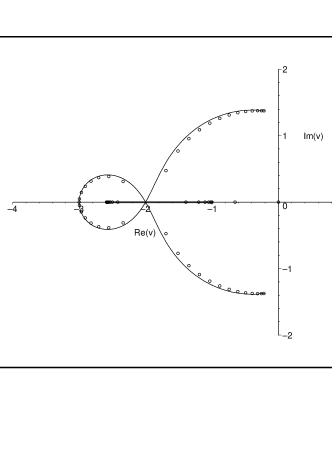
Figure 9: Locus ${\cal B}_{v}$ for the Potts model on a $2\times\infty$ strip of the triangular lattice with free boundary conditions and with $Q$ and $v$ satisfying eq. (5). Partition function zeros are shown for a free $2\times 20$ strip.

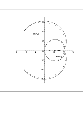
Figure 10: Locus ${\cal B}_{Q}$ for the Potts model on a $2\times\infty$ strip of the triangular lattice with free boundary conditions and with $Q$ and $v$ satisfying eq. (5). Partition function zeros are shown for a free $2\times 20$ strip.

In the limit $m\to\infty$, we find the locus ${\cal B}_{v}$ shown in Fig. 9 consisting of the union of (i) a curve that crosses the real $v$ axis at $v=-2$ (a multiple point on the curve) and $v=-3$ and has endpoints at the two complex-conjugate roots of the cubic factor in the square root in eq. (51), $v\simeq-0.206\pm 1.37i$ and (ii) a line segment on the real $v$ axis extending from $v=-1$ to $v\simeq-2.587$. These endpoints of the line segment are the other two zeros of the polynomial in the square root in eq. (51). This locus divides the complex $v$ plane into two regions. The image of this locus under the mapping (5), ${\cal B}_{Q}$, is shown in Fig. 10 and consists of the union of a closed curve passing through $Q=0$ and $Q=4$ with complex-conjugate arcs passing through $Q=4$ and terminating at endpoints $Q\simeq-4.38\pm 4.12i$, and a line segment on the real axis extending from $Q=2$ to $Q\simeq 2.762$. In Figs. 9 and 10 we also show zeros calculated for a long finite free $L_{y}=2$ strip of the triangular lattice. One sees again that these lie close to the asymptotic loci ${\cal B}_{v}$ and ${\cal B}_{Q}$, as one would expect for a long strip. There are also discrete zeros that do not lie on (or close to) the equimodular curves ${\cal B}$. We have already explained the origin of the zero at $(Q,v)=(0,0)$. In contrast to the situation with free strips of the square-lattice, where the zero at $v=0$ and its image at $Q=0$ were both isolated, here we find that for the free $L_{y}=2$ strip of the triangular-lattice (see Figs. 9, 10), there is an isolated zero at $v=0$, but because of the non one-to-one nature of the mapping (5), its image in the $Q$ plane is not isolated but rather is on ${\cal B}_{Q}$. We have also performed analogous studies of wider strips of the triangular lattice using the calculations of Ref. tt , and we find qualitatively similar results.

IV.3 Cyclic and Möbius

For cyclic boundary conditions we have $N_{Z,2,\lambda}=6$, $n_{Z}(2,0)=2$, $n_{Z}(2,1)=3$, $n_{Z}(2,2)=1$, just as in the square-lattice case. We calculated the general partition function $Z(t[2\times m],cyc.,Q,v)$ in Ref. ta , and this has the form of eq. (10) with $L_{y}=2$. Restricting $Q$ and $v$ to satisfy eq. (5), we obtain $\bar{\lambda}_{t,2,2}=1$, $\bar{\lambda}_{t,2,0,j}$ for $j=1,2$ given in eq. (51), and $\bar{\lambda}_{t,2,1,j}$ for $j=1,2,3$, which are solutions to the equation

$$\eta^{3}-(v+2)(3v+4)\eta^{2}+(v+2)(v+1)(3v^{2}+9v+4)\eta$$ (52)

(53)

$$-(v+1)^{2}(v^{2}+3v+1)^{2}=0\ .$$ (54)

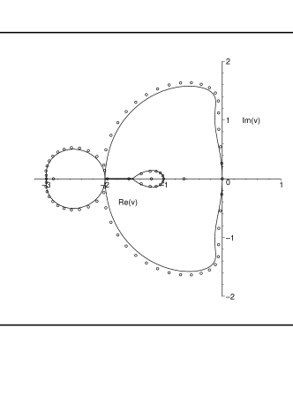
Figure 11: Locus ${\cal B}_{v}$ for the Potts model on a $2\times\infty$ strip of the triangular lattice with cyclic or Möbius boundary conditions and with $Q$ and $v$ satisfying eq. (5). Partition function zeros are shown for a cyclic $2\times 20$ strip.

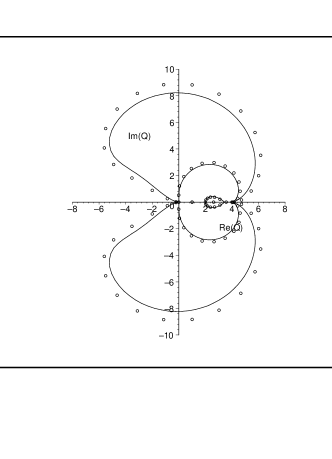
Figure 12: Locus ${\cal B}_{Q}$ for the Potts model on a $2\times\infty$ strip of the triangular lattice with cyclic or Möbius boundary conditions and with $Q$ and $v$ satisfying eq. (5). Partition function zeros are shown for a cyclic $2\times 20$ strip.

In the limit $m\to\infty$ for this cyclic strip (and for the same strip with Möbius boundary conditions), we find the locus ${\cal B}_{v}$ shown in Fig. 11 and the corresponding locus ${\cal B}_{Q}$ shown in Fig. 12. These loci consists of closed curves that intersect the real $v$ and $Q$ axis at the following points, where the value of $Q$ is the image of the value of $v$ under the mapping (5): (i) $v=0$ and $v=-3,\ \Rightarrow\ Q=Q_{2}=0$, (ii) $v=-1,\ \Rightarrow\ Q=Q_{4}=2$, and (iii) $v=-2,\ \Rightarrow\ Q=4$. The locus ${\cal B}_{v}$ also contains a line segment extending from $v\simeq-1.531$ to $v=-2$, and ${\cal B}_{Q}$ contains its image under the mapping (5), extending from $Q\simeq 3.44$ to $Q=4$.

The locus ${\cal B}_{v}$ separates the $v$ plane into four regions, as is evident in Fig. 11:

• the region including the intervals $v\geq 0$ and $v\leq-3$ on the real $v$ axis and extending to complex infinity, in which (with appropriate definition of the branch cuts associated with the square root in eq. (51)) $\bar{\lambda}_{t,2,0,1}$ is dominant,

• the region including the neighborhood to the left of $v=0$ and excluding the interior of the loop centered approximately around $v=-1.2$, in which one of the $\bar{\lambda}_{t,2,1,j}$’s is dominant,

• the region in the interior of the loop centered around $v=-1.2$, in which $\bar{\lambda}_{t,2,2}=1$ is dominant,

• the region including the interval that extends from $v=-2$ to $v=-3$, in which another $\bar{\lambda}_{t,2,1,j}$ is dominant.

We give some specific dominant eigenvalues at special points. At $v=0$, $\bar{\lambda}_{t,2,0,1}=(7+3\sqrt{5})/2$, equal in magnitude to the dominant $\bar{\lambda}_{t,2,1,j}$. At $v=-2$, all of the six $\bar{\lambda}_{t,2,d,j}$’s are equal in magnitude, and equal to unity. At $v=-3$, $|\bar{\lambda}_{t,2,0,j}|=2$ for $j=1,2$, and two of the $|\bar{\lambda}_{t,2,1,j}|=2$, while the third is equal in magnitude to 1.

Correspondingly, the locus ${\cal B}_{Q}$ divides the $Q$ plane into five regions:

• the region including the intervals $Q\geq 4$ and $Q\leq 0$ on the real $Q$ axis and extending to infinity, in which $\bar{\lambda}_{t,2,0,1}$ is dominant

• two complex-conjugate regions bounded at large $Q$ by curves that cross the imaginary axis at $Q\simeq\pm 8.23i$, in which one of the $\bar{\lambda}_{t,2,1,j}$’s is dominant

• the region including the interval $0\leq Q\leq 2$, in which another $\bar{\lambda}_{t,2,1,j}$ is dominant

• the region in the interior of the loop centered approximately around $Q=2.6$, in which $\bar{\lambda}_{t,2,2}=1$ is dominant

We have performed similar calculations for cyclic strips of the triangular lattice with greater widths, $L_{y}=3,4,5$. We find that ${\cal B}_{v}$ crosses the negative real axis at $v_{t2}(2\ell)$ for $1\leq\ell\leq L_{y}$, so that ${\cal B}_{Q}$ crosses the real axis at the image points under eq. (5), $Q_{2\ell}$. As with the cyclic square-lattice strips with widths $L_{y}\geq 3$, we find that the outermost curves on ${\cal B}_{Q}$ cross the negative real axis; for example, for $L_{y}=3$, such a crossing occurs at $Q\simeq-9.4$.

IV.4 Other Strips of the Triangular Lattice

We have also calculated the partition function and the resultant loci ${\cal B}_{v}$ and ${\cal B}_{Q}$ for strips of the triangular lattice with cylindrical and toroidal boundary conditions. A general feature that we find is that ${\cal B}_{v}$ passes through $v=-2$, and hence ${\cal B}_{Q}$ passes through $Q=4$. Other features depend on the specific boundary conditions and width. One property that we encounter is noncompactness of ${\cal B}_{v}$ and ${\cal B}_{Q}$ (as was the case with the $L_{y}=3$ toroidal strip of the square lattice and for cyclic self-dual strips of the square lattice qvsdg ).

V Strips of the Honeycomb Lattice

We first give a general solution for the three roots in $v$ of eq. (6) with $Q=Q_{r}$; in order of increasing value, these are

$$v_{hc1}(r)=-4\cos\Bigl{(}\frac{\pi}{r}\Bigr{)}\cos\biggl{[}\frac{\pi}{3}\Bigl{(}\frac{1}{r}-1\Bigr{)}\biggr{]}$$ (55)

$$v_{hc2}(r)=-4\cos\Bigl{(}\frac{\pi}{r}\Bigr{)}\cos\biggl{[}\frac{\pi}{3}\Bigl{(}\frac{1}{r}+1\Bigr{)}\biggr{]}$$ (56)

and

$$v_{hc3}(r)=4\cos\Bigl{(}\frac{\pi}{r}\Bigr{)}\cos\Bigl{(}\frac{\pi}{3r}\Bigr{)}\ .$$ (57)

As $r$ increases from 2 to $\infty$, and $Q_{r}$ thus increases from 0 to 4, (i) $v_{hc1}(r)$ decreases from 0 to a minimum of $-9/4$ at $r=\pi/\arcsin(\sqrt{10}/8)\simeq 7.73$ and then increases to $-2$; (ii) $v_{hc2}(r)$ decreases monotonically from 0 to $-2$; and (iii) $v_{hc3}(r)$, the physical root, increases monotonically from 0 to 4. As with the analogous expressions for the triangular lattice, it is straightforward to work out simpler expressions to which eqs. (55)-(57) reduce for special values of $r$; we omit the details here.

For this honeycomb lattice, substituting the value $v=-2$ into eq. (6) yields two solutions, $Q=2$ and $Q=4$. Using our general solutions for the partition functions $Z(hc[2\times m],free,Q,v)$ and $Z(hc[2\times m],cyc.,Q,v)$ in Ref. hca , we have checked that at $v=-2$, $Q=4$ there is degeneracy of dominant $\lambda$’s, so that these points are on the respective loci ${\cal B}_{v}$ and ${\cal B}_{Q}$. This property is thus similar to the feature that we have found for strips of the square and triangular lattices. For $L_{y}=2$ cyclic honeycomb-lattice strips we find that, in addition, the points $v=0$, $Q=Q_{2}=0$ and $v=-2$, $Q=Q_{4}=2$ are on the respective loci ${\cal B}_{v}$ and ${\cal B}_{Q}$. For the $L_{y}=3$ cyclic strips of this lattice, ${\cal B}_{v}$ contains these points and also $v_{hc1}(6)=-2\sqrt{3}\,\cos(5\pi/18)$, so that the image ${\cal B}_{Q}$ contains the point $Q=Q_{6}=3$. For all the strips of this lattice that we have studied, with $L_{y}$ up to $L_{y}=5$, we find that ${\cal B}_{v}$ crosses the real axis at $v=v_{hc1}(2\ell)$ for $\ell=1,\cdots,L_{y}$, so that ${\cal B}_{Q}$ crosses the real $Q$ axis at $Q_{2\ell}$ for $\ell=1,\cdots,L_{y}$.

VI Discussion

We remark on several features that are common to all of the strips of the three types of lattices that we have analyzed. These include the following:

• For all of the strips, including those of the square, triangular, and honeycomb lattices, that we have studied where nontrivial continuous accumulation loci are defined (thus excluding the $1\times m$ line graph with free boundary conditions), we find that ${\cal B}_{v}$ passes through $v=-2$ and ${\cal B}_{Q}$ passes through $Q=4$, which is the image of $v=-2$ under both of the mappings (4) and (5) and is a solution of eq. (6) with $v=-2$.

• For all of the cyclic (and equivalently, Möbius) strips that we have studied, besides the crossing at $Q=4$, ${\cal B}_{Q}$ crosses the real axis at

  $$Q=Q_{2\ell}\quad{\rm for}\ \ \ell=1,\cdots,L_{y}\ .$$ (58)

  We conjecture that this holds for arbitrarily large $L_{y}$. This locus can also cross the real axis at other points, such as the crossings on the negative real axis that we found for widths $L_{y}\geq 3$.

For the particular case of the cyclic square-lattice strips, these properties agree with a result in Ref. saleur2 , namely, that at $Q=Q_{2\ell}$, $|\lambda_{sq,L_{y},\ell,max}|=|\lambda_{sq,L_{y},\ell-1,max}|$, where $\lambda_{sq,L_{y},\ell,max}$ denotes the eigenvalue $\lambda_{sq,L_{y},\ell,j}$ of largest magnitude.

We also observed that the points $v=-2$ and $Q=4$ play a special role for self-dual strips of the square lattice in Ref. qvsdg . It is interesting that for self-dual cyclic square-lattice strips, in addition to the point $Q=4$, ${\cal B}_{Q}$ crosses the real axis at $Q_{2\ell+1}$ for $1\leq\ell\leq L_{y}$. This set of points is interleaved with those in eq. (58). As we have noted in Ref. qvsdg , these findings are in accord with the fact that the Potts model at the values $Q=Q_{r}$ has special properties, such as the feature that the Temperley-Lieb algebra is reducible at these values martinber ; saleur1 ; saleur2 ; ct . In Ref. qvsdg we compared our exact results for ${\cal B}$ on infinite-length, finite-width cyclic self-dual strips of the square lattice with calculations of partition function zeros for finite $L\times L$ sections of the square lattice with $Q=v^{2}$ in Ref. kc with the same boundary conditions. For finite lattice sections, there is, of course, no locus ${\cal B}_{Q}$ defined, and hence one is only able to make a rough comparison of patterns of zeros. In the calculation of zeros for the above-mentioned $L\times L$ section of the square lattice with cyclic self-dual boundary conditions, e.g., for $L=8$, a number of zeros in the $Q$ plane occur at or near to certain $Q_{r}$’s, and the zeros in the $v$ and $Q$ planes exhibit patterns suggesting the importance of the points $v=-2$ and $Q=4$. With our results in the present paper, we can extend this comparison. We see that the importance of $v=-2$ and $Q=4$ for the pattern of partition function zeros for $Q$ and $v$ satisfying the relation (4) generalizes to square-lattice strips with a variety of boundary conditions, not necessary self-dual. Indeed, going further, our results show that the features we have observed are true not just of the partition function on the square-lattice strips with $Q=v^{2}$, but also on strips of the triangular and honeycomb lattices with $Q$ and $v$ satisfying the analogous phase transition conditions (5) and (6). One interesting aspect of the findings in the present work and our Ref. qvsdg on infinite-length, finite-width strips is the special role of the value $Q=4$ for the loci ${\cal B}_{Q}$, which can make a connection with the locus ${\cal B}$ for the physical phase transition of the Potts model on two-dimensional lattices. In this context, we recall that the value $Q=4$ is the upper end of the interval $0\leq Q\leq 4$ for which the ferromagnetic Potts model has a second-order transition on two-dimensional lattices.

VII Conclusions

In conclusion, we have presented exact results for the continuous accumulation set ${\cal B}$ of the locus of zeros of the Potts model partition function for the infinite-length limits of strips of the square, triangular, and honeycomb lattices with various widths, a variety of boundary conditions, and $Q$ and $v$ restricted to satisfy the conditions (4), (5), and (6) for the ferromagnetic phase transition on the corresponding two-dimensional lattices. We have discussed some interesting general features of these loci.

VIII Acknowledgments

This research was partially supported by the Taiwan NSC grant NSC-94-2112-M-006-013 (S.-C.C.) and the U.S. NSF grant PHY-00-98527 (R.S.).

IX Appendix

In this Appendix we list the $v_{tj}(r)$ for $r=6$, 8, and 10, which are relevant to the analysis of the cyclic strips of the triangular lattice for widths up to $L_{y}=5$. From eqs. (37)-(39), we have

$$v_{tj}(6),\ j=1,2,3\quad\Longrightarrow\quad Q=Q_{6}=3$$ (59)

where r6

$$v_{t1}(6)=-1+2\cos(7\pi/9)\simeq-2.532089$$ (60)

$$v_{t2}(6)=-1+2\cos(5\pi/9)\simeq-1.347296$$ (61)

$$v_{t3}(6)=-1+2\cos(\pi/9)\simeq 0.879385$$ (62)

$$v_{tj}(8),\ j=1,2,3\quad\Longrightarrow\quad Q=Q_{8}=2+\sqrt{2}$$ (63)

where

$$v_{t1}(8)=-1-\sqrt{2}\simeq-2.414214$$ (64)

$$v_{t2}(8)=-1+\frac{1-\sqrt{3}}{\sqrt{2}}\simeq-1.517638$$ (65)

$$v_{t3}(8)=-1+\frac{1+\sqrt{3}}{\sqrt{2}}\simeq 0.931852$$ (66)

$$v_{tj}(10),\ j=1,2,3\quad\Longrightarrow\quad Q=Q_{10}=\frac{5+\sqrt{5}\,}{2}$$ (67)

where

$$v_{t1}(10)=\frac{1}{4}\biggl{(}-5+\sqrt{5}\,-\sqrt{30+6\sqrt{5}}\ \biggr{)}\simeq-2.338261$$ (68)

(69)

(70)

$$v_{t2}(10)=-\frac{(1+\sqrt{5}\,)}{2}\simeq-1.618034$$ (71)

$$v_{t3}(10)=\frac{1}{4}\biggl{(}-5+\sqrt{5}\,+\sqrt{30+6\sqrt{5}}\ \biggr{)}\simeq 0.956295$$ (72)

(73)

(74)

References

- (1) F. Y. Wu, Rev. Mod. Phys. 54, 235 (1982).
- (2) R. J. Baxter, Exactly Solved Models in Statistical Mechanics (Academic Press, New York, 1982).
- (3) P. Martin, Potts Models and Related Problems in Statistical Mechanics (World Scientific: Singapore, 1991).
- (4) S.-C. Chang and R. Shrock, cond-mat/0602178.
- (5) P. Kasteleyn and C. Fortuin, J. Phys. Soc. Jpn. 26 (Suppl.), 11 (1969); C. Fortuin and P. Kasteleyn, Physica 57, 536 (1972).
- (6) W. T. Tutte, J. Combin. Theory 2, 301 (1967); ibid. 9, 289 (1970).
- (7) W. T. Tutte, “Chromials”, in Lecture Notes in Mathematics, v. 411, p. 243 (1974); W. T. Tutte, Graph Theory, vol. 21 of Encyclopedia of Mathematics and Applications (Addison-Wesley, Menlo Park, 1984).
- (8) N. Biggs, Algebraic Graph Theory, 2nd ed. (Cambridge Univ. Press, Cambridge, 1993).
- (9) We note that in the application of the conditions for the Potts model on the two-dimensional lattices, the variable is normally fixed (to a non-negative integer) and one solves for the temperature-like variable . For each of the three lattices, although the equations (4)-(6) are nonlinear in , only one of the (two, for , three, for ) roots in is in the physical ferromagnetic range .
- (10) For a planar graph , the Tutte polynomial satisfies , where is the planar dual of . The self-duality of the square lattice is manifested in the fact that the condition is invariant under the interchange . The fact that the honeycomb lattice is the dual of the triangular lattice is manifested in the property that the conditions (t) and (hc) transform into each other under the interchange .
- (11) S. Beraha, J. Kahane, and N. Weiss, J. Combin. Theory B 27, 1 (1979); J. Combin. Theory B 28, 52 (1980).
- (12) H. Saleur, Commun. Math. Phys.132, 657 (1990).
- (13) H. Saleur, Nucl. Phys. B 360, 219 (1991).
- (14) S.-C. Chang and R. Shrock, Physica A 296, 131 (2001).
- (15) S.-C. Chang and R. Shrock, Physica A 296, 183 (2001).
- (16) R. Shrock, Physica A 283, 388 (2000).
- (17) S.-C. Chang and R. Shrock, Physica A 296, 234 (2001).
- (18) S.-C. Chang, J. Salas, and R. Shrock, J. Stat. Phys. 107, 1207 (2002).
- (19) S.-C. Chang and R. Shrock, Physica A 347, 314 (2005).
- (20) S.-C. Chang and R. Shrock, Physica A, in press (cond-mat/0506274).
- (21) S.-C. Chang and R. Shrock, Physica A 286, 189 (2000).
- (22) S.-C. Chang, J. Jacobsen, and J. Salas, and R. Shrock, J. Stat. Phys. 114, 763 (2004).
- (23) P. Martin, J. Phys. A 20, L399 (1987).
- (24) A related fact is that complex-temperature phase diagrams of the Potts model show special properties at . In addition to the trivial cases and and the exactly solvable Ising case , complex-temperature phase diagrams have been studied for various such as and in, e.g., Refs. martinbook , a -tt and chw -jrs . These studies are complementary to Refs. qvsdg ; kc and the present work in that and are kept as independent variables rather than being restricted to satisfy a condition such as one of eqs. (4)-(6).
- (25) C. N. Chen, C. K. Hu, and F. Y. Wu, Phys. Rev. Lett. 76, 169 (1996).
- (26) V. Matveev and R. Shrock, Phys. Rev. E 54, 6174 (1996).
- (27) H. Feldmann, R. Shrock, and S.-H. Tsai, Phys. Rev. E 57, 1335 (1998).
- (28) H. Feldmann, A. J. Guttmann, I. Jensen, R. Shrock, and S.-H. Tsai, J. Phys. A 31 2287 (1998).
- (29) S.-C. Chang and R. Shrock, Int. J. Mod. Phys. B 15, 443 (2001).
- (30) S.-C. Chang and R. Shrock, Phys. Rev. E 64, 066116 (2001).
- (31) J. Jacobsen, J.-F. Richard, and J. Salas, Nucl. Phys. B, to appear.
- (32) S.-Y. Kim and R. Creswick, Phys. Rev. E 63, 066107 (2001).
- (33) There are various equivalent ways to write the expressions for the roots of eqs. (5) and (6) with . For example, for , i.e., , the special cases of our general eqs. (37), (38), and (39) for , , are equivalent to eqs. (2.14), (2.13), and (2.12) of Ref. p2 and the special cases of our general eqs. (55), (56), and (57) for , , are equivalent to eqs. (3.5), (3.4), and (3.3) of Ref. p .