Phase diagrams of one-dimensional Bose-Fermi mixtures of ultra-cold atoms

Abstract

We study the quantum phase diagrams of Bose-Fermi mixtures of ultracold atoms confined to one dimension in an optical lattice. For systems with incommensurate densities, various quantum phases, e.g. charge/spin density waves, pairing, phase separation, and the Wigner crystal, are found to be dominant in different parameter regimes within a bosonization approach. The structure of the phase diagram leads us to propose that the system is best understood as a Luttinger liquid of polarons (i.e. atoms of one species surrounded by screening clouds of the other species). Special fillings, half-filling for fermions and unit filling for bosons, and the resulting gapped phases are also discussed, as well as the properties of the polarons and the experimental realization of these phases.

I Introduction

In recent years the experimental control of trapped ultracold atoms has evolved to a level that allows to probe sophisticated many-body effects, in particular the regime of strong correlations. One of the most prominent achievements, the realization of the superfluid to Mott-insulator transition of bosonic atoms in an optical lattice Jaksch ; MISF , triggered both experimental and theoretical research into quantum phase transitions of ultracold atoms in optical lattices. The advances in trapping and cooling techniques, as well as the manipulation of atom-atom interactions by Feshbach resonances feshbach , created the possibility to study many-body systems in the quantum degenerate regime in a widely tunable environment. Of particular interest are those systems that resemble solid-state systems, for example, mixtures of ultra-cold bosonic and fermionic atoms bfm , which have recently become accessible through the development of sympathetic cooling sympathetic_cooling . On the theoretical side several phenomena have been proposed in the literature like pairing of fermions pairing , formation of composite particles composite , spontaneous breaking of translational symmetry in optical lattices burnett ; xCDW . However, the approach used in most of these studies, which relied on integrating out the bosonic degrees of freedom and then using a mean-field approach to investigate many-body states pairing , becomes unreliable in the regime of strong interactions, in particular, in low-dimensional systems. A non-perturbative and beyond-mean-field investigation is therefore of high interest.

In one-dimensional (1D) systems, on the other hand, many physical problems can be solved exactly by various mathematical methods because of the restricted phase space and higher order geometric symmetry. One of the most successful examples is the Luttinger liquid model for 1D electron systems review . The pioneering work of Tomonaga tomonaga , Luttinger luttinger and Haldane haldane ; haldane_bf along with many others has produced an essentially complete understanding of the low energy physics of these systems (within the so called bosonization approach). Recently these theoretical methods were also applied to systems of ultra-cold atoms cazalilla ; ho ; mathey , where the bosonic or fermionic atoms are confined in a highly enlongated magnetic-optical trap potential and approach an ideal 1D or quasi-1D system. Such 1D or quasi-1D enlongated trap potentials can be easily prepared either in a traditional magnetic-optical trap 1D_tradition , magnetic waveguides on microchips microchip , or in an anisotropic optical lattice 1Doptical_lattice . However, since there is no true long-range order in a homogeneous 1D system in the thermodynamic limit, the one-dimensional “quantum phases” we will refer to in this paper are actually understood in the sense of quasi-long-range order (QLRO), i.e. the correlation function of a given order parameter ($O(x)$) has an algebraic decay at zero temperature, $\langle O(x)O(0)\rangle\sim|x|^{-2+\alpha}$, where $\langle\cdots\rangle$ is the ground state average, $x$ is the distance, and $\alpha$ is the scaling exponent associated with that order parameter. As a result, the dominant quantum phase is determined by the largest scaling exponent $\alpha>0$ (i.e. the slowest algebraic decay of the correlation functions of a given order parameter). At the phase boundaries that appear in the phase diagrams in this paper, the scaling exponent of the corresponding type of order becomes positive, i.e. the corresponding susceptibility switches from finite to divergent.

In this paper we extend and elaborate on our previous work mathey on one-dimensional (1D) Bose-Fermi mixtures. We give a detailed derivation of the effective low-energy Hamiltonian of a 1D BFM within a bosonization approach haldane_bf ; cazalilla . After diagonalizing this Hamiltonian we calculate the long-distance behavior of the single particle correlation functions. We introduce a fermionic polaron ($f$-P) operator, constructed out of a fermionic operator with a screening cloud of bosonic atoms, and determine the single-particle correlation function, as well as the correlation functions of various order parameters, which are used to construct the phase diagram. For a BFM of one species of fermions with one species of bosons, we find a charge density wave (CDW) phase that competes with the pairing phase of fermionic polarons ($f$-PP), giving a complete description of the system as a Luttinger liquid of polarons. When the boson-fermion interaction strength is stronger than a critical value, we observe the Wentzel-Bardeen instability (WB) region, where the BFM undergoes phase separation (PS) for repulsive interaction or collapse (CL) for attractive interaction.

We also study several special cases when the density of the fermions or the bosons is commensurate with the lattice period. The low energy effective Hamiltonian of these cases cannot be diagonalized but instead has to be studied by using a renormalization group (RG) method. We obtain a charge gapped phase for half-filling of the fermions and for unit filling of the bosons, and study how these phases are affected by the presence of the other species.

We also apply the bosonization method in an analogous approach to spinful fermions mixed with a single species of bosonic atoms. We find a rich quantum phase diagram, including spin/charge density waves (SDW/CDW), triplet/singlet fermionic polaron pairing, and a regime showing the Wentzel-Bardeen instability. The similarity with the known phase diagram of 1D interacting electronic systems review , again suggests that a 1D BFM is best understood as a Luttinger liquid of polarons. We also discuss the close relationship between the polarons constructed in the bosonization approach in this paper and the canonical polaron transformation usually applied in solid state physics.

This paper is organized as follows: In Section II, we present the microscopic description of a BFM and its bosonized representation. In Section III, we calculate the scaling exponents of single particle correlation functions as well as the correlation functions of various order parameters. Quantum phase diagrams obtained by comparing these different scaling exponents are presented in the anti-adiabatic regime, i.e. the phonon velocity is much larger than the Fermi velocity. In Section IV, we present the results of two commensurate filling regimes: half-filling of fermions, and unit filling of bosons. In Section V, we study a BFM of spinful fermions with $SU(2)$-symmetry and determine the rich phase diagram of this system. In Section VI, we discuss questions regarding the experimental realization of the quantum phase diagrams presented in this paper, and we summarize our results in Section VII. In Appendix A we give a more technical derivation of the scaling exponents of various operators. In Appendix B we discuss the notion of polarons used in this paper, and compare it to the those used in solid state systems. The effects of a local impurity in the system are discussed in Appendix C.

II Bosonized Hamiltonian and Exact Diagonalization

In this section we derive and discuss the effective low energy Hamiltonian of a 1D BFM in the limit of large bosonic filling ($\nu_{b}\gg\nu_{f}$, where $\nu_{b/f}$ is the bosonic/fermionic filling fraction) and fast bosons ($v_{b}\gg v_{f}$, where $v_{b}$ is the bosonic phonon velocity, and $v_{f}$ is the Fermi velocity). We also mention how this study can be extended to the regime of comparable velocities ($v_{f}\sim v_{b}$).

We consider a BFM in an anisotropic optical lattice, where the lattice strengths for bosons ($b$) and fermions ($f$) can be expressed as $V_{b(f)}({\bf r})=\sum_{\alpha=x,y,z}V_{b(f),\alpha}\sin^{2}(k_{l}r_{\alpha})$ with $k_{l}=2\pi/\lambda$ being the laser wavevector and $\lambda$ being the wavevector of the laser fields. Throughout this paper we will use $\lambda/2=1$ (which corresponds to the lattice constant of the optical lattice) as the natural length scale. In order to create an effectively 1D lattice, we consider $V_{b(f),||}\ll V_{b(f),\perp}$, where $V_{b(f),||}=V_{b(f),x}$ is the lattice strength along the longitudinal direction and $V_{b(f),\perp}=V_{b(f),y}=V_{b(f),z}$ is along the transverse direction, so that the single particle tunneling between each 1D tube is strongly surpressed. We note that independent tuning of the optical lattice strength for these two species of atoms can be achieved even when only a single pair of lasers provides the standing beam in each direction. This can be done due to the fact that the strength of an optical lattice for a given atom is proportional to $\Omega_{R}^{2}/(\nu-\Delta E)$ bec_book , where $\Omega_{R}$ is the Rabi frequency (which is proportional to the laser intensity), $\nu$ is the laser frequency, and $\Delta E$ is the resonance energy of that atom — therefore for two different species of atoms (different $\Delta E$), their effective lattice strengths can be tuned independently over a wide range, by simultaneously changing the laser intensities via $\Omega_{R}$ and the laser frequency $\nu$.

II.1 Hamiltonian

For sufficiently strong optical potentials the microscopic Hamiltonian is given by a single band Hubbard model Jaksch :

$$H = -\sum_{\langle ij\rangle}\left(t_{b}b_{i}^{\dagger}b_{j}+t_{f}f_{i}^{\dagger}f_{j}\right)-\sum_{i}\left(\mu_{f}n_{f,i}+\mu_{b}n_{b,i}\right)$$ (1)

$$+\frac{U_{b}}{2}\sum_{i}n_{b,i}(n_{b,i}-1)+U_{bf}\sum_{i}n_{b,i}n_{f,i},$$

where $n_{b,i}\equiv b^{\dagger}_{i}b_{i}$ and $n_{f,i}\equiv f^{\dagger}_{i}f_{i}$ are the boson and fermion density operators, and $\mu_{b/f}$ are their chemical potentials. The tunneling amplitudes $t_{f/b}$, and the particle interactions $U_{b}$ and $U_{bf}$ can be calculated from the lattice strengths and the $s$-wave scattering lengths:

$$t_{b(f)} = (4/\sqrt{\pi})\bar{V}_{b(f),\parallel}^{3/4}E_{b(f)}\exp(-2\bar{V}_{b(f),\parallel}^{1/2})$$ (2)

$$U_{b} = (8/\pi)^{1/2}(2\pi a_{bb}/\lambda)E_{b}(\bar{V}_{b,\parallel}\bar{V}_{b,\perp}^{2})^{1/4}$$ (3)

$$U_{bf} = (8/\pi)^{1/2}(2\pi a_{bf}/\lambda)E_{bf}(\bar{V}_{bf,\parallel}\bar{V}_{bf,\perp}^{2})^{1/4}$$ (4)

We defined $\bar{V}_{b(f),\parallel/\perp}=V_{b(f),\parallel/\perp}/E_{b(f)}$ and $\bar{V}_{bf,\parallel(\perp)}=(4\bar{V}_{b,\parallel(\perp)}\bar{V}_{f,\parallel(\perp)})/((\bar{V}_{b,\parallel(\perp)}^{1/2}+\bar{V}_{f,\parallel(\perp)}^{1/2})^{2})$. $E_{b(f)}=(2\pi/\lambda)^{2}/2m_{b(f)}$ are the recoil energies of the two atomic species, and $E_{bf}$ is given by $E_{bf}=(m_{b}+m_{f})/4m_{b}m_{f}(2\pi/\lambda)^{2}$.

For the convenience of the subsequent discussion we also give the Hamiltonian in momentum space:

$$H = H_{b}^{(0)}+H_{f}^{(0)}+H_{bf}$$ (5)

Here, $H_{b}^{(0)}$ refers to the bosonic sector without the coupling to the fermions, and is given by:

$$H_{b}^{(0)} = \sum_{k}(\epsilon_{b,k}-\mu_{b})b_{k}^{\dagger}b_{k}+\frac{U_{b}}{2L}\sum\rho_{b,k}^{\dagger}\rho_{b,k}$$ (6)

$L$ is the 1D system length. $\epsilon_{b,k}$ is given by $\epsilon_{b,k}=-2t_{b}\cos k$, and $\rho_{b,k}$ is defined as $\rho_{b,k}=\sum_{p}b_{p+k}^{\dagger}b_{p}$. The free fermionic sector - without the coupling to the bosons - is given by:

$$H_{f}^{(0)} = \sum_{k}(\epsilon_{f,k}-\mu_{f})f_{k}^{\dagger}f_{k}$$ (7)

where $\epsilon_{f,k}$ is given by $\epsilon_{f,k}=-2t_{f}\cos k$. The interaction between these two sectors can be written as:

$$H_{bf} = \frac{U_{bf}}{L}\sum_{k}\rho_{f,k}^{\dagger}\rho_{b,k}$$ (8)

with $\rho_{f,k}=\sum_{p}f_{p+k}^{\dagger}f_{p}$.

II.2 Low energy effective Hamiltonian

To determine the effective low energy Hamiltonian, we first consider the effective Hamiltonian of weakly interacting bosons, $H_{b}^{(0)}$, without coupling to the fermions. Following the standard Bogoliubov transformation bec_book ; bogoliubove , we obtain the following effective low-energy Hamiltonian for the bosonic sector:

$$H_{b}^{(0)} \rightarrow \sum_{k\neq 0}\omega_{b,k}\beta_{k}^{\dagger}\beta_{k},$$ (9)

where the $\beta_{k}$ are the Bogoliubov phonon operators and $\omega_{b,k}=\sqrt{(\epsilon_{b,k}-\epsilon_{b,0})(\epsilon_{b,k}-\epsilon_{b,0}+2U_{b}\nu_{b})}$ is the phonon dispersion. The phonon operators $\beta_{k}$ are related to the original boson operators by $\beta_{k}=u_{k}b_{k}-v_{k}b_{-k}^{\dagger}$, where $u_{k}^{2}=1+v_{k}^{2}=(\epsilon_{b,k}-\epsilon_{b,0}+U_{b}\nu_{b}+\omega_{b,k})/2\omega_{b,k}$ and $u_{k}v_{k}=-U_{b}\nu_{b}/2\omega_{b,k}$ are the coefficients of the Bogoliubov transformation bec_book . We note that, although this tranformation is considered as a treatment of the quadratic fluctuations around a meanfield approximation, it is still applicable to 1D systems where no true condensate exists even at zero temperature (see [castin, ]). In the long wavelength limit, we have $\omega_{b,k}=v_{b}|k|$, where $v_{b}=\sqrt{2t_{b}U_{b}\nu_{b}}$ is the phonon velocity.

For the fermionic sector we proceed along the lines of the Luttinger liquid formalism, established in solid state physics tomonaga ; luttinger ; haldane ; review . We linearize the noninteracting fermion band energy around the two Fermi points (at $\pm k_{f}$, with $k_{f}$ being the Fermi wavevector, $k_{f}=\pi\nu_{f}$), and split the fermion operator into a right ($R$) and a left ($L$) moving channel. One can show that such a linearized band Luttinger model luttinger is effectively equivalent to a bilinear bosonic Hamiltonian in the low energy limit:

$$H_{f}^{(0)} \rightarrow \sum_{k\neq 0}v_{f}|k|B^{\dagger}_{k}B_{k},$$ (10)

where $B_{k}$ is a bosonic (density) operator defined as $B_{k}\equiv i\sqrt{\frac{2\pi}{kL}}\sum_{p}f^{\dagger}_{R,k+p}f_{R,p}$ for $k>0$ and $B_{k}\equiv-i\sqrt{\frac{2\pi}{|k|L}}\sum_{p}f^{\dagger}_{L,k+p}f_{L,p}$ for $k<0$. $f_{R/L,k}$ are the right/left movers and

$$v_{f} = 2t_{f}\sin(k_{f})$$ (11)

is the Fermi velocity.

Finally we will address the interaction between the bosonic and the fermionic atoms. In the low-energy limit, there are two kinds of scattering to be considered. One is the scattering by exchanging small momentum in both the fermionic and the bosonic sector. The other one is the scattering by exchanging a momentum of $2k_{f}$ to reverse the direction of a fermion moving in 1D. For the first term, only the long wavelength density fluctuations are important so the corresponding interaction can be expressed by the same transformation used above:

$$H_{bf}^{(1)} \rightarrow \sum_{k\neq 0}g|k|(\beta_{k}^{\dagger}+\beta_{-k})(B_{k}+B_{-k}^{\dagger}).$$ (12)

where $g$ and $K_{b}$ are given by

$$g = U_{bf}\sqrt{K_{b}}/2\pi$$ (13)

$$K_{b} = \pi\sqrt{2t_{b}\nu_{b}/U_{b}}$$ (14)

$K_{b}$ is the Luttinger parameter for bosons as will be discussed further in the next section.

For the second case, low energy excitations occur in the backward scattering channel, and therefore cannot be included in Eq. (12), shown above. Such a backward scattering term, in general, leads to a non-linear and non-diagonalizable term in the Hamiltonian. We therefore consider a certain parameter regime in which the backward scattering term becomes tractable. In this and the next section (III), we will consider a BFM with large bosonic filling (i.e. $\nu_{b}\gg\nu_{f}$), and fast boson limit (i.e. $v_{b}\gg v_{f}$). Experimentally, this limit can be achieved by choosing $t_{b}\gg t_{f}$, and $\nu_{b}\approx 1-3$, for typical atomic interactions. For simplicity, we will also assume that both the bosonic and the fermionic filling fraction are not commensurate to the lattice period or to each other. We will show that the Hamiltonian of such a system can be solved exactly even in the presence of backward scattering.

In the limit of large bosonic filling and fast boson velocity, it is easy to see that the backward scattering of fermions is mainly provided by the forward scattering of bosons (because $2k_{f}=2\pi\nu_{f}\ll 2k_{b}=2\pi\nu_{b}$), so that the effective interaction Hamiltonian in this channel can be written as

$$H_{bf}^{(2)} \rightarrow \frac{1}{\sqrt{L}}\sum_{|k|\sim 2k_{f}}g_{2k_{f}}(\beta_{k}^{\dagger}+\beta_{-k})\sum_{p}f^{\dagger}_{p+k}f_{p}$$ (15)

where the coupling is given by $g_{k}=U_{bf}[\nu_{b}(\epsilon_{b,k}-\epsilon_{b,0})/2\pi\omega_{b,k}]^{1/2}$. The next step is to separate the non-interacting phonon field, Eq. (9), into a low energy and high energy part, $H=\sum_{|k|<k_{f}}\omega_{k}\beta_{k}^{\dagger}\beta_{k}+\sum_{|k|>k_{f}}\omega_{k}\beta_{k}^{\dagger}\beta_{k}$, and then integrate out the latter for $|k|\sim 2k_{f}$, together with the backward scattering term in Eq. (15). Since we assume $v_{b}\gg v_{f}$, we can obtain an effective interaction between fermions within an instaneous approximation. After some algebra, we can obtain such an effective fermion-fermion interaction to be:

$$H_{f}^{(1)} = -\frac{1}{L}\frac{g_{2k_{f}}^{2}}{\omega_{2k_{f}}}\sum_{|k|\sim 2k_{f}}\sum_{p}f^{\dagger}_{p}f_{p+k}\sum_{q}f^{\dagger}_{q+k}f_{q}$$ (16)

$$= \frac{1}{L}\frac{g_{2k_{f}}^{2}}{\omega_{2k_{f}}}\sum_{\alpha=\pm}\sum_{k\sim 2\alpha k_{f}}\sum_{p,q\sim-\alpha k_{f}}f^{\dagger}_{p}f_{q}f^{\dagger}_{q+k}f_{p+k}$$

$$= \frac{1}{L}\frac{g_{2k_{f}}^{2}}{\omega_{2k_{f}}}\sum_{k^{\prime}\sim 0}\left[n_{R,k^{\prime}}n_{L,k^{\prime}}+n_{L,k^{\prime}}n_{R,k^{\prime}}\right]$$

where $n_{R/L,k}\equiv\sum_{p}f^{\dagger}_{R/L,p+k}f_{R/L,p}$ is the density operator for the right/left moving electrons. We therefore find that the original backward scattering obtained by integrating out the boson field now becomes a forward scattering term with repulsive interaction between the left and right movers. Therefore we can apply the bosonization approach for Luttinger liquids used in Eq. (10) and obtain

$$H_{f}^{(1)} = \sum_{k\sim 0}G|k|(B_{k}B_{-k}+B_{k}^{\dagger}B_{-k}^{\dagger})$$ (17)

where

$$G = \frac{g_{2k_{f}}^{2}}{\omega_{2k_{f}}}.$$ (18)

Therefore the sum of the terms given in Eq. (9), (10), (12) and (17) is our final effective low energy Hamiltonian within the limit of large bosonic filling and fast boson velocity. The total Hamiltonian then becomes:

$$H = \sum_{k\neq 0}\omega_{b,k}\beta_{k}^{\dagger}\beta_{k}+\sum_{k\neq 0}v_{f}|k|B^{\dagger}_{k}B_{k}$$ (19)

$$+\sum_{k\neq 0}g|k|(\beta_{k}^{\dagger}+\beta_{-k})(B_{k}+B_{-k}^{\dagger})$$

$$+\sum_{k\sim 0}G|k|(B_{k}B_{-k}+B_{k}^{\dagger}B_{-k}^{\dagger}),$$

which is bilinear in two different bosonic operators and therefore can be diagonalized exactly. For the convenience of later discussion and calculating the correlation functions, in the next section we will use Haldane’s bosonization representation to express the effective Hamiltonian shown above.

II.3 Effective Hamiltonian in Haldane’s bosonization representation

We now bosonize both fermions and bosons on equal footing by introducing the phase and density fluctuation operators haldane_bf ; cazalilla through the definitions:

$$f(x) = \left[\nu_{f}+\Pi_{f}\right]^{1/2}\sum_{m=-\infty}^{\infty}e^{(2m+1)i\Theta_{f}}e^{i\Phi_{f}}$$ (20)

$$b(x) = \left[\nu_{b}+\Pi_{b}\right]^{1/2}\sum_{m=-\infty}^{\infty}e^{2mi\Theta_{b}}e^{i\Phi_{b}}$$ (21)

where we use $x$ to denote a continuous coordinate if there is no lattice potential in the longitudinal direction or a discrete coordinate in the presence of a lattice. $\Pi_{b/f}(x)$ and $\Phi_{b/f}(x)$ are respectively the density and phase fluctuations with $\Theta_{b/f}\equiv\pi\nu_{b/f}x+\pi\int^{x}dy\Pi_{b/f}(y)$ accounting for the discreteness of atoms along the 1D direction. The density and phase fluctuations satisfy the commutation relations:

$$\left[\Pi_{b/f}(x),\Phi_{b/f}(x^{\prime})\right]=i\delta(x-x^{\prime}).$$ (22)

The advantage of using the density-phase fluctuation representation for boson-fermion mixture is that it treats the fermions and bosons in the same way. We do not have to use a Bogoliubov transformation for the bosonic field and a Luttinger liquid formalism for fermions separately as has been done above. As has been established in the literature (e.g. haldane_bf ; cazalilla ), the effective low energy Hamiltonian of the bosonic and the fermionic sector can be written in terms of the fields $\Pi_{b/f}$ and $\Phi_{b,f}$ as:

$$H_{b}^{(0)} = \frac{v_{b}}{2}\int dx\left[\frac{K_{b}}{\pi}\left(\partial_{x}\Phi_{b}\right)^{2}+\frac{\pi}{K_{b}}\Pi_{b}^{2}\right]$$ (23)

$$H_{f}^{(0)} = \frac{v_{f}}{2}\int dx\left[\frac{K_{f}}{\pi}\left(\partial_{x}\Phi_{f}\right)^{2}+\frac{\pi}{K_{f}}\Pi_{f}^{2}\right],$$ (24)

where we have $K_{f}=1$ due to the absence of $s$-wave short-range interaction between fermionic atoms. Note that for intermediate values of the bosonic interaction $U_{b}$, the phonon velocity $v_{b}$ and the Luttinger exponent $K_{b}$ are renormalized by higher order terms. They can be obtained by solving the model exactly via Bethe-ansatz and are found to be very well approximated by

$$v_{b} = \frac{\nu_{s}}{m^{\ast}_{b}}\sqrt{\gamma}\left(1-\frac{\sqrt{\gamma}}{2\pi}\right)^{1/2}$$ (25)

and

$$K_{b} = \frac{\pi}{\sqrt{\gamma}}\left(1-\frac{\sqrt{\gamma}}{2\pi}\right)^{-1/2},$$ (26)

where $m^{\ast}_{b}$ is the effective boson mass in the presence of the lattice potential stringari and $\nu_{s}\sim\nu_{b}$ is the superfluid fraction. $\gamma\equiv m^{\ast}_{b}U_{b}/\nu_{s}$ is a dimensionless parameter, characterizing the interaction strength of the 1D boson system. To leading order in the interaction (in the weakly interacting limit $\gamma\rightarrow 0$), $v_{b}$ and $K_{b}$ are the same as before.

The density and phase fluctuations, defined in Eqs. (20) and (21), can be related to the bosonic operators $\beta_{k}$ and $B_{k}$ by (see cazalilla )

$$\Pi_{b}(x) = \frac{1}{2\pi}\sum_{k\neq 0}\sqrt{\frac{2\pi K_{b}}{L|k|}}\,{\rm sgn}(k)e^{ikx}\left(\beta_{k}+\beta_{-k}^{\dagger}\right)$$ (27)

$$\Phi_{b}(x) = \frac{1}{2}\sum_{k\neq 0}\sqrt{\frac{2\pi}{L|k|K_{b}}}\,{\rm sgn}(k)e^{ikx}\left(\beta_{k}-\beta_{-k}^{\dagger}\right),$$ (28)

$$\Pi_{f}(x) = \frac{1}{2\pi}\sum_{k\neq 0}\sqrt{\frac{2\pi K_{f}}{L|k|}}\,{\rm sgn}(k)e^{ikx}\left(B_{k}+B_{-k}^{\dagger}\right)$$ (29)

$$\Phi_{f}(x) = \frac{1}{2\pi}\sum_{k\neq 0}\sqrt{\frac{2\pi}{L|k|K_{f}}}\,{\rm sgn}(k)e^{ikx}\left(B_{k}-B_{-k}^{\dagger}\right).$$ (30)

which can also be seen by comparing Eqs. (23)-(24) with Eqs. (9)-(10)

The long wavelength limit of the boson-fermion interaction and the backward scattering Hamiltonian shown in Eqs. (12) and (17) can also be expressed in terms of the density and phase fluctuations operators as follows:

$$H_{bf}^{(1)} = U_{bf}\int dx\,\Pi_{b}\,\Pi_{f}$$ (31)

$$H_{f}^{(1)} = \frac{2G}{2\pi}\int dx\left[\pi^{2}\Pi_{f}^{2}-(\partial_{x}\Phi_{f})^{2}\right].$$ (32)

Therefore the total low-energy effective Hamiltonian is given by the sum of Eqs. (23), (24), (31), and (32):

$$H_{\rm eff} = H_{f}^{(0)}+H_{b}^{(0)}+H_{bf}^{(1)}+H_{f}^{(1)}$$ (33)

which can be diagonalized easily as described below.

Before solving the effective Hamiltonian, we note that similar problems have been investigated in the context of electron-phonon interactions in one-dimensional solid state physics in the literature, both with voit_phonon ; egger or without Engelsberg ; meden backward scattering of electrons. In the previous studies, the backward scattering of fermions was treated in bosonized form before integrating out the phonon field. The resulting effective interaction obtained after integrating out the high energy phonon field is of the form voit_phonon

$$H_{f}^{(1)}\propto\int\!\!\!\int d^{2}{\bf r}d^{2}{\bf r}^{\prime}D_{0}({\bf r}-{\bf r}^{\prime})\cos\left[2\Theta_{f}({\bf r})\right]\cos\left[2\Theta_{f}({\bf r}^{\prime})\right],$$

(34)

where ${\bf r}=(x,v_{f}\tau)$ is a space vector in 1+1 dimension and $D_{0}({\bf r}-{\bf r}^{\prime})$ is the phonon propagator. (Note that the symbol of density and phase fluctuations used in this paper and in Eq. (34) is different from Ref. voit_phonon .) The instantaneous approximation of the phonon propagator is given by $D_{0}({\bf r}-{\bf r}^{\prime})\propto\delta({\bf r}-{\bf r}^{\prime})$. However, Eq. (34) does not seem to reduce to a bilinear term as shown Eq. (32). Such superficial disagreement can be resolved by taking the normal ordered form of $\cos(2\Theta)$ carefully, as treated by Sankar in Ref. sankar . In our treatment we keep the fermionic form after integrating out the phonon field and rearranging the order of fermions before using bosonization, which is a technically simpler and unambiguous procedure. It shows that within the instantaneous limit the 1D BFM system (and the related electron-phonon system) can be described by a bilinear bosonized Hamiltonian, which then can be diagonalized exactly, even in the presence of backward scattering.

We note that the generic form of the effective Hamiltonian (33) extends beyond the parameter regime assumed in this section. If we drop the assumption of fast bosons ($v_{b}\gg v_{f}$), and rather assume these velocities to be comparable, a renormalization argument of the type presented in voit_phonon shows that the resulting Hamiltonian can also be written as (33). Then, however, the expressions for the effective parameters shown in this section would not hold anymore, and would need to be replaced by parameters resulting from the RG flow.

II.4 Diagonalized Hamiltonian

We now go on to diagonalize the full effective low energy Hamiltonian (Eq. (33)) by using the following linear transformation Engelsberg :

$$\Pi_{b}=\delta_{1}\Pi_{A}+\delta_{2}\Pi_{a}, \Phi_{b}=\epsilon_{1}\Phi_{A}+\epsilon_{2}\Phi_{a},$$

$$\Pi_{f}=\beta_{1}\Pi_{A}+\beta_{2}\Pi_{a}, \Phi_{f}=\gamma_{1}\Phi_{A}+\gamma_{2}\Phi_{a},$$ (35)

where $\Pi_{A/a}$ and $\Phi_{A/a}$ are the density and phase operators of the two eigenmodes, and the coefficients are given by:

$$\begin{array}[]{ll}\beta_{1}=e^{\theta}\sqrt{\frac{\tilde{v}_{f}}{v_{A}}}\cos\psi&\beta_{2}=e^{\theta}\sqrt{\frac{\tilde{v}_{f}}{v_{a}}}\sin\psi\\ \gamma_{1}=e^{-\theta}\sqrt{\frac{v_{A}}{\tilde{v}_{f}}}\cos\psi&\gamma_{2}=e^{-\theta}\sqrt{\frac{v_{a}}{\tilde{v}_{f}}}\sin\psi\\ \delta_{1}=-e^{\phi}\sqrt{\frac{v_{b}}{v_{A}}}\sin\psi&\delta_{2}=e^{\phi}\sqrt{\frac{v_{b}}{v_{a}}}\cos\psi\\ \epsilon_{1}=-e^{-\phi}\sqrt{\frac{v_{A}}{v_{b}}}\sin\psi&\epsilon_{2}=e^{-\phi}\sqrt{\frac{v_{a}}{v_{b}}}\cos\psi.\end{array}$$ (40)

Here we have $e^{\theta}=((v_{f}-2G)/(v_{f}+2G))^{1/4}$, $e^{\phi}=\sqrt{K_{b}}$, and $\tan 2\psi=4\tilde{g}(v_{b}\tilde{v}_{f})^{1/2}/(v_{b}^{2}-\tilde{v}_{f}^{2})$. The diagonalized Hamiltonian

$$H = \frac{1}{2}\sum_{j=a,A}v_{j}\int dx\left[\pi\Pi_{j}(x)^{2}+\frac{1}{\pi}\left(\partial_{x}\Phi_{j}(x)\right)^{2}\right]$$ (41)

has the eigenmode velocities, $v_{A}$ and $v_{a}$, given by

$$v_{a/A}^{2} = \frac{1}{2}(v_{b}^{2}+\tilde{v}_{f}^{2})\pm\frac{1}{2}\sqrt{(v_{b}^{2}-\tilde{v}_{f}^{2})^{2}+16\tilde{g}^{2}v_{b}\tilde{v}_{f}},$$ (42)

where $\tilde{v}_{f}\equiv(v_{f}^{2}-4G^{2})^{1/2}$ and $\tilde{g}\equiv g\,e^{\theta}$, $e^{\theta}$ is given by $e^{\theta}=((v_{f}-2G)/(v_{f}+2G))^{1/4}$.

From Eq. (42) we note that when the fermion-phonon coupling $g$ (proportional to $U_{bf}$) becomes sufficiently strong, the eigenmode velocity $v_{A}$ becomes imaginary, indicating an instability of the system to phase separation (PS) or collapse (CL), depending on the sign of $U_{bf}$ ho ; instability . This is the so-called Wentzel-Bardeen instability, and has been studied before in 1D electron-phonon systems ho

III Scaling exponents and quantum phase diagrams

In this section, we will calculate the scaling exponents of various quasi-long-range order parameters to construct the quantum phase diagram. The diagonalized form of the Hamiltonian, which we presented in Section II.4, allows an exact calculation of all correlation functions (see Appendix A). For the later discussion, we define the following “scaling exponents” to mimic the ones in standard single component bosonic cazalilla or fermionic systems review :

$$K_{\beta} \equiv \beta_{1}^{2}+\beta_{2}^{2},\ \ \ K_{\gamma}^{-1}\equiv\gamma_{1}^{2}+\gamma_{2}^{2}$$ (43)

$$K_{\delta} \equiv \delta_{1}^{2}+\delta_{2}^{2},\ \ \ K_{\epsilon}^{-1}\equiv\epsilon_{1}^{2}+\epsilon_{2}^{2}$$ (44)

$$K_{\beta\delta} \equiv \beta_{1}\delta_{1}+\beta_{2}\delta_{2}\ \ \ K_{\gamma\epsilon}^{-1}\equiv\gamma_{1}\epsilon_{1}+\gamma_{2}\epsilon_{2}.$$ (45)

Note that since $v_{a}>v_{A}$ according to Eq. (42), we have $K_{\beta\delta}<0$ and $K_{\gamma\epsilon}^{-1}>0$. From Eq. (35) it is apparent that $K_{\beta}$ and $K_{\gamma}^{-1}$ are the scaling exponent associated with the fermion density and phase fluctuations, respectively, and $K_{\delta}$ and $K_{\epsilon}^{-1}$ are associated with the boson density and phase fluctuations. $K_{\beta\delta}$ and $K^{-1}_{\gamma\epsilon}$ are related to fluctuations of mixed components, and appear in the scaling exponents of products of fermionic and bosonic operators.

III.1 Single particle correlation functions and polaron operators

In this section we consider the single-particle correlation functions of the system. For the bare bosonic and fermionic particles we find $\langle b(x)b^{\dagger}(0)\rangle\sim|x|^{-\frac{1}{2}K_{\epsilon}^{-1}}$ and $\langle f(x)f^{\dagger}(0)\rangle\sim\cos(k_{f}x)|x|^{-\frac{1}{2}(K_{\beta}+K_{\gamma}^{-1})}$, as discussed in Appendix A. The scaling exponents that appear in these correlation functions have been renormalized by the coupling between the bosons and the fermions.

Motivated by the polaronic effects in electron-phonon systems, we next consider a class of operators that seems to be most appropiate as the elementary operators of the system. In BFMs each atom will repel (attract) the atoms of the other species in its vicinity, due to their mutual interaction, resulting in a reduced (enhanced) density around that atom. To describe particles dressed with screening clouds of the other species we introduce the following composite operators (polarons):

$$\tilde{f}_{\lambda}(x)\equiv e^{-i\lambda\Phi_{b}(x)}f(x),$$ (46)

$$\tilde{b}_{\eta}(x)\equiv e^{-i\eta\Phi_{f}(x)}b(x),$$ (47)

with $\lambda$ and $\eta$ being real numbers, describing the size of the screening cloud. The correlation functions of these new fermionic and bosonic operators can be calculated to be (cp. Appendix A)

$$\langle\tilde{f}_{\lambda}(x)\tilde{f}^{\dagger}_{\lambda}(0)\rangle \sim \cos(k_{f}x)|x|^{-\frac{1}{2}(K_{\beta}+K_{\gamma}^{-1}-2\lambda K_{\gamma\epsilon}^{-1}+\lambda^{2}K_{\epsilon}^{-1})}$$

$$\langle\tilde{b}_{\eta}(x)\tilde{b}^{\dagger}_{\eta}(0)\rangle \sim |x|^{-\frac{1}{2}(K_{\epsilon}^{-1}+\eta^{2}K_{\gamma}^{-1}-2\eta K_{\gamma\epsilon}^{-1})}.$$ (49)

Treating $\lambda$ and $\eta$ as variational parameters, we observe that the exponents of the correlation functions are minimized (i.e. the correlation functions have the slowest decay at long distances) by taking $\lambda_{c}=K_{\epsilon}/K_{\gamma\epsilon}$ and $\eta_{c}=K_{\gamma}/K_{\gamma\epsilon}$. To gain some insight into the quantity $\lambda_{c}$ we consider the limit of weak boson-fermion interaction ($U_{bf}\rightarrow 0$) and obtain approximately $\lambda_{c}\sim U_{bf}/U_{b}$ (for further discussion, see Appendix B). This result can be interpreted by a simple density counting argument as follows: we imagine a single fermionic atom interacting with $-\lambda$ bosons in its vicinity. The potential energy of such a configuration can be estimated as $-U_{bf}\lambda+U_{b}\lambda^{2}/2$, which is minimized by taking $\lambda=U_{bf}/U_{b}$. Since the polaronic cloud size is not a well-defined quantum number, $\lambda_{c}$ and $\eta_{c}$ need not be integers and depend on the boson-fermion interaction strength continuously.

Taking the optimal values of $\lambda_{c}$ and $\eta_{c}$ in Eqs. (46)-(47) and using the following two identities: $K_{\beta}^{-1}=K_{\gamma}^{-1}-K_{\epsilon}K_{\gamma\epsilon}^{-2}$ and $K_{\delta}^{-1}=K_{\epsilon}^{-1}-K_{\gamma}K_{\gamma\epsilon}^{-2}$, we can show that

$$\langle\tilde{f}_{\lambda_{c}}(x)\tilde{f}^{\dagger}_{\lambda_{c}}(0)\rangle \sim \cos(k_{f}x)|x|^{-\frac{1}{2}(K_{\beta}+K_{\beta}^{-1})}$$ (50)

$$\langle\tilde{b}_{\eta_{c}}(x)\tilde{b}^{\dagger}_{\eta_{c}}(0)\rangle \sim |x|^{-\frac{1}{2}K_{\delta}^{-1}}.$$ (51)

In other words, the long-distance (low energy) behavior of both the fermionic-polaron ($f$-P, defined in Eq. (46) with $\lambda=\lambda_{c}$) and the bosonic-polaron ($b$-P, defined in Eq. (47) with $\eta=\eta_{c}$) are characterized by a single scaling parameter, $K_{\beta}$ and $K_{\delta}$, respectively, in contrast to the scaling behavior of the bare atoms. As we will see in the next section, the many body correlation functions of operators composed of such fermionic polarons also scale with the same single parameter, $K_{\beta}$, leading to the conclusion that the 1D BFM system is best understood as a Luttinger liquid of polarons, instead of bare fermions.

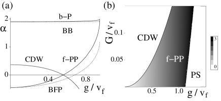
Figure 1: (a) Scaling exponents of various order parameters as a function of longitudinal FP coupling $g$ for a BFM with spinless fermions. Parameters are chosen to be: $v_{b}/v_{f}=3$, $K_{b}=5$ and $G/v_{f}=0.1$. Different curves correspond to the $2k_{f}$–CDW, $f$-polaron pairing field ($f$-PP), bare fermion pairing field (BFP), $b$-polaron operator ($b$-P), and bare boson operator (BB). Note that operators constructed with polarons (i.e. $b$-P and $f$-PP) always have larger exponents than their counterparts constructed with bare atoms. (b) Global phase diagram of the same system in terms of effective forward scattering between fermions, $G$ and the fermion-phonon coupling $g$ for $v_{b}/v_{f}=5$ and $K_{b}=10$. Three different phases, CDW, $f$-PP, and phase separation (PS) are dominant successively from weak to strong fermion-phonon coupling strength.

III.2 Correlation functions of order parameters

It is well established that there is no true off-diagonal long range order in 1D systems, due to strong fluctuations. Therefore, in this paper, the ground state is characterized by the order parameter that has the slowest long distance decay of the correlation function review , i.e. in the sense of QLRO. Transforming to momentum-energy space, this is equivalent to finding the most divergent susceptibility in the low temperature limit: if, at $T=0$, the correlation function of a certain order parameter $O(x)$ decays as $\langle O(x)O^{\dagger}(0)\rangle\sim 1/|x|^{2-\alpha}$ for large $x$, the finite $T$ susceptibility will diverge as $\chi(T)\sim 1/T^{\alpha}$. Here we defined the scaling exponent $\alpha$, which is positive for a quasi long range ordered state (i.e. $\chi(T)$ diverges for $T\rightarrow 0$), and negative if no such order is present. Across a phase boundary the susceptibility will switch from finite to divergent. Since we are interested here in the limit of high phonon velocity ($v_{b}\gg v_{f}$), only the fermionic degrees of freedom need to be considered for the low-energy (long-distance) behavior of the correlation functions. The bosonic sector is always assumed to be in a quasi-condensate state. (We will relax these assumptions below.)

Similar to a LL of spinless fermions, we first consider the order parameters of the CDW phase, defined as $O_{CDW}=f^{\dagger}_{L}(x)f_{R}(x)$, and of the $p$-wave pairing phase, given by $O_{BFP}=f_{L}(x)f_{R}(x)$, where the abbreviation BFP stands for bare fermion pairing. The scaling exponents for the CDW and the BFP phase can be calculated (see Appendix A) to be:

$$\alpha_{CDW} = 2-2K_{\beta}$$ (52)

$$\alpha_{BFP} = 2-2K^{-1}_{\gamma}$$ (53)

In Fig. 1 (a), we show the calculated scaling exponents for CDW and BFP phases as a function of the long-wavelength fermion-phonon coupling strength $g$, which is proportional to $U_{bf}$. The other parameters are given by $K_{b}=5$, $v_{b}/v_{f}=3$, and $G/v_{f}=0.1$. One can see that CDW ordering becomes dominant ($\alpha_{CDW}>0$) for $g/v_{f}<0.55$, while bare fermion pairing is dominant ($\alpha_{BFP}>0$) when $g/v_{f}>0.65$. In the intermediate regime ($0.55<g/v_{f}<0.65$) none of these two phases have quasi long range order, and therefore one might conclude that in this regime the system displays a metallic phase. A similar result has been discussed in the context of 1D electron-phonon systems, voit_phonon ; egger ; martin .

However, as mentioned in our earlier publication mathey , the above analysis is incomplete. An indication for this is given by how a single impurity potential affects the transport of the 1D BFM (see Appendix C). Following the renormalization group analysis by Kane and Fisher kane , we show that a single weak impurity potential is relevant when $\alpha_{CDW}=2-2K_{\beta}>0$ and becomes irrelevant whenever the system is outside the CDW regime, i.e. when $\alpha_{CDW}=2-2K_{\beta}<0$. This result is inconsistent with the previous CDW-metal-BFP scenario, because a metallic state would not be insensitive to an impurity potential in 1D. More precisely, the fact that the impurity potential becomes irrelevant even outside the BFP phase indicates that there is another superfluid-like ordering, which cannot be described by the pairing of bare fermions only.

Above observation motivates a further search for the appropiate order parameters. Among the many types of operators that can be considered, we find that the operator $O_{f-PP}=\tilde{f}_{L,\lambda_{c}}(x)\tilde{f}_{R,\lambda_{c}}(x)$, which describes a $p$-wave fermionic polaron pairing phase ($f$-PP), shows dominant scaling outside of the CDW regime. In Fig. 2 we give an illustration of the two phases that occur in BFMs with spinless fermions.

As shown in Appendix A, the scaling exponent of the fermionic polaron pairing phase can be calculated to be:

$$\alpha_{f-PP} = 2-2\left[\lambda^{2}_{c}K_{\epsilon}^{-1}+K_{\gamma}^{-1}-2\lambda_{c}K_{\gamma\epsilon}^{-1}\right]$$ (54)

$$= 2-2K_{\beta}^{-1},$$

where we used the same polarization parameter $\lambda_{c}$ as in the previous section, and the same algebraic relation between the scaling quantities as for the derivation of (50). Note that the expression (54) is dual to the scaling of the CDW operator, Eq. (52), and, hence, both the CDW phase and the $f$-polaron phase are governed by a single Luttinger parameter, $K_{\beta}$, which also appears in the single particle correlation function of $f$-polarons as shown in Eq. (50). The fact that the scaling exponents (50), (52) and (54) are the ones of a Luttinger liquid of 1D fermion with parameter $K_{\beta}$ indicates that the 1D BFM system should be understood as a Luttinger liquid of polarons. We note that $\tilde{f}^{\dagger}_{L,\lambda_{c}}\tilde{f}_{R,\lambda_{c}}=f^{\dagger}_{L,\lambda_{c}}f_{R,\lambda_{c}}$, as can be seen from the definition of $\tilde{f}$, Eq. (46). Therefore, the scaling exponent of $O_{CDW}$ is not affected by the screening cloud. In Fig. 1(a) we also show the scaling exponent of the new type of order parameter, $O_{f-PP}$. We note that $\alpha_{f-PP}$ is always larger than $\alpha_{BFP}$, showing that BFP cannot be the most dominant quantum phase in the whole parameter regime of a BFM. Furthermore, the scaling exponents shown in Fig. 1(a) demonstrate that divergencies of the CDW and $f$-PP susceptibilities are mutually exclusive and cover the entire phase diagram up to the phase separation (PS) regime, which can also been seen directly from the scaling exponents in Eqs. (52) and (54). This explains why a single impurity can be irrelavant when the system is in the regime between the CDW phase and the BFP phase, as discussed above.

In Fig. 2 we show a schematic representation of a CDW and an $f$-PP phase. In Fig. 1(b) we show a global phase diagram of a BFM by considering the FP coupling ($g$) and the effective fermion-fermion interaction ($G$) as independent variables. The shading density indicates the strength of the phonon cloud of the $f$-polaron pairing phase, $2\lambda_{c}$. We find that for a fixed effective backward scattering between fermions, i.e. $G=$constant, CDW phase, $f$-PP phase and phase separation regimes become dominant successively when the long-wavelength fermion-phonon coupling ($g$) is increased.

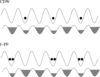
Figure 2: Illustration of the two phases that occur in a BFM with spinless fermions, CDW and $f$-PP. In the CDW phase the system develops a $2k_{f}$ density modulation in both the fermionic and the bosonic liquid. In the $f$-PP phase, fermionic polarons pair up and form a superfluid state.

III.3 Polaronic effects on bosons

The polaronic construction, demonstrated and discussed in the previous sections for the fermionic atoms, can also be done for the bosonic atoms, see Eq. (47). In Fig. 1(a), we also show the calculated scaling exponent of the bare boson condensation field, $O_{BB}(x)=b(x)$, and that of the bosonic polaron ($b$-polaron) condensation field, $O_{b-P}(x)=\tilde{b}(x)$. In one dimensional systems, the elementary excitations of the fermions are Luttinger bosons review , which can provide the bosonic screening clouds around the bosonic atoms, leading to a higher scaling exponent than the bare bosons as shown in Fig. 1(a). However, in the fast boson limit ($v_{b}\gg v_{f}$) that we consider here, the dressing of the bosonic atoms is very weak (i.e. $\alpha_{BB}\approx\alpha_{b-P}$) unless the system is close to the phase separation region.

III.4 Phase diagram in terms of experimental parameters

In the last sections we derived and discussed the $T=0$-phase diagram of BFMs. We will now give two plots of the same phase diagram in terms of parameters that are experimentally more accessible. In the first example (depicted in Fig. 3 (a)), we assume that the lattice strengths $V_{f/b,\perp/\|}$ can be tuned independently, and we keep the densities $\nu_{f}$ and $\nu_{b}$, and the boson-boson scattering length $a_{bb}$ constant. We now vary the boson-fermion scattering length $a_{bf}$ and the lattice strength $V_{b,\|}$ of the laser that is parallel to the system direction and couples to the bosons. This lattice strength mostly affects the bosonic tunneling $t_{b}$: For small $V_{b,\|}$, the tunneling amplitude is large, and therefore the phonons are fast. For large $V_{b,\|}$ the phonons are slow and the system develops CDW QLRO. For large values of $a_{bf}$ the system experiences the Wentzel-Bardeen instability, as shown in Fig. 1 b).

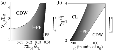
Figure 3: (a) Phase diagram for a mixture of bosonic and spinless fermionic atoms in a 1D optical lattice, for the first example discussed in Section III.4. Shading in the $f$-PP phase describes the strength of the bosonic screening cloud ($2\lambda_{c}$, see Eq.(46)) around a pair of fermions. $\lambda_{L}$ and $E_{R}$ are the lattice period and recoil energy, respectively. Other parameters used for this figure are (see text for notations): $\nu_{b}=4$, $\nu_{f}=0.5$, $V_{b,\perp}=V_{f,\perp}=20E_{R}$, $V_{f,\|}=2E_{R}$, boson-boson scattering length $a_{bb}=0.01\lambda_{L}$. (b) Phase diagram for a mixture of bosonic and spinless fermionic atoms in a 1D optical lattice, for the second example in Section III.4. Shading in the $f$-PP phase describes the absolute value of the strength of the bosonic screening cloud ($|2\lambda_{c}|$) around a pair of fermions. Other parameters used for this figure are (see text for notations): $\nu_{b}=3$, $\nu_{f}=0.2$, $V_{f,\perp}/E_{f}=20$, $V_{b,\perp}/E_{b}=1.65V_{f,\perp}/E_{f}$, boson-boson scattering length $a_{bb}=100a_{0}$, where $a_{0}$ is the Bohr radius.

As a second example we will now discuss a ⁸⁷Rb-⁴⁰K mixture in an anisotropic optical lattice created by a set of Nd:YAG lasers. In Fig. 3 (b) we show a phase diagram for a mixture of bosons and spinless fermions as a function of the scattering length between bosons and fermions ($a_{bf}$ (in units of $a_{0}$)) and the strength of the longitudinal optical lattice for fermionic atoms ($V_{f,\|}/E_{f}$). We assume that the lasers are far detuned from the transition energies, and that the optical lattices for the bosons and the fermions are created by the same set of lasers. In this set-up, the bosonic and fermionic lattice strengths are now constrained to the ratio: $V_{b,\|/(\perp)}/E_{b}=1.65V_{f,\|/(\perp)}/E_{f}$ for a laser wavelength of $830nm$ [hmoritz, ]. We chose negative values for the boson-fermion scattering length, because for most combinations of hyperfine states the scattering length between ⁸⁷Rb and ⁴⁰K is negative. Due to the different scaling of $v_{b}$ and $v_{f}$ with $V_{b,\|}/E_{b}$ and $V_{f,\|}/E_{f}$ the ratio of $v_{b}/v_{f}$ varies going along the vertical axis. The lower portion of the diagram corresponds to slower bosons (compared to the fermions) the upper part to faster bosons. For relatively weak boson-fermion interactions and strong confinement the system is again in the CDW phase, in which the densities of fermions and bosons have a $2k_{f}$-modulation. In the case of very strong boson-fermion interactions the system is again unstable to to a Wentzel-Bardeen instability, which now leads to collapse (CL) ho ; instability , rather than phase separation. The two regimes are separated by an $f$-PP phase with an increasing value of the polarization parameter $\lambda_{c}$ for stronger interaction.

IV Phase diagrams in other parameter regimes

In the previous two sections we have considered BFMs in the limit of large bosonic filling ($\nu_{b}\gg\nu_{f}$) and fast bosons ($v_{b}\gg v_{f}$). We also assumed that both the fermionic filling and the bosonic filling are incommensurate to each other and to the lattice, so that higher harmonics of the bosonization representation could be neglected. We will now consider two cases in which these assumptions are relaxed in different ways: In section IV.1, we consider a BFM with fermions at half-filling. At this particular fermionic filling, phonon-induced Umklapp scattering can open a charge gap. In Sec. IV.2 we consider the case when the boson filling fraction is unity, so that the system can undergo a Mott insulator transition. A further discussion of commensurate mixtures is given in commix .

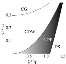
Figure 4: Phase diagram of a BFM with spinless fermions at half-filling. All parameters are as in Fig.1 b. For large $G$ a charge gap (CG) appears due to the Umklapp scattering.

IV.1 Charge-gapped phase for half-filling of the fermions

In this section we still assume the system to be in the regime of slow fermions ($v_{f}\ll v_{b}$) and large bosonic filling ($\nu_{b}\gg\nu_{f}$), but the fermionic filling is set to be at half-filling, i.e. $\nu_{f}=1/2$. In this situation, the derivation given in Eq. (16), leading to the backscattering term Eq. (32), has to include Umklapp scattering, which involves a momentum transfer of $4k_{f}=4\pi\nu_{f}=2\pi$. Similar to the derivation of Eq. (32), Umklapp scattering can be obtained to be:

$$H_{uk} = -\frac{1}{L}\frac{g_{2k_{f}}^{2}}{\omega_{2k_{f}}}\sum_{\alpha=\pm}\sum_{k\sim 2\alpha k_{f}}\sum_{p,q\sim\alpha k_{f}}f^{\dagger}_{p+k}f_{p}f^{\dagger}_{q+k}f_{q}.$$ (55)

In bosonized representation, this expression becomes:

$$H_{uk} = -\frac{2g_{3}}{(2\pi\alpha)^{2}}\int dx\cos\left[4\theta_{f}(x)\right].$$ (56)

$g_{3}$ is the Umklapp parameter given by $g_{3}=\frac{g_{2k_{f}}^{2}}{\omega_{2k_{f}}}$, which is equal to the backscattering parameter $G$. Since this is a nonlinear term that cannot be diagonalized, we use a scaling argument to study its effect. Such a renormalization flow argument at tree-level corresponds to a systematic expansion around $g_{3}=0$. The scaling dimension of this term is $4K_{\beta}$, so the flow equation for $g_{3}$ is given by:

$$\frac{dg_{3}}{dl} = (2-4K_{\beta})g_{3}$$ (57)

Therefore, the Umklapp term is relevant for $K_{\beta}<1/2$. When $g_{3}$ becomes relevant, the fermion excitations become gapped due to the strong repulsion mediated by the $2k_{f}$-phonons. As indicated in Fig. 4, we find that such a charge gap (CG) opens in the large $G$ regime.

Figure 5: Phase diagram of a BFM with unit bosonic filling. For small $K_{b}$ and small $g$ the bosons undergo a Mott insulator transition. In this diagram we only indicated the phases of the bosons. The fermions will be in an $f$-PP phase throughout the diagram.

IV.2 Mott insulator transition for bosons at unit filling

In this section we determine how the Mott insulator (MI) transition in the bosonic sector is affected by the presence of the incommensurate fermionic liquid. However, the results of this section equally apply to a boson-boson mixture because the dynamical properties of fermions and bosons in 1D are very similar. The starting point for our discussion is not the single band Hubbard model (Eq. 1), but a continuous 1D system, to which we add a weak $2k_{b}$-periodic external potential:

$$H_{2k_{b}} = \int dxV_{2k_{b}}\cos 2\theta_{b}.$$ (58)

So the entire system is described by

$$H = H^{(0)}_{b}+H^{(0)}_{f}+H_{bf}^{(1)}+H_{2k_{b}}$$ (59)

For simplicity we neglect the fermion backward scattering term. We again use a scaling argument to determine the effect of the non-linear term (58). This term has a scaling dimension of $K_{\delta}$, and its flow equation is therefore given by:

$$\frac{dV_{2k_{b}}}{dl} = (2-K_{\delta})V_{2k_{b}}$$ (60)

The condition for the Mott insulator transition is therefore $K_{\delta}<2$. Since we always have $K_{\delta}>K_{b}$, the presence of the other atomic species tends to ’melt’ the Mott insulator. This can also be seen in Fig. 5: For $g=0$ we obtain a Mott insulator for $K_{b}<2$ and a superfluid for $K_{b}>2$. However, when we increase the fermion-phonon coupling $g$ the Mott insulator regime shrinks and even vanishes entirely before phase separation is reached. This is reasonable because the coupling to the second species of atoms induces an attractive interaction, which tends to decrease the tendency of the bosons to form a Mott insulator at unit filling.

V Spinful system

In this section we consider BFMs that have fermions with two internal hyperfine states. We assume the fermionic sector to be $SU(2)$ symmetric, that is, the two Fermi velocities and their filling fraction are equal, as well as their coupling to the bosonic atoms. We again consider the limit of fast bosons, $v_{b}\gg v_{f}$.

V.1 Hamiltonian

Analogous to the Hamiltonian of a BFM with spinless fermions, Eq. (33), we describe the two internal states with the fields $\Theta_{\uparrow,\downarrow}$ and $\Phi_{\uparrow,\downarrow}$. In terms of these fields, the fermionic sector is described by a Hamiltonian of the form:

$$H_{f}^{0} = \int dx\Big{\{}\sum_{i=\uparrow,\downarrow}\frac{v_{f}}{2}\Big{[}\frac{K_{f}}{\pi}\left(\partial_{x}\Phi_{i}\right)^{2}+\frac{\pi}{K_{f}}\Pi_{i}^{2}\Big{]}$$ (61)

$$+U_{\uparrow\downarrow}\Pi_{\uparrow}\Pi_{\downarrow}+\frac{2U_{\uparrow\downarrow}}{(2\pi\alpha)^{2}}\cos(2\theta_{\uparrow}-2\theta_{\downarrow})\Big{\}},$$

where $\alpha{\rightarrow}0^{+}$ is the intrinsic cut-off of the bosonization representation. The parameter $U_{\uparrow\downarrow}$ describes the $s$-wave scattering between two spin states. The last term is the backscattering term, which occurs because the two fermionic spin states have equal filling. The bosonic sector is of the same form as before:

$$H_{b}^{0} = \frac{v_{b}}{2}\int dx\left[\frac{K_{b}}{\pi}\left(\partial_{x}\Phi_{b}\right)^{2}+\frac{\pi}{K_{b}}\Pi_{b}^{2}\right]$$ (62)

Analogous to Eq. (31), the long wavelength density fluctuations of the fermions and the bosons are linearly coupled:

$$H_{bf}^{(1)} = U_{bf}\int dx\Pi_{b}(\Pi_{\uparrow}+\Pi_{\downarrow}).$$ (63)

Finally, we also integrate out the $2k_{f}$-phonons of the bosonic superfluid, leading to the following interaction between fermions:

$$H_{f}^{1} = \sum_{i=\uparrow,\downarrow}\frac{2G}{2\pi}\int dx\left[\pi^{2}\Pi_{i}^{2}-(\partial_{x}\Phi_{i})^{2}\right]$$ (64)

$$-\frac{8\pi G}{(2\pi\alpha)^{2}}\int dx\cos\left(2\theta_{\uparrow}-2\theta_{\downarrow}\right)$$

The total low-energy Hamiltonian is then given by:

$$H = H_{f}^{0}+H_{b}^{0}+H_{bf}^{(1)}+H_{f}^{1},$$ (65)

which can be separated into spin and charge sectors, $H=H_{\rho}+H_{\sigma}$, by introducing the following linear combinations:

$$\Theta_{\rho/\sigma}=\frac{1}{\sqrt{2}}(\Theta_{\uparrow}\pm\Theta_{\downarrow}), \Phi_{\rho/\sigma}=\frac{1}{\sqrt{2}}(\Phi_{\uparrow}\pm\Phi_{\downarrow})$$ (66)

Note that $H_{\rho}$ coupled to the bosonic field is of the same form as a BFM with spinless fermions that we discussed earlier and can be diagonalized by a rotation similar to Eq. (35).

$$\Pi_{b}=\delta_{1}\Pi_{A}+\delta_{2}\Pi_{a}, \Phi_{b}=\epsilon_{1}\Phi_{A}+\epsilon_{2}\Phi_{a},$$

$$\Pi_{\rho}=\beta_{1}\Pi_{A}+\beta_{2}\Pi_{a}, \Phi_{\rho}=\gamma_{1}\Phi_{A}+\gamma_{2}\Phi_{a},$$ (67)

The diagonalized Hamiltonian of the charge sector has the same form as (41):

$$H_{\rho} = \frac{1}{2}\sum_{j=a,A}v_{j}\int dx\left[\pi\Pi_{j}(x)^{2}+\frac{1}{\pi}\left(\partial_{x}\Phi_{j}(x)\right)^{2}\right]$$ (68)

and, similarly, the eigenmode velocities, $v_{A}$ and $v_{a}$, are of the same form as (42):

$$v_{a/A}^{2} = \frac{1}{2}(v_{b}^{2}+v_{\rho}^{2})\pm\frac{1}{2}\sqrt{(v_{b}^{2}-v_{\rho}^{2})^{2}+16\tilde{g}_{\rho}^{2}v_{b}v_{\rho}},$$ (69)

where we defined $v_{\rho}\equiv(\tilde{v}_{\rho}^{2}-4G_{\rho}^{2})^{1/2}$ and $\tilde{g}_{\rho}\equiv g_{\rho}\,e^{\theta}$, with $e^{\theta}=((\tilde{v}_{\rho}-2G_{\rho})/(\tilde{v}_{\rho}+2G_{\rho}))^{1/4}$, $g_{\rho}$ by $g_{\rho}=\sqrt{2}g$. $\tilde{v}_{\rho}$ is given by $\tilde{v}_{\rho}=v_{f}+G$, $G_{\rho}=G+G_{\uparrow\downarrow}/2$. $G_{{\uparrow}{\downarrow}}$ is given by $G_{{\uparrow}{\downarrow}}=U_{{\uparrow}{\downarrow}}/2\pi$. All of these parameters and expressions can be immediately obtained by transferring the results from the spinless BFM case.

The quadratic part of the spin part of the Hamiltonian can be diagonalized by using

$$\Pi_{\sigma}=\sqrt{K_{\sigma}}\tilde{\Pi}_{\sigma}, \Phi_{\sigma}=1/\sqrt{K_{\sigma}}\tilde{\Phi}_{\sigma},$$ (70)

where $\sqrt{K_{\sigma}}\equiv e^{\phi_{\sigma}}$ and $\tanh 2\phi_{\sigma}=-2G_{\sigma}/\tilde{v}_{\sigma}$, with $\tilde{v}_{\sigma}=v_{f}-G_{\uparrow\downarrow}$, $G_{\sigma}=G-G_{\uparrow\downarrow}/2$ and $v_{\sigma}=\sqrt{\tilde{v}^{2}_{\sigma}-4G_{\sigma}^{2}}$. The transformed spin sector then becomes a sine-Gordon model,

$$H_{\sigma} = \frac{1}{2}v_{\sigma}\int dx\left[\pi\Pi_{\sigma}(x)^{2}+\frac{1}{\pi}\left(\partial_{x}\Phi_{\sigma}(x)\right)^{2}\right]$$ (71)

$$+\frac{2g_{1\perp}}{(2\pi\alpha)^{2}}\int dx\cos\left(\sqrt{8K_{\sigma}}\Theta_{\sigma}\right).$$

Here, $g_{1\perp}=U_{\uparrow\downarrow}-4\pi G$ is the effective backward scattering amplitude for fermions.

V.2 Renormalization flow

Figure 6: Linearized renormalization flow of the parameters $g_{1,\perp}$ and $K_{\sigma}$ in the vicinity of the SU(2) symmetric fixed point at $g_{1,\perp}=0$ and $K_{\sigma}=1$. Systems with SU(2) symmetry are forced to be on the separatrix from the upper right quadrant to the lower left quadrant. If the initial parameters of such a system correspond to a point in the upper right quadrant the system flows to the non-interacting, SU(2) symmetric fixed point at the origin. For initial parameters in the lower left quadrant the system flows towards a strongly interacting fixed point and opens a spin gap.

In this section, we deal with the spin Hamiltonian by performing an RG calculation, similar to the calculation in section IV. As discussed in review , and as is well-established in the literature, the RG flow at one-loop is given by:

$$\frac{dK_{\sigma}}{dl} = -\frac{K_{\sigma}^{2}}{2}\Big{(}\frac{g_{1,\perp}}{\pi v_{\sigma}}\Big{)}^{2}$$ (72)

$$\frac{dg_{1,\perp}}{dl} = (2-2K_{\sigma})g_{1,\perp}$$ (73)

These equations are a systematic expansion around the non-interacting fixed point at $g_{1,\perp}=0$ and $K_{\sigma}=1$. In Fig. 6, we show the linearized flow generated by these equations, in the vicinity of this fixed point. For $K_{\sigma}>1$, the parameters of the system flow towards the fixed point $(g_{1,\perp}=0,K_{\sigma}=1)$, whereas for $K_{\sigma}<1$, they flow towards the strong coupling fixed point $(g_{1,\perp}\rightarrow\pm\infty,K_{\sigma}=0)$. The nature of spin excitations of the ground state follows from the well known properties of the sine-Gordon model for SU(2) symmetry: When the initial $g_{1\perp}$ is positive the system has gapless spin excitations, i.e. $g_{1\perp}{\rightarrow}0$ and $K_{\sigma}{\rightarrow}1$, and when the initial $g_{1\perp}$ is negative the system has a spin gap, i.e. $g_{1\perp}{\rightarrow}-\infty$ and $K_{\sigma}{\rightarrow}0$.

V.3 Scaling exponents

Now we will determine the scaling exponents of the order parameters that can show QLRO in the phase diagram. The order parameters of a standard SU(2) symmetric LL of fermions are the charge density wave (CDW), spin density wave (SDW), singlet and triplet pairing (of bare fermions), and Wigner crystal (WC) operator. When such a system is coupled to a bosonic superfluid we again need to replace the pairing of bare fermions by pairing of polarons (analogous to Section III, see also Appendix A). First we consider the $2k_{f}$-mode of the CDW operator ($O_{CDW}=\sum_{s}f_{s,L}^{\dagger}f_{s,R}$) and of the SDW operator ($O_{SDW}=\sum_{s,s^{\prime}}f_{s,L}^{\dagger}\hat{\sigma}_{s,s^{\prime}}f_{s^{\prime},R}$). In bosonized form these correspond to $O_{CDW,2k_{f}}\sim\exp[\sqrt{2}i\Theta_{\rho}+\sqrt{2}i\Theta_{\sigma}]$ and $O_{SDW,2k_{f}}\sim\exp[\sqrt{2}i\Theta_{\rho}+\sqrt{2}i\Phi_{\sigma}]$. Their scaling exponents are given by

$$\alpha_{CDW} = 2-K_{\beta}-K_{\sigma}$$ (74)

$$\alpha_{SDW} = 2-K_{\beta}-K_{\sigma}^{-1}$$ (75)

For the polaron pairing phase, both singlet (SPP, $O_{SPP}=\tilde{f}_{\uparrow,L}\tilde{f}_{\downarrow,R}-\tilde{f}_{\downarrow,L}\tilde{f}_{\uparrow,R}$) and triplet (TPP, $O_{TPP}=\tilde{f}_{\uparrow,L}\tilde{f}_{\uparrow,R}$) pairing needs to be considered. In bosonized form, these operators are given by $O_{SPP,k=0}\sim\exp[-2i\lambda_{c}\Phi_{b}+\sqrt{2}i\Phi_{\rho}+\sqrt{2}i\Theta_{\sigma}]$ and $O_{TPP,k=0}\sim\exp[-2i\lambda_{c}\Phi_{b}+\sqrt{2}i\Phi_{\rho}+\sqrt{2}i\Phi_{\sigma}]$, with scaling exponents:

$$\alpha_{SPP} = 2-[K_{\beta}^{-1}+K_{\sigma}]$$ (76)

$$\alpha_{TPP} = 2-[K_{\beta}^{-1}+K_{\sigma}^{-1}]$$ (77)

These expressions were obtained by using $\lambda_{c}=K_{\epsilon}/(\sqrt{2}K_{\gamma\epsilon})$, and the identity $K_{\beta}^{-1}=K_{\gamma}^{-1}-K_{\epsilon}K_{\gamma\epsilon}^{-2}$, as we did for spinless BFMs. Again, we can see that these many-body order parameters have scaling parameters controlled by two parameters only, $K_{\beta}$ and $K_{\sigma}$, indicating that the spinful BFM system can also be understood as a LL of polarons.

We now discuss how these scaling exponents behave in different parameter regimes. We consider the case in which the spin sector flows towards the Gaussian fixed point, $K_{\sigma}=1$. Therefore, SDW and CDW as well as TPP and SPP are degenerate at the level of algebraic exponents. However, by taking into account logarithmic corrections review , SDW and TPP turn out to have slower decaying correlation functions and are therefore dominant. As a result, in the gapless phase there are two regimes of QLRO: SDW (CDW) and TPP (SPP), where the brackets refer to subdominant ordering. For large $G$, the system is in the spin-gapped phase, because $g_{1,\perp}$ is negative now, and therefore becomes relevant. The system then flows to the strong coupling fixed point and $K_{\sigma}\rightarrow 0$, according to the RG flow.

V.4 Phase diagram

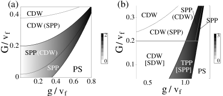
Figure 7: Phase diagrams for a mixture of bosonic and $S=1/2$ fermionic atoms with $v_{b}/v_{f}=5$ and $K_{b}=10$. In (a) $U_{\uparrow\downarrow}/v_{f}=-0.8\pi$ and in (b) $U_{\uparrow\downarrow}/v_{f}=0.8\pi$. Parentheses ($\dots$) indicate subdominant phases.

In Fig. 7 we show two examples for different values of $U_{\uparrow,\downarrow}$. In Fig. 7 (a) we show the phase diagram for $U_{\uparrow,\downarrow}/v_{f}=-0.8\pi$, and in Fig. 7 (b) for $U_{\uparrow,\downarrow}/v_{f}=0.8\pi$. As described above, the system develops a spin gap for $g_{1\perp}<0$. The phase transition occurs at $4\pi G=U_{\uparrow,\downarrow}$. In Fig. 7 b), this corresponds to $G/v_{f}=0.2$, in Fig. 7 (a), the entire phase diagram is in the gapped phase, because $U_{\uparrow,\downarrow}<0$, and $G$ can only be positive.

V.5 Wigner crystal

Apart from these phases the system can also show Wigner crystal (WC) ordering. Within the WC phase, the fermionic atoms crystallize in an alternating pattern of spin-up and spin-down atoms, giving rise to a $4k_{f}$-density modulation. The Wigner crystal order parameter is given by $O_{WC}=\sum_{s}f^{\dagger}_{R,s}f^{\dagger}_{R,-s}f_{L,-s}f_{L,s}\sim\exp[\sqrt{8}i\Theta_{\rho}]$ and has the scaling exponent

$$\alpha_{WC} = 2-4K_{\beta}$$ (78)

Within the gapless phase ($K_{\sigma}=1$), the Wigner crystal phase can become dominant for $K_{\beta}<1/3$, which can be achieved for large values of $G$.

VI Experimental Issues

In this paper we have calculated the phase diagrams of different types of BFMs in various parameter regimes. In this section we will discuss issues concerning the experimental realization of our systems.

Throughout the paper we concentrated on infinite systems at zero temperature, $T=0$. The realization of 1D Luttinger liquids of ultracold atoms will of course be in a finite lattice (around 100 sites) and at finite temperature. At finite temperature the correlation functions become approximately $\langle O(x)O(0)\rangle\sim(\xi\sinh(x/\xi))^{\alpha-2}$, where $\xi\sim v_{f}/k_{B}T$ is the thermal correlation length. For a finite system of length $L=N\lambda_{L}$ ($N$ being the number of lattice sites), the $T=0$-properties of the system are visible for $\xi\sim L$. This corresponds to a temperature regime of $T\sim T_{f}/N$, with $T_{f}$ being the Fermi temperature. So for a system with $N=100$, $T\sim 0.01T_{f}$ is required.

Another issue is the experimental signature of the different phases. Here we present several approaches that can be used to detect the quantum phases discussed above. To detect the CDW phase, one can perform a standard time-of-flight (TOF) measurement. In the CDW phase the fermion density modulation will induce a $2k_{f}$ density wave in the boson field in addition to the zero momentum condensation so that the CDW phase can be observed as interference peaks at momentum $k=2k_{f}$ in a TOF measurement for bosons, whereas the $f$-PP phase will show a featureless superfluid signature. We note that the boundary of an atomic trap and other inhomogeneities in a realistic experiment can pin the CDW phase and generate a true density modulation. One may also use a laser stirring experiment stirring to probe the phase boundary between the insulating (pinned by trap potential) CDW and the superfluid $f$-PP phase: a laser beam is focused at the center of the cloud to create a local potential, and is then moved oscillatory in the condensate. If the system is in the pairing phase, the laser beam can be moved through the system without dissipation, which would manifest itself as heating, if only its velocity is slower than some critical value stirring . At the $f$-PP/CDW phase boundary this critical velocity goes to zero, reflecting a transition to the insulating (CDW) state. This scenario follows from the RG analysis of a single impurity potential kane , as described in Appendix C. To probe the boundary of phase separation one can measure the dipolar collective oscillations of the system, generated by a sudden displacement of the harmonic trap potential with respect to the lattice potential collectivemodes . When the system is near the PS boundary, fermion-boson interaction will reduce the frequency of the dipolar mode essentially to zero, because the two atomic species become immiscible.

As the most promising approach we propose to study the noise correlations of TOF measurements, as discussed in [noise_corr, ]. This type of measurement treats particle-particle correlations (i.e. pairing fluctuations) and particle-hole correlations (i.e. CDW and SDW fluctuations) on equal footing, and therefore reflects the formal duality of these two types of phases accurately. Furthermore, this approach seems to be well-suited for the study of Luttinger liquids, because it gives signatures of the various fluctuations in the system, that dominate in different regimes of the phase diagram.

VII Conclusion

In summary, we used bosonization to investigate the quantum phase diagrams of 1D BFMs. Interactions between atoms can lead to interesting phenomena like spin and charge density waves, singlet and triplet pairing of atoms. We introduced polarons, i.e. atoms of one species surrounded by screening clouds of other species, and argued that the rich phase diagrams of BFMs can be naturally interpreted as Luttinger liquid phase diagrams of such polarons. We also considered several commensurate filling cases and obtained gapped phases in some parameter regimes. We discussed several techniques for probing our results experimentally.

We thank E. Demler, M. Lukin, H. Moritz and B.I. Halperin for useful discussions.

Appendix A Scaling Exponents

In this section we will derive the scaling exponents of a number of operators that were considered in the search for the phase diagram. In section A.1, we discuss BFMs with spinless fermions, and in section A.2 BFMs with spinful fermions.

A.1 Spinless Fermions

For the case of spinless fermions, a broad class of operators $O(x)$ (cp. cazalilla ) can be written in terms of the Luttinger fields as

$$O(x) \sim \exp[\sum_{j=b,f}(i\lambda_{j,1}\Theta_{j}+i\lambda_{j,2}\Phi_{j})]$$ (79)

or a sum of products of this type. $\lambda_{j,1/2}$ are arbitrary real parameters. To derive the correlation function of such an operator we first write $\Theta_{b/f}$ and $\Phi_{b/f}$ in terms of the eigenfields $\Theta_{A/a}$ and $\Phi_{A/a}$, as given by the transformation (35). The correlation function of the above given general operator, $C_{O}(x)=\langle O(x)O(0)\rangle$, then behaves for large distances as :

$$C_{O}(x) \sim |x|^{-\tilde{\alpha}}\cos((\lambda_{f,1}\nu_{f}+\lambda_{b,1}\nu_{b})\pi x),$$ (80)

with the scaling exponent $\tilde{\alpha}$ given by

$$\tilde{\alpha} = \frac{1}{2}(\lambda_{b,1}^{2}K_{\delta}+\lambda_{f,1}^{2}K_{\beta}+2\lambda_{b,1}\lambda_{f,1}K_{\beta\delta}$$ (81)

$$+\lambda_{b,2}^{2}K_{\epsilon}^{-1}+\lambda_{f,2}^{2}K_{\gamma}^{-1}+2\lambda_{b,2}\lambda_{f,2}K_{\gamma\epsilon}^{-1})$$

From this general expression we can deduce the scaling exponents discussed in this paper, by specializing the operator $O(x)$ to various cases.

A.2 Spinful fermions

For the case of spinful fermions, we consider an operator $O(x)$ given by:

$$O(x) \sim \exp[\sum_{j=b,\rho,\sigma}(i\lambda_{j,1}\Theta_{j}+i\lambda_{j,2}\Phi_{j}]$$ (82)

To determine the correlation function of this operator, we proceed as in the previous section. First, we use the linear transformation (67), to write $\theta_{\rho/b}$ in terms of the fields $\theta_{A/a}$. Since the density/boson–sector of the Hamiltonian is just a sum of Gaussian models in terms of these fields, the scaling exponents can be determined as in A.1. For the spin sector we use the RG results discussed in Section V.2: If the non-linear term ir irrelevant the system is described by a Gaussian model with $K_{\sigma}=1$. If the non-linear term is relevant we have $K_{\sigma}\rightarrow 0$, i.e. any overlap of the operator with the phase field $\Phi_{\sigma}$ will make the correlation function short-ranged, whereas the field $\theta_{\sigma}$ acquires ordering.

The correlation function of the operator $O(x)$, $C_{O}(x)=\langle O(x)O(0)\rangle$, can be determined to be:

$$C_{O}(x) = |x|^{-\tilde{\alpha}}\cos((\lambda_{f,1}\nu_{f}+\lambda_{b,1}\nu_{b})\pi x)$$ (83)

The scaling exponent $\tilde{\alpha}$ is given by

$$\tilde{\alpha} = \frac{1}{2}(\lambda_{b,1}^{2}K_{\delta}+\lambda_{\rho,1}^{2}K_{\beta}+2\lambda_{b,1}\lambda_{\rho,1}K_{\beta\delta}$$ (84)

$$+\lambda_{b,2}^{2}K_{\epsilon}^{-1}+\lambda_{\rho,2}^{2}K_{\gamma}^{-1}+2\lambda_{b,2}\lambda_{\rho,2}K_{\gamma\epsilon}^{-1}$$

$$\lambda_{\sigma,1}^{2}K_{\sigma}+\lambda_{\sigma,2}^{2}K^{-1}_{\sigma})$$

In Table 2, we first give the scaling of the single-particle operators $b$ and $f_{{\uparrow}/{\downarrow}}$, as well as the standard order parameters of a LL of spinful fermions, i.e. $f_{s}^{\dagger}f_{s}$ and $f_{\uparrow}^{\dagger}f_{\downarrow}$ (the $2k_{f}$-modes of these operators correspond to CDW and SDW ordering, respectively), the pairing operators $f_{\uparrow}f_{\downarrow}$ (singlet) and $f_{s}f_{s}$ (triplet), and the order parameter of the Wigner crystal, $f^{\dagger}_{\uparrow}f^{\dagger}_{\downarrow}f_{\downarrow}f_{\uparrow}$. Apart from these standard order parameters of LL theory, we consider a wide class of operators of the form $(f_{\uparrow}^{\dagger})^{m}f_{\uparrow}^{n}(f_{\downarrow}^{\dagger})^{p}f_{\downarrow}^{q}(b^{\dagger})^{r}b^{s}$.

Appendix B Polaron Effects

In this subsection we will verify that the conventional construction of polaron operators based on the canonical polaron transformation (CPT) mott is equivalent to the construction within the bosonization approach presented in Section III.1 of this paper. We will also discuss the behavior of the polarization parameter $\lambda_{c}$. The CPT operator is given by

$$U_{\lambda} = e^{-\lambda\sum_{{k}\neq 0}\left(F_{k}\beta_{k}n_{f,k}^{\dagger}-{\rm h.c.}\right)}$$ (85)

where $\beta_{k}$ is the phonon annihilation operator and $n_{f,k}$ is the fermion density operator. $F_{k}$ is given by $F_{k}=\frac{1}{2}\sqrt{\frac{2\pi}{K_{b}|k|L}}$, and $\lambda$ specifies the strength of the phonon dressing.

operator $O(x)$	wavevector $q$	exponent $\tilde{\alpha}$	remarks
$b$	$2mk_{b}$	$\frac{1}{2}\left[(2m)^{2}K_{\delta}+K_{\epsilon}^{-1}\right]$
$f$	$(2n+1)k_{f}$	$\frac{1}{2}[(2n+1)^{2}K_{\beta}+K^{-1}_{\gamma}]$
$f^{\dagger}f$	$2nk_{f}$	$2n^{2}K_{\beta}$	$n\neq 0$
$ff$	$2nk_{f}$	$2n^{2}K_{\beta}+2K^{-1}_{\gamma}$
$b^{\dagger}b$	$2mk_{b}$	$2m^{2}K_{\delta}$	$m\neq 0$
$[b^{\dagger}]^{m_{1}}$	$2mk_{b}$	$\frac{1}{2}\left[(2m)^{2}K_{\delta}+m_{1}^{2}K_{\epsilon}^{-1}\right]$
$[f]^{2n_{1}}$	$2nk_{f}$	$\frac{1}{2}\left[(2n)^{2}K_{\beta}+(2n_{1})^{2}K_{\gamma}^{-1}\right]$
$b^{\dagger}bf^{\dagger}f$	$2mk_{b}+2nk_{f}$	$\frac{1}{2}\left[(2m)^{2}K_{\delta}+(2n)^{2}K_{\beta}-2(2m)(2n)K_{\beta\delta}\right]$	$m,n\neq 0$
$\left[b^{\dagger}\right]^{m_{1}}f^{\dagger}f$	$2mk_{b}+2nk_{f}$	$\frac{1}{2}\left[(2m)^{2}K_{\delta}+(2n)^{2}K_{\beta}-2(2m)(2n)K_{\beta\delta}+m_{1}^{2}K_{\epsilon}^{-1}\right]$	$n\neq 0$
$\left[b^{\dagger}\right]^{m_{1}}\left[f\right]^{2n_{1}}$	$2mk_{b}+2nk_{f}$	$\frac{1}{2}\left[(2m)^{2}K_{\delta}+(2n)^{2}K_{\beta}-2(2m)(2n)K_{\beta\delta}\right.$
		$\ \ \left.+m_{1}^{2}K_{\epsilon}^{-1}+(2n_{1})^{2}K_{\gamma}^{-1}-2m_{1}(2n_{1})K_{\gamma\epsilon}^{-1}\right]$
$\left[b^{\dagger}\right]^{m_{1}}\left[f\right]^{2n_{1}+1}$	$2mk_{b}+(2n+1)k_{f}$	$\frac{1}{2}\left[(2m)^{2}K_{\delta}+(2n+1)^{2}K_{\beta}-2(2m)(2n+1)K_{\beta\delta}\right.$
		$\ \ \left.+m_{1}^{2}K_{\epsilon}^{-1}+(2n_{1}+1)^{2}K_{\gamma}^{-1}-2m_{1}(2n_{1}+1)K_{\gamma\epsilon}^{-1}\right]$
$\tilde{f}$	$(2n+1)k_{f}$	$2-\frac{1}{2}[(2n+1)^{2}K_{\beta}+K^{-1}_{\beta}]$
$\tilde{f}\tilde{f}$	$2nk_{f}$	$2n^{2}K_{\beta}+2K^{-1}_{\beta}$
$\tilde{b}$	$2mk_{b}$	$2-\frac{1}{2}\left[(2m)^{2}K_{\delta}+K_{\delta}^{-1}\right]$

Table 1: Table of Luttinger exponents and characteristic wavevectors of various operators composed of boson and fermion operators. $m$ and $n$ are arbitrary integer number resulting from the higher order harmonics of the bosonization representations.

The sum over the wavevector $k$ is over the regime of acoustic modes. When applied to a fermion operator, the CPT gives

$$U^{-1}_{\lambda}f(x)U_{\lambda} = f(x)e^{-\lambda\sum_{{k}\neq 0}(F_{k}\beta_{k}e^{-i{k}\cdot{r}}-{\rm h.c.})}$$ (86)

which is the standard expression for a fermionic polaron operator mott . In terms of Luttinger bosons the fermion density $n_{f,k}$ is given by:

$$n_{f,k} = \sqrt{{kL}/{2\pi}}(B_{k}+B_{-k}^{\dagger}),$$ (87)

and therefore $U_{\lambda}$ becomes:

$$U_{\lambda} = e^{-\frac{\lambda}{2\sqrt{K_{b}}}\sum_{{k}\neq 0}\left(B_{k}+B_{-k}^{\dagger}\right)\left(\beta_{-k}-\beta_{k}^{\dagger}\right)}$$ (88)

When applied to a fermion operator, this transformation gives

$$U^{-1}_{\lambda}f(x)U_{\lambda} = f(x)e^{-i\lambda\Phi_{b}}$$ (89)

because $U^{-1}_{\lambda}\Phi_{f}U_{\lambda}=\Phi_{f}-\lambda\Phi_{b}$, which can be seen from the operator representation (28) and (30), and by applying the Baker-Hausdorff formula. The superficial difference between Eq. (86) and Eq. (89) can be overcome by a trivial phaseshift $\beta_{k}\rightarrow i{\rm sgn}(k)\beta_{k}$. As discussed in this paper, $\lambda_{c}=K_{\epsilon}/K_{\gamma\epsilon}$ is the most appropiate choice for the fermionic polarons, because the correlation function of such polarons has the slowest algebraic decay.

Figure 8: Plot of the ’dressing’ parameter $\lambda_{c}$ compared to complete dressing $\lambda_{0}$, for $K_{b}=5$ and $G/v_{f}=0.1$ as a function of $g/v_{f}$. With $v_{b}/v_{f}=2,3,5$ for $I$–$III$.

In Fig. 8 we plot this polarization parameter $\lambda_{c}$ in comparison to the value of ’complete dressing’ $\lambda_{0}$:

$$\lambda_{0} = \frac{2g}{v_{b}}\sqrt{K_{b}}$$ (90)

To obtain this quantity, which is the ’size’ the polarization would have if the fermions were static, we set the Fermi velocity to zero ($v_{f}=0$), so that the Hamiltonian of the system becomes:

$$H=\sum_{k\neq 0}v_{b}|k|\beta_{k}^{\dagger}\beta_{k}+\sum_{k\neq 0}g|k|(\beta_{k}^{\dagger}+\beta_{-k})(B_{k}+B_{-k}^{\dagger})$$ (91)

In this limit of infinitely heavy fermions, a term of the type (17) does not exist. In (91) the linear term simply shifts the bosonic modes by an amount $g/v_{b}(B_{k}+B_{-k}^{\dagger})$. As we can see from (88) this corresponds exactly to the polarization $\lambda_{0}$, Eq. (90). However, for finite hopping, or finite mass of the fermions, this value is reduced, because the polarization cloud cannot entirely ’follow’ the fermionic atoms. For $U_{bf}\rightarrow 0$ one finds

$$\lambda_{c}/\lambda_{0} \rightarrow \frac{v_{b}}{v_{b}+v_{f}}$$ (92)

In Fig. 8 we show $\lambda_{c}$ plotted for different sets of parameters. It smoothly interpolates between the small interaction limit (92) and the static limit (90). The static limit is achieved in the vicinity of phase separation because the fermionic effective mode velocity $v_{A}$ goes to zero when the system approaches separation. This corresponds to infinitely heavy fermions, and therefore to the static limit.

operator $O(x)$	wavevector $q$	exponent $\tilde{\alpha}$	remarks
$b$	$2mk_{b}$	$\frac{1}{2}[(2m)^{2}K_{\delta}+K_{\epsilon}^{-1}]$
$f_{{\uparrow}/{\downarrow}}$	$(2n+1)k_{f}$	$(n+\frac{1}{2})^{2}(K_{\beta}+K_{\sigma})+\frac{1}{4}(K_{\gamma}^{-1}+K_{\sigma}^{-1})$
$f^{\dagger}_{s}f_{s}$	$2nk_{f}$	$\left[n^{2}K_{\beta}+n^{2}K_{\sigma}\right]$	$n\neq 0$
$f^{\dagger}_{\uparrow}f_{\downarrow}$	$2(n+m)k_{f}$	$\left[(n+m)^{2}K_{\beta}+(n-m-1)^{2}K_{\sigma}+K_{\sigma}^{-1}\right]$	$n\neq 0$
$f_{s}f_{s}$	$2nk_{f}$	$\left[n^{2}K_{\beta}+n^{2}K_{\sigma}+K^{-1}_{\gamma}+K^{-1}_{\sigma}\right]$
$f_{\uparrow}f_{\downarrow}$	$2(n+l+1)k_{f}$	$\left[(n+l+1)^{2}K_{\beta}+K^{-1}_{\gamma}+(n-l)^{2}K_{\sigma}\right]$
$f_{\uparrow}^{\dagger}f_{\downarrow}^{\dagger}f_{\downarrow}f_{\uparrow}$	$2(n+m)k_{f}$	$\left[(n+m)^{2}K_{\beta}+(n-m)^{2}K_{\sigma}\right]$
$b^{\dagger}b$	$2mk_{b}$	$2m^{2}K_{\delta}$	$m\neq 0$
$[b^{\dagger}]^{m_{1}}$	$2mk_{b}$	$\left[2m^{2}K_{\delta}+\frac{1}{2}m_{1}^{2}K_{\epsilon}^{-1}\right]$
$[f_{s}]^{2n_{1}}$	$2nk_{f}$	$\left[n^{2}(K_{\beta}+K_{\sigma})+n_{1}^{2}(K_{\gamma}^{-1}+K_{\sigma}^{-1})\right]$
$[f_{s}]^{2n_{1}+1}$	$(2n+1)k_{f}$	$\left[(n+\frac{1}{2})^{2}(K_{\beta}+K_{\sigma})+(n_{1}+\frac{1}{2})^{2}(K_{\gamma}^{-1}+K_{\sigma}^{-1})\right]$
$\left[b^{\dagger}\right]^{m_{1}}\left[f_{s}\right]^{2n_{1}}$	$2mk_{b}+2nk_{f}$	$\left[2m^{2}K_{\delta}+n^{2}K_{\beta}-2\sqrt{2}mnK_{\beta\delta}+n^{2}K_{\sigma}\right.$
		$\ \ \left.+\frac{1}{2}m_{1}^{2}K_{\epsilon}^{-1}+n_{1}^{2}K_{\gamma}^{-1}-\sqrt{2}m_{1}n_{1}K_{\gamma\epsilon}^{-1}+n_{1}^{2}K_{\sigma}^{-1}\right]$
$\left[b^{\dagger}\right]^{m_{1}}\left[f\right]^{2n_{1}+1}$	$2mk_{b}+(2n+1)k_{f}$	$\left[2m^{2}K_{\delta}+(n+\frac{1}{2})^{2}K_{\beta}-\sqrt{2}m(2n+1)K_{\beta\delta}+(n+\frac{1}{2})^{2}K_{\sigma}\right.$
		$\ \ \left.+\frac{1}{2}m_{1}^{2}K_{\epsilon}^{-1}+(n_{1}+\frac{1}{2})^{2}K_{\gamma}^{-1}-\sqrt{2}m_{1}(n_{1}+\frac{1}{2})K_{\gamma\epsilon}^{-1}+(n_{1}+\frac{1}{2})^{2}K_{\sigma}^{-1}\right]$
$\left[b^{\dagger}\right]^{m_{1}}\left[f_{\uparrow}f_{\downarrow}\right]$	$2mk_{b}+2(n+l+1)k_{f}$	$\left[2m^{2}K_{\delta}+(n+l+1)^{2}K_{\beta}-2\sqrt{2}m(n+l+1)K_{\beta\delta}+(n-l)^{2}K_{\sigma}\right.$
		$\ \ \left.+\frac{1}{2}m_{1}^{2}K_{\epsilon}^{-1}+K_{\gamma}^{-1}-\sqrt{2}m_{1}K_{\gamma\epsilon}^{-1}\right]$
$\tilde{b}$	$2mk_{b}$	$\frac{1}{2}[(2m)^{2}K_{\delta}+K_{\delta}^{-1}]$
$\tilde{f}_{{\uparrow}/{\downarrow}}$	$(2n+1)k_{f}$	$(n+\frac{1}{2})^{2}(K_{\beta}+K_{\sigma})+\frac{1}{4}(K_{\beta}^{-1}+K_{\sigma}^{-1})$
$\tilde{f}_{s}\tilde{f}_{s}$	$2nk_{f}$	$\left[n^{2}K_{\beta}+n^{2}K_{\sigma}+K^{-1}_{\beta}+K^{-1}_{\sigma}\right]$
$\tilde{f}_{\uparrow}\tilde{f}_{\downarrow}$	$2(n+l+1)k_{f}$	$\left[(n+l+1)^{2}K_{\beta}+K^{-1}_{\beta}+(n-l)^{2}K_{\sigma}\right]$

Table 2: Table of Luttinger exponents and characteristic wavevectors of various order parameters composed by boson and fermion operators for spinful system. $m$, $n$ and $l$ are arbitrary integer number resulting from the higher order harmonics of the bosonization representations.

Appendix C RG flow of an impurity term

We consider the following local impurity term in our Hamiltonian:

$$H_{imp} = \int dxV(x)f^{\dagger}(x)f(x)$$ (93)

with $V(x)$ strongly spatially peaked around at $x=0$. This term leads to an additional term in the action given by

$$S_{imp} = \sum_{m}\frac{v_{m}}{2}\int d\tau\exp(2im\Theta_{f})$$ (94)

where $v_{m}$ is the Fourier transform of the potential $V(x)$ around $2mk_{f}$. The RG flow of these terms at one-loop, as discussed in kane and gnt is given by:

$$\frac{dv_{m}}{dl} = (1-m^{2}K_{\beta})v_{m}$$ (95)

Therefore, such an impurity term is relevant exactly for $K_{\beta}<1$, and irrelevant outside of the CDW phase. The physical interpretation of this result is as follows: In the CDW regime a local impurity ’pins’ the charge ordering of the system. Outside of the CDW phase, the irrelevance of an impurity term in the system is an indication of a superfluid phase, which must be provided by polaron pairing.

References

• (1) D. Jaksch et al., Phys. Rev. Lett. 81, 3108 (1998);
• (2) M. Greiner et al., Nature 415, 39 (2002).
• (3) S.L. Cornish et al., Phys. Rev. Lett. 85, 1795 (2000); S. Inouye et al., Nature 392, 151 (1998).
• (4) G. Modugno, et al., Science 297, 2240 (2002); F. Ferlaino et al., cond-mat/0312255; A. Simoni et al., Phys. Rev. Lett. 90, 163202 (2003).
• (5) Z. Hadzibabic et al., Phys. Rev. Lett. 88, 160401 (2002); G. Roati, et al., Phys. Rev. Lett. 89, 150403 (2002); F. Schreck, et al., Phys. Rev. Lett. 87, 080403 (2001); A.G. Truscott, Science 291, 2570 (2001).
• (6) F. Matera, Phys. Rev A 68, 043624 (2003); D.V. Efremov and L. Viverit, Phys. Rev. B 65, 134519 (2002); L. Viverit, Phys. Rev. A 66, 023605 (2002).
• (7) M.Y. Kagan et. al., cond-mat/0209481; M. Lewenstein et. al., Phys. Rev. Lett. 92, 050401 (2004); H. Fehrmann et. al., cond-mat/0307635.
• (8) R. Roth and K. Burnett, Phys. Rev. A 69, 021601(R) (2004).
• (9) H.P. BΓΌchler and G. Blatter, Phys. Rev. Lett. 91, 130404 (2003).
• (10) For a review of Luttinger liquid in solid state physics, see J. Solyom, Adv. Phys. 28, 201 (1979); J. Voit, Rep. Prog. Phys., 58, 977 (1995).
• (11) S. Tomonaga, Prog. Theor. Phys. 5, 544 (1950).
• (12) J.M. Luttinger, J. Math, Phys. N.Y. 4, 1154 (1963).
• (13) F. D. M. Haldane, J. Phys. C, 14, 2585 (1981).
• (14) F. D. M. Haldane, Phys. Rev. Lett. 47, 1840 (1981).
• (15) L. Mathey, et al., Phys. Rev. Lett. 93, 120404 (2004).
• (16) M.A. Cazalilla, J. Phys. B: AMOP 37, S1-S47 (2004).
• (17) M. A. Cazalilla and A. F. Ho, Phys. Rev. Lett. 91, 150403 (2003).
• (18) A. Gorlitz et al., PRL 87, 130402 (2001); S. Dettmer et al., PRL 87, 160406 (2001).
• (19) W. Hansel, et. al., Nature 413 498 (2001); J.H. Thywissen, et. al., Eur. Phys. J. D. 7, 361 (1999); R. Folman, et. al., Adv. At. Mol. Opt. Phys. 48, 263 (2002).
• (20) S. Foelling et al., Nature 434, 481 (2005);
• (21) C.J. Pethick and H. Smith, Bose-Einstein Condensation in Dilute Gases (Cambridge University Press, 2004).
• (22) H. Moritz, private communication
• (23) A.P. Albus, et al., Phys. Rev. A 67, 063606 (2003); M.J. Bijlsma, et al., Phys. Rev. A 61, 053601 (2000).
• (24) M. Kramer, et. al., Phys. Rev. Lett. 88, 180404 (2002).
• (25) J. Voit and Schulz, Phys. Rev. B 36, 968 (1987); ibid 37, 10068 (1988).
• (26) S. Engelsberg and B.B. Varga , Phys. Rev. 136, A1582 (1964).
• (27) A. De Martino and R. Egger, Phys. Rev. B 235418 (2003).
• (28) T. Martin, and D. Loss, Int. J. Mod. Phys. 9, 495 (1995).
• (29) V. Meden et. al., Phys. Rev. B 50, 11179 (1994).
• (30) R. Sankar, Acta Phys. Pol. B 26, 1835 (1995).
• (31) A.S. Alexandrov and S.N. Mott, Polarons and Bipolarons (World Scientific, Singapore, 1995).
• (32) L. Mathey, cond-mat/0602616.
• (33) A.O. Gogolin, A.A. Nerseyan and A.M. Tsvelik, Bosonization and Strongly Correlated Systems (Cambridge University Press, 1998).
• (34) C. Raman, et. al., Phys. Rev. Lett. 83, 2502 (1999); R. Onofrio, et. al., Phys. Rev. Lett. 85, 2228 (1999).
• (35) L. Mathey, et al., cond-mat/0507108.
• (36) P. Maddaloni, et al., Phys. Rev. Lett. 85, 2413 (2000); S.D. Gensemer and D.S. Jin, Phys. Rev. Lett. 87, 173201 (2001); L. Vichi et al., Phys. Rev. A 60, 4734 (1999).
• (37) C. Kane and M.P.A. Fisher, Phys. Rev. Lett. 68, 1220 (1992).
• (38) N. N. Bogoliubov, J. Phys. (U.S.S.R.) 11, 23 (1947).
• (39) C. Mora and Y. Castin, Phys. Rev. A 67, 053615 (2003).