Dynamics of Random Packings in Granular Flow

Abstract

We present a multiscale simulation algorithm for amorphous materials, which we illustrate and validate in a canonical case of dense granular flow. Our algorithm is based on the recently proposed Spot Model, where particles in a dense random packing undergo chain-like collective displacements in response to diffusing “spots” of influence, carrying a slight excess of interstitial free volume. We reconstruct the microscopic dynamics of particles from the “coarse grained” dynamics of spots by introducing a localized particle relaxation step after each spot-induced block displacement, simply to enforce packing constraints with a (fairly arbitrary) soft-core repulsion. To test the model, we study to what extent it can describe the dynamics of up to 135,000 frictional, viscoelastic spheres in granular drainage simulated by the discrete-element method (DEM). With only five fitting parameters (the radius, volume, diffusivity, drift velocity, and injection rate of spots), we find that the spot simulations are able to largely reproduce not only the mean flow and diffusion, but also some subtle statistics of the flowing packings, such as spatial velocity correlations and many-body structural correlations. The spot simulations run over 100 times faster than DEM and demonstrate the possibility of multiscale modeling for amorphous materials, whenever a suitable model can be devised for the coarse-grained spot dynamics.

I Introduction

The geometry of static sphere packings is an age-old problem Torquato (2003) with current work focusing on jammed random packings Torquato et al. (2000); O’Hern et al. (2003), but how do random packings flow? Here, we consider the case of granular drainage Jaeger et al. (1996), which is of practical importance (e.g. in pebble-bed nuclear reactors Talbot (2002); Rycroft et al. ) and also raises fundamental questions in non-equilibrium statistical mechanics Kadanoff (1999). In fast, dilute flows, Boltzmann’s kinetic theory of gases can be modified to account for inelastic collisions Jenkins and Savage (1983), but slow, dense flows (as in Fig. 1) require a different description due to long-lasting, many-body contacts Choi et al. (2004). Although ballistic motion may occur at the nano-scale Menon and Durian (1997) ($<0.01$% of a grain diameter), collisions do not result in random recoils, as in a gas.

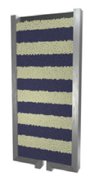
(a) (b)

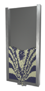
Figure 1: (Color online) A simulation of the experiment in Ref. Choi et al. (2004) by discrete element simulations. (a) First, 55,000 glass beads are poured into a quasi-two-dimensional silo (8 beads deep) and let come to rest. (b) Slow drainage occurs after a slit orifice is opened. (The grains are identical, but colored by their initial height.)

In crystals, diffusion and flow are mediated by defects, such as vacancies and dislocations, but in disordered phases it is not clear what, if any, “defects” might facilitate structural rearrangements. Perhaps the only candidate in the literature is an empty “void” in the random packing into which a single particle may hop, thereby displacing the void. The void mechanism was proposed by Eyring for viscous flow Eyring (1936) and has re-appeared in theories of the glass transition Cohen and Turnbull (1959), shear flow in metallic glasses Spaepen (1977), compaction in vibrated granular materials Boutreux and de Gennes (1997), and granular drainage from a silo Mullins (1972), but it is now seen as unrealistic. In glasses, cooperative relaxation (involving many particles at once) has been observed Donati et al. (1998); Weeks et al. (2000), presumably facilitated by free volume Cohen and Grest (1979); Lemaître (2002); Garrahan and Chandler (2003). In granular drainage, the Void Model gives a reasonable fit to the mean flow Tüzün and Nedderman (1979); Choi et al. (2005), and yet it grossly over-predicts diffusion Choi et al. (2004).

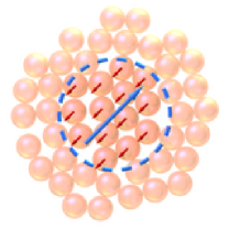
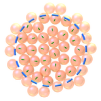
(a) (b) (c)

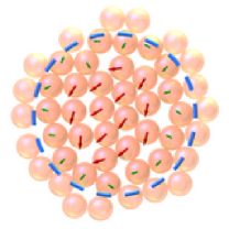
Figure 2: (Color online) The mechanism for structural rearrangement in the Spot Model. The random displacement $\mathbf{r}_{s}$ of a diffusing spot of free volume (dashed circle) causes affected particles to move as a block by an amount $\mathbf{r}_{p}$ (a), followed by an internal relaxation with soft-core repulsion (b), which yields the net cooperative motion (c). (The displacements, typically 100 times smaller than the grain diameter, are exaggerated for clarity.)

A collective mechanism for random-packing dynamics has recently been proposed to resolve this paradox and applied to granular drainage Bazant (2005). The basic hypothesis, shown in Fig. 2(a), is that a block of neighboring grains makes a small, correlated downward displacement,

$$\Delta\mathbf{r}_{p}=-w\Delta\mathbf{r}_{s},$$ (1)

in response to the random upward displacement, $\Delta\mathbf{r}_{s}$, of a diffusing “spot” of free volume. The coefficient $w$ (more generally, a smooth function of the particle-spot separation) is set by local volume conservation. In the simplest approximation, a spot carries a slight excess of interstitial volume, $V_{s}$, spread uniformly across a sphere of radius $R_{s}$. When the spot engulfs $N$ particles, each of volume $V_{p}$, the model predicts $w\approx V_{s}/NV_{p}\approx\Delta\phi/\phi^{2}$, where $\Delta\phi$ is the local change in volume fraction $\phi$. Allowing for some spot overlaps yields the estimate $w\approx 10^{-2}-10^{-3}$ from the observation that $\Delta\phi/\phi\approx 1\%$ in dense flows, which is consistent with diffusion measurements in experiments Choi et al. (2004, 2005) and our simulations below. Unlike the Void Model (which requires $w=1$), each grain’s “cage” of nearest neighbors also persists over long distances Choi et al. (2004); the Spot Model is able to capture such features of drainage experiments, while remaining simple enough for mathematical analysis, because it does not explicitly enforce packing constraints, only the tendency of nearby particles to diffuse together.

In order to preserve valid packings, a multiscale spot algorithm has also been suggested Bazant (2005), which we implement here for the first time. As shown in Fig. 2, each spot-induced block displacement (a) is followed by a relaxation step (b), in which the affected particles and their nearest neighbors experience a soft-core repulsion (with all other particles held fixed). The net displacement in (c) involves a cooperative local deformation, whose mean is roughly the block motion in (a). It is not clear a priori that this procedure can produce realistic flowing packings, and, if so, whether the relaxation step dominates the simple dynamics from the original model.

To answer these questions, we calibrate and test the Spot Model against large-scale computer simulations of granular drainage, shown in Fig. 1. Simulations are advantageous in this case since three-dimensional packing dynamics cannot easily be observed experimentally. We begin by running discrete-element method (DEM) simulations, described in section II. We then calibrate the free parameters in the Spot Model by measuring various statistical quantities from the DEM simulation, as described in III. In section IV, we describe the computational implementation of the Spot Model, before carrying out a detailed comparison to DEM in section V.

II DEM Simulation method

We employ a DEM Cundall and Strack (1979); Landry et al. (2003) to simulate $N$ frictional, visco-elastic, spherical glass beads of diameter, $d=3\textrm{mm}$, mass $m$ under the influence of gravity $g=9.81\textrm{ms}^{-1}$. Similar to the experiments of Refs. Choi et al. (2004, 2005) the silo has width $50d$ and thickness $8d$ with side walls at $x=\pm 25d$ and front and back walls at $y=\pm 4d$, all with friction coefficient $\mu=0.5$. The initial packing is generated by pouring $N=55,000$ particles in from a fixed height of $z=170d$ and allowing them to come to rest under gravity, filling the silo up to $H_{o}\approx 110d$. We also studied a taller system with $N=135,000$ generated by pouring particles in from a height of $z=495d$, which fills the silo to $H_{o}\approx 230d$. We refer to these systems by their initial height $H_{o}$. Drainage is initiated by opening a circular orifice of width $8d$ centered at $x=y=0$ in the base of the silo ($z=0$). A snapshot of all particle positions is recorded every $2\times 10^{4}$ time steps ($\delta t=1.75\times 10^{-6}\textrm{s}$). Once particles drop below $z=-10d$, they are removed from the simulation.

The particles interact according to Hertzian, history dependent contact forces. If a particle and its neighbor are separated by a distance $\mathbf{r}$, and they in compression, so that $\delta=d-\left|\mathbf{r}\right|>0$, then they experience a force $\mathbf{F}=\mathbf{F}_{n}+\mathbf{F}_{t}$, where the normal and tangential components are given by

$$\mathbf{F}_{n} = \sqrt{\delta/d}\left(k_{n}\delta\mathbf{n}-\frac{\gamma_{n}\mathbf{v}_{n}}{2}\right)$$ (2)

$$\mathbf{F}_{t} = \sqrt{\delta/d}\left(-k_{t}\Delta\mathbf{s}_{t}-\frac{\gamma_{t}\mathbf{v}_{t}}{2}\right).$$ (3)

Here, $\mathbf{n}=\mathbf{r}/\left|\mathbf{r}\right|$. $\mathbf{v}_{n}$ and $\mathbf{v}_{t}$ are the normal and tangential components of the relative surface velocity, and $k_{n,t}$ and $\gamma_{n,t}$ are the elastic and viscoelastic constants, respectively. $\Delta\mathbf{s}_{t}$ is the elastic tangential displacement between spheres, obtained by integrating tangential relative velocities during elastic deformation for the lifetime of the contact, and is truncated as necessary to satisfy a local Coulomb yield criterion $\left|\mathbf{F}_{t}\right|\leq\mu\left|\mathbf{F}_{n}\right|$. Particle-wall interactions are treated identically, but the particle-wall friction coefficient is set independently. For the current simulations we set $k_{t}=\frac{2}{7}k_{n}$, and choose $k_{n}=2\times 10^{5}mg/d$. While this is significantly less than would be realistic for glass spheres, where we expect $k_{n}\sim 10^{10}mg/d$, such a spring constant would be prohibitively computationally expensive, as the time step must have the form $\delta t\propto k_{n}^{-1/2}$ for collisions to be modeled effectively. Previous simulations have shown that increasing $k_{n}$ does not significantly alter physical results Landry et al. (2003). We make use of a time step of $\delta t=1.75\times 10^{-6}\textrm{s}$, and damping coefficients $\gamma_{n}=\gamma_{t}=50\sqrt{g/d}$.

III Calibration of the model

We first look for evidence of spots in the DEM simulation and then proceed to calibrate the model. All the calibrations are carried out for the small $H_{o}=110d$ system, after which the same parameters are used for the larger $H_{o}=230d$ system.

The theory predicts large numbers of spots (since many are released as each particle exits the silo), so we seek a statistical signature of the passage of many spots. We therefore consider the spatial correlation for velocities in the $x$ direction, defined by

$$C(r)=\frac{\left\langle u_{x}(0)u_{x}(r)\right\rangle}{\sqrt{\left\langle u_{x}(0)^{2}\right\rangle\left\langle u_{x}(r)^{2}\right\rangle}}$$

where the expectations are taken over all pairs of velocities $(u_{x}(0),u_{x}(r))$ of particles separated by a distance $r$ in a given test region. For a uniform spot influence out to a cutoff radius, $R_{s}>d$, as shown in Fig. 2(a), two random particle displacements are either identical, if they are caused by the same spot, or independent. In that case, the spatial velocity correlation function is given by

$$C(r)=\left\{\begin{array}[]{ll}1-\frac{3}{4}\frac{r}{R_{s}}+\frac{1}{16}\left(\frac{r}{R_{s}}\right)^{3}&r<2R_{s}\\ 0&r\geq 2R_{s}\\ \end{array}\right.$$ (4)

which is the intersection volume of spheres of radius $R_{s}$ separated by $r$ (scaled to $1$ at $r=0$). The shape of $C(r)$ is affected by the relaxation step in Fig. 2(b), but the decay length is set by the spot size.

Figure 3: (Color online) Comparison of velocity correlations calculated over the time period $0.52\textrm{s}<t<1.57\textrm{s}$. Calculations are based on particle velocity fluctuations about the mean flow in a $16d\times 16d$ region high in the center of the container. For $H_{o}=110d$.

As shown in Fig. 3, we see spatial velocity correlations in the DEM simulations at the scale of several particle diameters, consistent with the spot hypothesis. Similar correlations have also been seen in experiments Choi using the methods of Choi et al. Choi et al. (2004), which attests to the generality of the phenomenon, as well as the realism of the simulations. Since the shape of $C(r)$ is not precisely that of Eq. (4), due to relaxation effects, we fit the simulation data to a simple decay, $C(r)=\alpha e^{-r/\beta}$ with $\beta=1.87d$. We also fit a simple decay of the same form to Eq. (4), finding $\beta=0.72R_{s}$, so we infer $R_{s}=2.60d$ as the spot radius. Thus a grain has significant dynamical correlations with neighbors up to three diameters away.

Next, we infer the dynamics of spots, postulating independent random walks as a first approximation. We assume that spots drift upward at a constant mean speed, $v_{s}=\Delta z_{s}/\Delta t$, (determined below), opposite to gravity, while undergoing random horizontal displacements of size $\Delta x_{s}$ in each time step $\Delta t$. The spot diffusion length, $b_{s}=\operatorname{Var}(\Delta x_{s})/2\Delta z_{s}$, is obtained from the spreading of the mean flow away from the orifice. In DEM simulations, the horizontal profile of the vertical velocity component is well described by a Gaussian, whose variance grows linearly with height, as shown in Fig. 4. Applying linear regression gives $\operatorname{Var}(u_{z})=2.28zd+1.60d^{2}$, which implies $b_{s}=2.28d/2=1.14d$. To reproduce the spot diffusion length, we chose $\Delta z_{s}=0.1d$ and $\Delta x_{s}=0.68d$.

Figure 4: (Color online) Comparison of the mean velocity profile, for three different heights calculated over the time period $4.37\textrm{s}<t<5.25\textrm{s}$ once steady flow has been established. The Spot Model successfully predicts a Gaussian velocity profile near the orifice and the initial spreading of the flow region with increasing height, although the DEM flow becomes more plug-like higher in the silo.

The typical excess volume carried by a spot can now be obtained from a single bulk diffusion measurement. From Eq. (1), the particle diffusion length, $b_{p}$, is given by

$$b_{p}=\frac{\operatorname{Var}(\Delta x_{p})}{2\Delta z_{p}}=\frac{\operatorname{Var}(w\Delta x_{s})}{2w\Delta z_{s}}=wb_{s}.$$

We measure $b_{p}$ in the DEM simulation by tracking the variance of the $x$ displacements of particles that start high in the silo as a function of their distance dropped. We find $b_{p}=2.86\times 10^{-3}d$ and thus $w=2.50\times 10^{-3}$. During steady flow in the DEM simulation, a typical packing fraction of particles is $57.9\%$, so a spot with radius $R_{s}=2.60d$ influences on average $81.7$ other particles. Thus we find that a spot carries roughly $20\%$ of a particle volume: $V_{s}=81.7V_{p}/w=0.205V_{p}$.

The three spot parameters so far (radius, $R_{s}$, diffusion length, $b_{s}$, and influence factor, $w$) suffice to determine the geometrical features of a steady flow, such as the spatial distribution of mean velocity and diffusion, but two more are needed to introduce time dependence. The first is the mean rate of creating spots at the orifice (for simplicity, according to a Poisson process). In the DEM simulation, particles exit a rate of mean rate of $4.40\times 10^{3}\textrm{s}^{-1}$, so spots carrying a typical volume $V_{s}=0.205V_{p}$ should be introduced at a mean rate of $\nu_{s}=2.15\times 10^{4}\textrm{s}^{-1}$. The second remaining spot parameter is the vertical drift speed, or, equivalently, the mean waiting time between spot displacements, $\Delta t$, which can be inferred from the drop in mean packing fraction during flow. In the DEM simulation, we find that there are initially $9,400$ particles in the horizontal slice, $50d<z<70d$, which drops to $8,850$ during flow. Choosing the spot waiting time to be $\Delta t=8.68\times 10^{-4}$s reproduces this decrease in density in the spot simulation. The spot drift speed is thus $v_{s}=0.1d/\Delta t=115d/\textrm{s}=34.5\textrm{cm}/\textrm{s}$, which is roughly ten times faster than typical particle speeds in Fig. 4.

IV Spot model simulation

Having calibrated the five parameters ($R_{s}$, $b_{s}$, $w$, $\nu_{s}$, $v_{s}$), we can test the Spot Model by carrying out drainage simulations starting from the same static initial packing as for the DEM simulations. For efficiency, a standard cell method (also used in the parallel DEM code) is adapted for the spot simulations. The container is partitioned into a grid of $10\times 3\times N_{z}$ cells, each responsible for keeping track of the particles within it, with $N_{z}=30$ for $H_{o}=110d$ and $N_{z}=60$ for $H_{o}=230d$. When a spot moves, only the cells influenced by the spot need to be tested, and particles are transferred between cells when necessary. Without further optimization, the multiscale spot simulation runs over 100 times faster than the DEM simulation.

The flow is initiated as spots are introduced uniformly at random positions on the orifice (at least $R_{s}$ away from the edges) at random times according to a Poisson process of rate $\nu_{s}$. (The waiting time is thus an exponential random variable of mean $\nu_{s}^{-1}$.) Once in the container, spots also move at random times with a mean waiting time, $\Delta t=v_{s}/\Delta z_{s}$. Spot displacements in the bulk are chosen randomly from four displacement vectors, $\Delta\mathbf{r}_{s}=(\pm\Delta x_{s},0,\Delta z_{s}),(0,\pm\Delta x_{s},\Delta z_{s})$, with equal probability, so spots perform directed random walks on a body-centered cubic lattice (with lattice parameter $2\Delta z_{s}=0.2d$). We make this simple choice to accelerate the simulation because more complicated, continuously distributed and/or smaller spot displacements with the same drift and diffusivity give very similar results. Spot centers are constrained not to come within $d$ of a boundary, and once a spot reaches the top of the packing, it is removed from the simulation. More realistic models for the orifice, walls, and free surface are left for future work; here we focus on flowing packings in the bulk.

Discrete Element Method

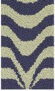
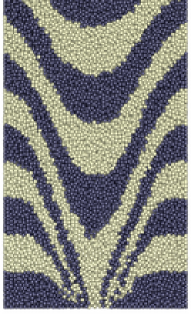
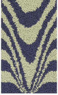
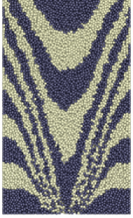
Spot Model

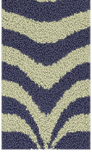
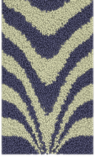
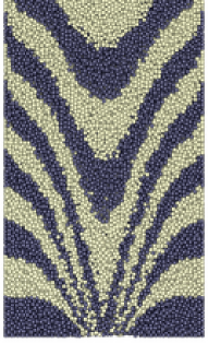
$t=1.05$s                          $t=2.10$s                          $t=3.15$s                          $t=4.20s$

Figure 5: (Color online) Time evolution of the random packing (from left to right) in DEM (top) and the spot simulation (bottom), for the $H_{o}=230d$ system, starting from the same initial state. Each image is a vertical slice through the center of the silo near the orifice well below the free surface.

The particles in the simulation move passively in response to spot displacements without any lattice constraints. Although the influence of a spot can take a very general form Bazant (2005), the most important aspect is its length scale, so here we choose the simplest possible model in Eq. (1), where the spot influences particles uniformly in a sphere of radius $R_{s}$. As shown in Fig. 2(a), we center the spot influence on the midpoint of its step, which seems the most consistent with the concept of moving interstitial volume from the initial to the final spot position. To be precise, when a spot moves from $\mathbf{r}_{s}$ to $\mathbf{r}_{s}+\Delta\mathbf{r}_{s}$, all particles less than $R_{s}$ away from $\mathbf{r}_{s}+\Delta\mathbf{r}_{s}/2$ are displaced by $-w\Delta\mathbf{r}_{s}$.

To preserve realistic packings, we carry out a simple elastic relaxation after each spot-induced block motion, as in Fig. 2(b). All particles within a radius $R_{s}+2d$ of the midpoint of the spot displacement exert a soft-core repulsion on each other, if they begin to overlap. Rather than relaxing to equilibrium or integrating Newton’s laws, however, we use the simplest possible algorithm: Each pair of particles separated by less than $d$ moves apart with identical and opposite displacements, $(d-r)\alpha$, for some constant $\alpha>1$. Similarly, a particle within $d/2$ of a wall moves away by a displacement, $(\frac{d}{2}-r)\alpha$. Particle positions are updated simultaneously once all pairings are considered, but those within the shell, $R_{s}+d<r<R_{s}+2d$, more than one diameter away from the initial block motion, are held fixed to prevent long-range disruptions.

It turns out that, due to the cooperative nature of Spot Model, only extremely small relaxation is required to enforce packing constraints, mainly near spot edges where some shear occurs. Here, we choose $\alpha=0.8$ and find that the displacements due to relaxation are typically less than 25% of the initial block displacement, which is at the scale of 1/10,000 of a particle diameter: $0.25w\Delta r_{s}\approx 2\times 10^{-4}d$. Due to this tiny scale, the details of the relaxation do not seem to be very important; we have obtained almost indistinguishable results with $\alpha=0.6$ and $\alpha=1.0$ and also with more complicated energy minimization schemes. As such, we do not view the soft-core repulsion as introducing any new parameters.

V Results

The spot and DEM simulations are compared using snapshots of all particle positions taken every $2\times 10^{4}$ time steps. As shown in Figure 5, the agreement between the two simulations is remarkably good, considering the small number of parameters and physical assumptions in the Spot Model. It is clear a posteriori that the relaxation step, in spite of causing only minuscule extra displacements, manages to produce reasonable packings during flow, while preserving the realistic description of the mean velocity and diffusion in the basic Spot Model. Only one parameter, $b_{s}$, is fitted to the mean flow, but we find that the entire velocity profile is accurately reproduced in the lower part of the container, as shown in Fig. 4, although the flow becomes somewhat more plug-like in DEM simulation higher in the container. Similarly, we fit $w$ to the particle diffusion length in middle of the DEM simulation, $b_{p}=2.86\times 10^{-3}d$, without accounting for the elastic relaxation step, so it is reassuring that the same measurement in the spot simulation yields a similar value, $b_{p}=2.73\times 10^{-3}d$.

The most surprising findings concern the agreement between the DEM and spot simulations for various microscopic statistical quantities. First, we consider the radial distribution function, $g(r)$, which is the distribution of inter-particle separations, scaled to the same quantity in a ideal gas at the same density. For dense sphere packings, the distribution begins with a large peak near $r=d$ for particles in contact and smoothly connects smaller peaks at typical separations of more distant neighbors, while decaying to unity. As shown in Fig. 6(a), the functions $g(r)$ from the spot and DEM simulations are nearly indistinguishable, across the entire range of neighbors for the $H_{o}=110d$ system. This cannot be attributed entirely to the initial packing because each simulation evolves independently through substantial drainage and shearing.

Next, we consider the three-body correlation function, $g_{3}(\theta)$, which gives the probability distribution for “bond angles” subtended by separation vectors to first neighbors (defined by separations less than the first minimum of $g(r)$ at $1.38d$). For sphere packings, $g_{3}(\theta)$ has a sharp peak at $60^{\circ}$ for close-packed triangles, and another broad peak around $110-120^{\circ}$ for larger crystal-like configurations. In Fig. 6(b), we reach the same conclusion for $g_{3}(\theta)$ as for $g(r)$: The spot and DEM simulations evolve independently from the initial packing to nearly indistinguishable steady states.

Figure 6: (Color online) Comparison of radial distribution functions (top) and bond angles (bottom) for particles in the region $-15d<x<15d$, $15d<z<45d$ for $H_{o}=110d$ system. Three curves are shown on each graph, the first calculated from the initial static packing (common between the two simulations), and the second and third calculated for over the range $1.04\textrm{s}<t<1.40\textrm{s}$.

The striking agreement between the spot and DEM simulations seems to apply not only to structural, but also to dynamical, statistical quantities. Returning to Fig. 3, we see that the two simulations have very similar spatial velocity correlations. Of course, the spot size, $R_{s}$, in the Spot Model (without relaxation) was fitted roughly to the scale of the correlations in the DEM simulation, but the multiscale spot simulation also manages to reproduce most of the fine structure of the correlation function.

At much longer times, however, the random packings are no longer indistinguishable, as a small tendency for local close-packed ordering appears the spot simulation. As shown in Fig. 7, the spot simulation develops enhanced crystal-like peaks in $g(r)$ at $r=\sqrt{3}d$, $2d$, $\ldots$. The number of particles involved, however, is very small ($\sim 2\%$), and the effect seems to saturate, with no significant change between $8\textrm{s}$ and $16\textrm{s}$. This is consistent with even longer spot simulations in systems with periodic boundary conditions, which reach a similar, reproducible steady state (at the same volume fraction) from a variety of initial conditions Palacci (2005). In all cases, the spot algorithm never breaks down (e.g. due to jamming or instability), and unrealistic packings with overlapping particles are never created.

The structure of the flowing steady state is fairly insensitive to various details of the spot algorithm. For example, changing the relaxation parameter (in the range $0.6\leq\alpha\leq 1.0$), rescaling the spot size (by $\pm 25\%$), and using a persistent random walk (for smoother spot trajectories), all have no appreciable effect on $g(r)$. On the other hand, decreasing the vertical spot step size (in the range $0.025d\leq\Delta z\leq 0.1d$) tends to inhibit spurious local ordering and reduce the difference in $g(r)$ between the spot and DEM simulations (e.g. measured by the $L_{2}$ norm). Therefore, our spot algorithm appears to “converge” with decreasing time step (and increasing computational cost), analogous to a finite-difference method, although this merits further study.

Figure 7: (Color online) Evolution of the radial distribution function $g(r)$ for $H_{o}=230d$ in the region $-15d<x<15d$, $15d<z<45d$. The spot simulation (dashed curves) reaches a somewhat different steady state from the DEM simulation (solid curve), after a large amount of drainage has taken place.

VI Conclusions

Our results suggest that flowing dense random packings have some universal geometrical features. This would be in contrast to static dense random packings, which suffer from ambiguities related to the degree of randomness and definitions of jamming Torquato et al. (2000); O’Hern et al. (2003). The similar packing dynamics in spot and DEM simulations suggest that geometrical constraints dominate over mechanical forces in determining structural rearrangements, at least in granular drainage. Some form of the Spot Model may also apply to other granular flows and perhaps even to glassy relaxation, where localized, cooperative motion also occurs Donati et al. (1998); Weeks et al. (2000).

The Spot Model provides a simple framework for the multiscale modeling of liquids and glasses, analogous to dislocation dynamics in crystals. Our algorithm, which combines an efficient, “coarse-grained” simulation of spots with limited, local relaxation of particles, runs over 100 times faster than fully particle-based DEM for granular drainage. On current computers, this means that simulating one cycle of pebble-bed reactor Talbot (2002) can take hours instead of weeks Rycroft et al. , although a general theory of spot motion in different geometries is still lacking. This may come from a stochastic formulation of Mohr-Coulomb plasticity, where spots perform random walks along slip lines of incipient failure Kamrin and Bazant , which could, in principle, be applied to different materials by changing the yield criterion. Alternatively, a multiscale model for supercooled molecular liquids could involve spots moving along chains of dynamic facilitation Garrahan and Chandler (2003); Jung et al. (2004). In any case, we have demonstrated that dense random-packing dynamics can be driven entirely by the motion of simple, collective excitations.

References

- Torquato (2003) S. Torquato, Random Heterogeneous Materials (Springer, New York, 2003).
- Torquato et al. (2000) S. Torquato, T. M. Truskett, and P. G. Debenedetti, Phys. Rev. Lett. 84, 2064 (2000).
- O’Hern et al. (2003) C. S. O’Hern, L. E. Silbert, A. J. Liu, and S. R. Nagel, Phys. Rev. E 68, 011306 (2003).
- Jaeger et al. (1996) H. M. Jaeger, S. R. Nagel, and R. P. Behringer, Rev. Mod. Phys. 68, 1259 (1996).
- Talbot (2002) D. Talbot, MIT Technology Review pp. 54–59 (2002).
- (6) C. H. Rycroft, G. S. Grest, J. W. Landry, and M. Z. Bazant, (unpublished) .
- Kadanoff (1999) L. P. Kadanoff, Rev. Mod. Phys. 71, 435 (1999).
- Jenkins and Savage (1983) J. T. Jenkins and S. B. Savage, J. Fluid Mech. 130, 187 (1983).
- Choi et al. (2004) J. Choi, A. Kudrolli, R. R. Rosales, and M. Z. Bazant, Phys. Rev. Lett. 92, 174301 (2004).
- Menon and Durian (1997) M. Menon and D. J. Durian, Science 275, 1920 (1997).
- Eyring (1936) H. Eyring, J. Chem. Phys. 4, 283 (1936).
- Cohen and Turnbull (1959) M. H. Cohen and D. Turnbull, J. Chem. Phys. 31, 1164 (1959).
- Spaepen (1977) F. Spaepen, Acta Metallurgica 25, 407 (1977).
- Boutreux and de Gennes (1997) T. Boutreux and P. G. de Gennes, Physica A 244, 59 (1997).
- Mullins (1972) J. Mullins, J. Appl. Phys. 43, 665 (1972).
- Donati et al. (1998) C. Donati, J. F. Douglas, W. Kob, S. J. Plimpton, P. H. Poole, and S. C. Glotzer, Phys. Rev. Lett. 80, 2338 (1998).
- Weeks et al. (2000) E. R. Weeks, J. C. Crocker, A. C. Levitt, A. Schofield, and D. A. Weitz, Science 287, 627 (2000).
- Cohen and Grest (1979) M. C. Cohen and G. S. Grest, Phys. Rev. B 20, 1077 (1979).
- Lemaître (2002) A. Lemaître, Phys. Rev. Lett. 89, 195503 (2002).
- Garrahan and Chandler (2003) J. P. Garrahan and D. Chandler, Proc. Nat. Acad. Sci. 100, 9710 (2003).
- Tüzün and Nedderman (1979) U. Tüzün and R. M. Nedderman, Powder Technolgy 23, 257 (1979).
- Choi et al. (2005) J. Choi, A. Kudrolli, and M. Z. Bazant, J. Phys.: Condensed Matter 17, S2533 (2005).
- Bazant (2005) M. Z. Bazant, Mechanics of Materials (2005), (to appear).
- Cundall and Strack (1979) P. A. Cundall and O. D. L. Strack, Geotechnique 29, 47 (1979).
- Landry et al. (2003) J. W. Landry, G. S. Grest, L. E. Silbert, and S. J. Plimpton, Phys. Rev. E 67, 041303 (2003).
- (26) J. Choi, private communication.
- Palacci (2005) J. Palacci, Tech. Rep., MIT Department of Mathematics (2005).
- (28) K. Kamrin and M. Z. Bazant, (unpublished) .
- Jung et al. (2004) Y. Jung, J. P. Garrahan, and D. Chandler, Phys. Rev. E 69, 061205 (2004).