Extended quasimodes within nominally localized random waveguides

Abstract

We have measured the spatial and spectral dependence of the microwave field inside an open absorbing waveguide filled with randomly juxtaposed dielectric slabs in the spectral region in which the average level spacing exceeds the typical level width. Whenever lines overlap in the spectrum, the field exhibits multiple peaks within the sample. Only then is substantial energy found beyond the first half of the sample. When the spectrum throughout the sample is decomposed into a sum of Lorentzian lines plus a broad background, their central frequencies and widths are found to be essentially independent of position. Thus, this decomposition provides the electromagnetic quasimodes underlying the extended field in nominally localized samples. When the quasimodes overlap spectrally, they exhibit multiple peaks in space.

The nature of wave propagation in disordered samples reflects the spatial extent of the wave within the medium. Anderson ; Thouless ; gangof4 In part because of the inaccessibility of the interior of multiply-scattering samples, the problem of transport in the presence of disorder has been treated as a scattering problem with the transition from extended to localized waves charted in terms of characteristics of conductance and transmission. When gain, loss, and dephasing are absent, the nature of transport can be characterized by the degree of level overlap, $\delta$, Thouless ; gangof4 which is the ratio of average width and spacing of states of an open random medium, $\delta\equiv\delta\nu/\Delta\nu$. Here $\delta\nu$ may be identified with the spectral width of the field correlation function Genack and $\Delta\nu$ with the inverse of the density of states of the sample. When $\delta>1$, resonances of the sample overlap spectrally, the wave spreads throughout the sample and transport is diffusive. Thouless In contrast, when $\delta<1$, coupling of the wave in different portions of the sample is impeded. Azbel showed that,when $\delta<1$, transmission may occur via resonant coupling to exponentially peaked localized modes with spectrally isolated Lorentzian lines with transmission approaching unity when the wave is localized near the center of the sample. Azbel ; Freilikher Given the sharp divide postulated between extended and localized waves, the nature of propagation when modes occasionally overlap in samples for which $\delta<1$ is of particular interest.

Mott argued that interactions between closely clustered levels in a range of energy in which $\delta<1$ would be associated with two or more centers of localization within the sample within the sample. Mott Pendry showed that, in this case, occasionally overlapping of electronic modes play an outsized role in transport since electrons may then flow through the sample via regions of high intensity which are strung together like beads in a necklace. PendryPhysC ; PendryAdvPhys Recent pulsed Wiersma and spectral Wiersma ; Milner measurements of optical transmission in layered samples were consistent with the excitation of multiple resonances associated with necklace states. In related work, Lifshits had shown that the hybridization of overlapping defect states outside the allowed vibrational bands of the pure material led to the formation of a band of extended states. Lifshits Similar impurity bands can be created for electrons in the forbidden gap of semiconductors, photons in photonic band gaps, and polaritons in the polariton gap Deych .

The spatial distribution of Lorentzian localized modes has been observed experimentally in a one dimensional loaded acoustic line systems in which a single localized mode is excited and the spectral line is Lorentzian Maynard but the spatial distribution of the field has not been observed for necklace states when many lines hybridize. The question then arises as to whether the field distribution in an open dissipative system may be expressed as a superposition of decaying quasimodes. If so, the quasimodes underlying the necklace states could be observed allowing for an exploration of their spatial and spectral characteristics such as a comparison of the widths of these modes to the sum of the leakage and dissipation rates, and a consideration of their completeness and orthogonality. Petermann ; Siegman ; Ching ; Dutra ; Schomerus Related issues are relevant to quasimodes of decaying nuclei, atoms and molecules, electromagnetic waves in microspheres or chaotic cavities, and gravity waves produced by mater captured by black holes. Ching

In this Letter, we explore the nature of propagation in an open dissipative random one-dimensional dielectric medium embedded in a rectangular waveguide. Measurements of the microwave field spectrum made at closely spaced points along the entire length of the waveguide over a spectral range in which $\delta<1$, reveals the spatial distribution of the field. In all samples, we find spectrally isolated Lorentzian lines associated with exponentially localized waves. Whenever peaks in the field overlap in space, they also overlap spatially. Only then does the field penetrates substantially beyond the first half of the sample. When the field spectra at each points within the sample are decomposed into a sum of Lorentzian lines and a slowly varying background, the central frequencies and widths of the lines are found to be independent of position within the sample.

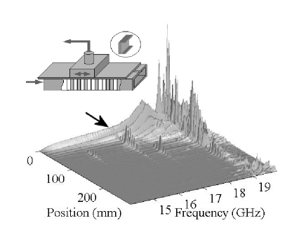
Figure 1: Spectra of the field amplitude at each point along a typical random sample normalized to the amplitude of the incident field. The arrow points to the input direction. Inset: Description of the experimental set up and schematic of the ceramic structure element.

Field spectra are taken along the length of a slotted W-42 microwave waveguide using a vector network analyzer. The field is weakly coupled to a cable without a protruding antenna inside a copper enclosure. A 2 mm-diameter hole in the enclosure is pressed against the slot, which is otherwise covered by copper bars attached to both sides of the enclosure (inset Fig. 1). The entire detector assembly is translated in 1 mm steps by a stepping motor. Measurements are made in one hundred random sample realizations each composed of randomly positioned dielectric elements. Ceramic blocks are milled to form a binary element of length $a=7.74\pm 0.04$ mm. The first half of the block is solid and the second half comprises two projecting thin walls on either side of the air space, as shown in the inset of Fig. 1. The orientation of the solid element towards or away from the front of the waveguide is randomly selected. This structure introduces states into the band gap of the corresponding periodic structure John close to the band edges. In order to produce states in the middle of the band gap, ceramic slabs of thickness $a/2$, corresponding to the solid half of the binary elements, or Styrofoam slabs, with refractive index close to unity, are inserted randomly. The samples are composed of 31 binary elements, 5 single ceramic elements and 5 Styrofoam elements with a total length of 28.8 cm.

Spectra of the field amplitude at equally spaced points along a typical random sample configuration normalized to the amplitude of the incident field amplitude are shown in Fig. 1. A few isolated exponentially peaked localized modes with Lorentzian linewidths are seen below 18.7 GHz. Between 18.7 GHz and 19.92 GHz, lines generally overlap so that $\delta>1$ and the wave is extended. The field amplitude within the sample over a narrower frequency range in a different random configuration in which spectrally overlapping peaks are observed within the band gap, is shown in two projections in Fig. 2.

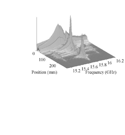
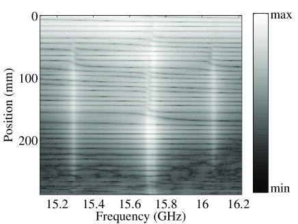
Figure 2: (a) Spectra of the field amplitude at each point along a random sample with spectrally overlapping peaks normalized to the amplitude of the incident field. (b) The top view of Fig. 2a in logarithmic presentation.

In order to exhibit the progression of the phase within the sample, a top view of the logarithm of the amplitude of the data plotted in Fig. 2a is presented in Fig. 2b. In the periodic binary structure, the same projection as in Fig. 2b, shows parallel ridges corresponding to maxima of the field amplitude separated by $a$. Thus half the wavelength equals $a$ throughout the band gap, or $\lambda$ = 2$a$. When the frequency is tuned through a Lorentzian line, which corresponds to a localized state (e.g. $\nu=15.3$ GHz), the phase through the sample increases by $\pi$ rad and an additional peak in the amplitude variation across the sample is introduced. In the frequency interval between 15.6 and 15.8 GHz where multiple peaks are observed in the field distribution, the number of ridges increases by 3.

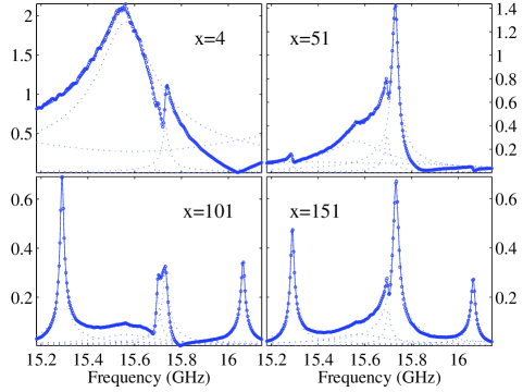
Figure 3: Comparison of the measured field magnitude (dots) to Eq. 1 (full line) at four different locations. The Lorentzian lines and the polynomial in Eq. 1 are represented in dotted lines.

This suggests that the radiation is tuned through the central frequency of three successive resonances. This is tested by fitting the field spectrum to a sum $N$ of Lorentzian lines, as follows,

$$E(\nu,x)=\sum\limits_{n=1}^{N}{\frac{A_{n}(x)}{{\Gamma_{n}(x)+i(\nu-\nu_{n}(x))}}+\sum\limits_{m=0}^{2}{C_{m}(x)(\nu-\nu_{0})^{m}}}$$ (1)

where $A_{n}(x)$ and $C_{n}(x)$ are complex coefficients. The slowly varying polynomial of the second degree centered at $\nu_{0}$ represents the sum of the evanescent wave and the tail of the response of distant lines. Here, $\nu_{0}=15.66$ GHz, which is the center of the frequency interval considered. We choose $N=5$ to include the two “satellite” lines at 15.3 GHz and 16.06 GHz. An iterative double least-squares fit procedure is applied independently at each position $x$ within the sample as follows: first guesses for the central frequencies, $\nu_{n}$, and linewidths $\Gamma_{n}$ are used to fit the spectrum measured at each position $x$ to Eq. 1 with the amplitude coefficients $A_{n}(x)$, and $C_{n}(x)$ as fitting parameters. These values are used in a second step in which, only the $\nu_{n}(x)$, and $\Gamma_{n}(x)$ are fitting parameters within a bounded spectral range. This double fitting procedure can be repeated to improve the fit. The quality of the fit can be seen in Fig. 3. Indeed, the $\chi^{2}$ normalized by the product of the integrated spectrum and degrees of freedom (the number of point minus the number of free parameters), remains below $2\times 10^{-3}$ over $90\%$ of the sample length. The noise is higher near the sample output where the signal is generally close to the noise level. The central frequencies, $\nu_{n}(x)$, and linewidths $\Gamma_{n}(x)$, found in the fit are shown in Fig. 4. A plot of the complex square of each term in Eq. 1 is shown in Fig. 5. Fluctuations in $\nu_{n}(x)$ and $\Gamma_{n}(x)$ are large only at positions for which the peak magnitude of the terms for the $n$th mode are low, as can be seen by comparing Fig. 4 and  5. In the domain in which fluctuations in the central frequencies and linewidths for a particular quasimode are low, these quantities are virtually independent of position and the field amplitude is given to good accuracy by substituting the average values of $\nu_{n}(x)=\nu_{n}$ and $\Gamma_{n}(x)=\Gamma_{n}$ in Eq. 1. The drift is greatest in mode 2, where the variation in $\nu_{2}(x)$ is less than 20% of $\Gamma_{2}$.

With $\nu_{n}$ and $\Gamma_{n}$ specified, each of the Lorentzian terms in Eq. 1 corresponds to a quasimode. The Fourier transform of each term gives the response to an incident pulse in which the temporal and spatial variation factorize, $f_{n}(x,t)=f_{n}(x)\text{exp}(-i(2\pi\nu_{n}-i\Gamma_{n})t)$ corresponding to a sum of exponentially decaying quasimodes. The independent decay of the quasimodes indicates that they are orthogonal.

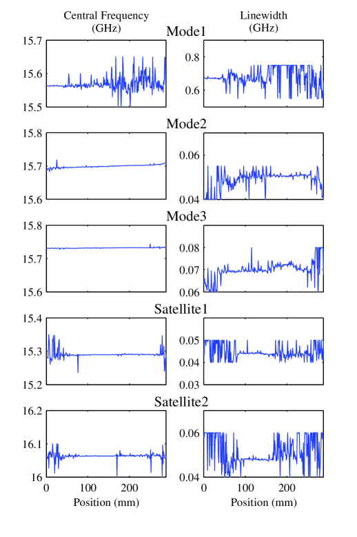
Figure 4: Spatial dependence of central frequency and linewidth for the five modes shown in Fig. 5. At positions at which the mode amplitude is greater than the noise, the central frequency and linewidth are sharply defined.

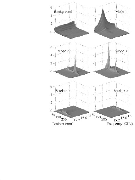
Figure 5: Field magnitude for five quasimodes and slowly varying polynomial term in Eq. 1.

For the three spectrally overlapping modes, “mode 1” ($\nu_{1}\simeq 15.56$ GHz, $\Gamma_{1}\simeq 0.67$ GHz) is broad as a result of its closeness to the input. “Mode 2” ($\nu_{2}\simeq 15.70$ GHz, $\Gamma_{2}\simeq 0.051$ GHz) and “mode 3” ($\nu_{3}\simeq 15.73$ GHz, $\Gamma_{3}\simeq 0.07$ GHz) are spatially extended and multi-peaked in a spectral range in which quasimodes are otherwise strongly localized. In fact, ”satellite modes” are not strictly localized due to the overlap with other modes. The sharply defined modes appearing in the expansion of Eq. 1 in the regions in which the amplitude of specific modes is greater than the noise in the measured field and the excellent fit to the spectra shown in Fig. 3 is consistent with these modes representing a complete set even when they overlap.

Because of dissipation within and leakage from the random sample, the system is not Hermitian, but it remains symmetric since reciprocity is preserved. A non-Hermitian but symmetric Hamiltonian has complex orthogonal eigenvalues when the appropriate inner product is used. Ching ; Weaver If the quasimodes found in the fit and shown in Fig. 5 were orthogonal, the linewidths of quasimodes would equal the sum of the absorption rate, $\Gamma_{a}$ and the leakage rates for specific modes, $\Gamma_{ln}$, for the $n$th quasimode. The sample dissipation rate is given by the ratio of the net flux into the sample, which is the difference between the incident flux and the sum of the reflected and transmitted fluxes, and the steady-state electromagnetic energy in the sample, which is proportional to $\int_{0}^{L}\epsilon(x)E^{2}dx$. Here $\epsilon(x)$ is the effective relative permittivity determined by matching the measured frequencies of the modes at the band edge of the periodic structure with the results of one-dimensional model and including waveguide dispersion. $\Gamma_{ln}$ is determined from the ratio of flux away from the sample for a given quasimode to the energy in the sample for this quasimode for steady-state excitation. The leakage from the sample for a given quasimode is obtained by decomposing the scattered wave in the empty waveguide before and after the random sample into a sum of Lorentzian lines as given in the first sum on the right hand side of Eq. (1) . The flux is then proportional to the product of the square of the amplitude of this field component and the group velocity in the waveguide. Within experimental uncertainty of 25$\%$, we find that the mode linewidths are equal to the sum of the absorption and leakage rates. This is consistent with the conclusion that quasimodes found are orthogonal.

In conclusion, we have shown that the field inside an open dissipative random single-mode waveguide can be decomposed into a complete set of quasimodes, even when the mode spacing is comparable to the linewidths. Smaller mode spacing do not occur for spatially overlapping mode because of mode repulsion. We find a multi-peaked extended field distribution whenever quasimodes overlap, and a single peaked field distribution in the rare cases of spectrally isolated modes. Because absorption suppresses long-lived single-peaked states more strongly than short-lived multiply peaked states, wave penetration into the second half of the sample and transmission through the sample are substantial only when a number of closely spaced quasimodes are excited. Though waves may extend through the sample when quasimodes overlap in a spectral range in which $\delta<1$, their envelope still falls exponentially near each peak representing a center of localization and the nature of transport may still be differentiated from diffusive regions for which $\delta>1$. The demonstration that quasimodes are well-defined when the spacing between their central frequencies is comparable to their linewidth, suggests that a quasimode description may also be appropriate for diffusing waves in samples with $\delta>1$.

We thank H. Rose, Z. Ozimkowski and L. Ferrari for suggestions regarding the construction of the waveguide assembly, and V. Freilikher, J. Barthelemy, L. Deych, V.I. Kopp, O. Legrand, A.A Lisyansky, F. Mortessagne, and R. Weaver for valuable discussions. This research is sponsored by the National Science Foundation (DMR0205186), by a grant from PSC-CUNY, by the CNRS (PICS $\#2531$) and is supported by the Groupement de Recherches IMCODE.

References

- (1) P.W. Anderson, Phys. Rev. 109, 1492 (1958).
- (2) D.J. Thouless, Phys. Rev. Lett. 39, 1167 (1977).
- (3) E. Abrahams et.al., Phys. Rev. Lett. 42, 673 (l979).
- (4) A.Z. Genack, Europhys. Lett. /bf 11, 733 (1990).
- (5) M. Ya. Azbel, Solid State Commun. 45 527 (1983).
- (6) V.D. Freilikher and S.A. Gredeskul, in Progress in Optics 30, 137 (1992).
- (7) N.F. Mott, Phil. Mag.,22, 7 (1970).
- (8) J.B. Pendry, J. Phys. C 20,733 (1987).
- (9) J.B. Pendry, Adv. Phys. 43, 461 (1994).
- (10) J. Bertolotti et.al., Phys. Rev. Lett. 94, 113903 (2005).
- (11) V. Milner, A.Z. Genack, Phys. Rev. Lett. 94, 073901 (2005).
- (12) I.M. Lifshits, and V.Ya. Kirpichenkov, Zh. Eksp. Teor. Fiz. 77, 989 (1979) [Sov. Phys. JETP 50, 499 (1979)].
- (13) L.I. Deych et.al., Phys. Rev. E, 57, 7254 (1998).
- (14) S. He and J.D. Maynard, Phys. Rev. Lett. 57, 3171 (1986).
- (15) K. Petermann, IEEE J. Quant. Electon. 15, 566 (1979).
- (16) A.E. Siegman, Phys. Rev. A 39,1253 (1989).
- (17) E.S.C. Ching et.al., Rev. Mod. Phys. 70, 1545 (1998).
- (18) S.M. Dutra and G. Nienhuis, Phys. Rev. A 62, 063805 (2000).
- (19) H. Schomerus et.al., Physica A 278, 469 (2000).
- (20) S. John, Phys. Rev. Lett. 58, 2486 (1987).
- (21) U. Kuhl et.al., J. Phys. A: Math. Gen. 38, 10433 (2005).