Mapping of the Anisotropic Two-channel Anderson Model             onto a Fermi-Majorana bi-Resonant Level Model

Abstract

We establish the correspondence between an extended version of the two-channel Anderson model and a particular type of bi-resonant level model. For certain values of the parameters the new model becomes quadratic. We calculate in closed form the entropy and impurity occupation as functions of temperature and identify the different physical energy scales of the problem. We show how, as the temperature goes to zero, the model approaches a universal line of fixed points non-Fermi liquid in nature.

The challenge of single impurity models has a long history that started some four decades ago with the study of the single-channel Kondo model kondo1964 . The strongly-coupled physics of its low temperature regime was determinant in the need to employ non-perturbative techniques to unravel the physics and the nature of the infrared fixed point. The landmark achievements in this respect were the numerical renormalization group study of Wilson wilson1975 and the Bethe ansatz solution of Andrei and Wiegmann andrei1980 ; wiegmann1980 on one hand, and the identification by Toulouse toulouse1969 ; schlottmann1978 of a solvable point of the anisotropic version of the model on the other hand. These three techniques are special, because they allow the study of the crossover regime leading to the unambiguous identification of the strongly-coupled Fermi-liquid fixed point of the model. These tools were subsequently successfully applied to more general models incorporating valence fluctuations Hewson , or multiple channels and non-Fermi-liquid characteristics cox1998 ; the next logical step was to consider models incorporating both elements simultaneously in order to understand their interplay.

The ideas behind the two-channel Anderson model were first introduced in an attempt to model the non-Fermi-liquid physics of certain U-based heavy fermions like the UBe₁₃ compound cox1987 . Its relationship to the two-channel Kondo model Nozieres1980 is as in the case of the respective single-channel models: it not only captures the local moment physics and provides a physical mechanism for moment formation, but at the same time describes also other regimes in which mixed valence prevails all the way down to the lowest temperatures. This is of great relevance because a large number of compounds are believed to be near mixed valence and therefore a good understanding of the full Anderson model physics should prove instrumental in the description of their phenomenology cox1998 . Whereas the outermost $f$-shell of, for instance, Ce ions in typical heavy-Fermion compounds is usually singly occupied, that of U ions is believed to fluctuate between the $5f^{2}$ and $5f^{3}$ valence states. A minimal model that takes into account spin-orbit and crystal-field effects leads to modeling those two states with $\Gamma_{3}$ (flavor) and $\Gamma_{6}$ (spin) doublets that hybridize with $\Gamma_{8}$ conduction electrons cox1998 .

On the other hand, the quest to a better understanding of non-Fermi-liquid physics has recently permeated into the field of mesoscopics and there are several attempts at realizing two-channel Kondo physics in the controlled and highly-tunable realm of quantum dots berman1999 ; oreg2003 ; shah2003 . Realizations based on the two-channel Anderson model may allow for a more robust description of certain aspects of the physics of such devices, like the charge fluctuations behind their capacitance lineshapes bolech2005b .

Among the different non-perturbative techniques mentioned above, bosonization –or Coulomb gas– based mappings occupy a singular place Giamarchi . Their appeal is due to the elegance of the solution and the simplicity of the picture that emerges from them; these qualities are invaluable in providing an intuitive understanding of the physics and render them complementary to more involved techniques like Bethe ansatz afl1983 or numerical renormalization group wilson1975 . In this letter, we present a mapping between the anisotropic two-channel Anderson impurity model and a resonant-level Hamiltonian that for particular values of the parameters becomes non-interacting. This property is analogous to the so-called Toulouse point of the single-channel Kondo problem toulouse1969 ; schlottmann1978 , but displays characteristics of non-Fermi-liquid physics like in the Emery-Kivelson mapping for the two-channel Kondo problem emery1992 ; fabrizio1995 ; schofield1997 ; ye1997 ; vondelft1998 . Moreover, our mapping of the two-channel Anderson model fully captures also the physics of mixed valence, something achieved previously only in the infinite-$U$ single-channel case kotliar1996 . We confirm, in a very compact unified language, all the predictions made recently for the model using a variety of other non-perturbative techniques schiller1998 ; bolech2002 ; johannesson2003 ; anders2005 ; jba2005 ; bolech2005a . We identify the two crossover energy scales of the model, below which the physics is governed by a line of non-Fermi-liquid fixed points. We are able to calculate both dynamical and thermodynamical quantities of interest over the full temperature range, across both crossovers, and connect explicitly all different high temperature regimes with the zero-temperature line of fixed points.

We are thus lead to consider the following generalization of the two-channel Anderson Hamiltonian, $H=H_{\text{host}}+H_{\text{i+h}}+H_{3}\,$. The first two terms correspond: to the band electrons ($\psi_{\alpha\sigma}^{\dagger}$) the first one,

$$H_{\text{host}}=\sum_{\alpha\sigma}\int dx~{}\psi_{\alpha\sigma}^{\dagger}\left(x\right)\left(-i\partial_{x}\right)\psi_{\alpha\sigma}\left(x\right)~{}\text{,}$$ (1)

and to the impurity ($X_{ab}$) the second one,

$$H_{\text{i+h}}=\varepsilon_{s}\sum_{\sigma}X_{\sigma\sigma}+\varepsilon_{f}\sum_{\alpha}X_{\bar{\alpha}\bar{\alpha}}+\\ +V\sum_{\alpha\sigma}\left[X_{\sigma\bar{\alpha}}\psi_{\alpha\sigma}\left(0\right)+\psi_{\alpha\sigma}^{\dagger}\left(0\right)X_{\bar{\alpha}\sigma}\right]~{}\text{.}$$ (2)

Taken toghether they constitute the standard two-channel model. Here we have described the Hilbert space of the impurity using Hubbard-operator notation, $X_{ab}=\left|a\right\rangle\left\langle b\right|$, where $a,b=\left(\sigma=\uparrow,\downarrow\right),\left(\bar{\alpha}=\bar{+},\bar{-}\right)$. The third term, $H_{3}=\sum_{\nu}H_{3}^{\nu}$, involving density-density interactions in the different sectors ($\nu$), is mainly added to break the two $SU\left(2\right)$ symmetries in spin and flavor, introducing anisotropy as is standard in RG and Coulomb-gas analysis. The impurity densities involved are

$$X_{c}=X_{s\!f}=\sum_{\sigma}X_{\sigma\sigma}-\sum_{\alpha}X_{\bar{\alpha}\bar{\alpha}}~{}\text{,}$$ (3)

$$X_{s}=\sum_{\sigma}\sigma X_{\sigma\sigma}~{}\text{,\qquad\qquad\qquad}X_{f}=\sum_{\alpha}\alpha X_{\bar{\alpha}\bar{\alpha}}~{}\text{.}$$

The corresponding terms in the charge ($c$), spin ($s$), flavor ($f$), and spin-flavor ($s\!f$) sectors are

$$H_{3}^{\nu}=J_{\nu}^{3}X_{\nu}\sum_{\alpha\sigma\alpha^{\prime}\sigma^{\prime}}\psi_{\alpha\sigma}^{\dagger}\left(0\right)\Upsilon_{\alpha\sigma,\alpha^{\prime}\sigma^{\prime}}^{\nu}\psi_{\alpha^{\prime}\sigma^{\prime}}\left(0\right)~{}\text{,}$$ (4)

where

$$\begin{array}[c]{lll}\Upsilon_{\alpha\sigma,\alpha^{\prime}\sigma^{\prime}}^{c}=\delta_{\alpha\alpha^{\prime}}\delta_{\sigma\sigma^{\prime}}~{}\text{,}&&\Upsilon_{\alpha\sigma,\alpha^{\prime}\sigma^{\prime}}^{s}=\delta_{\alpha\alpha^{\prime}}\tau^{3}{}_{\sigma\sigma^{\prime}}~{}\text{,}\\ \Upsilon_{\alpha\sigma,\alpha^{\prime}\sigma^{\prime}}^{f}=\tau^{3}{}_{\alpha\alpha^{\prime}}\delta_{\sigma\sigma^{\prime}}~{}\text{,}&&\Upsilon_{\alpha\sigma,\alpha^{\prime}\sigma^{\prime}}^{s\!f}=\tau^{3}{}_{\alpha\alpha^{\prime}}\tau^{3}{}_{\sigma\sigma^{\prime}}~{}\text{,}\end{array}$$ (5)

and $\tau^{3}$ is the third Pauli matrix.

Many times, the physics of (1+1)-dimensional models is more transparent in a bosonic representation Giamarchi . The bosonization prescription reads $\psi_{\alpha\sigma}\left(x\right)\approx e^{-i\phi_{\alpha\sigma}\left(x\right)}/\sqrt{2\pi a}$, with $a$ a regulator that goes to zero in the continuum limit . It is convenient to change basis in the bosonic fields according to $\phi_{\alpha\sigma}=(\phi_{c}+\sigma\phi_{s}+\alpha\phi_{f}+\alpha\sigma\phi_{s\!f})/2$. Even more, we find that remarkable simplifications are achieved by performing the canonical transformation $U=\prod\nolimits_{\nu}e^{i\gamma_{\nu}\phi_{\nu}\left(0\right)X_{\nu}}$, with $2\gamma_{c}=\gamma_{s}=-\gamma_{f}=2\gamma_{s\!f}=1/2$. This unitary transformation is a generalization of the one used in the study of Kondo-type impurity exchange models. By choosing $J_{\nu}^{3}=\pi\gamma_{\nu}$, the first and third terms of the Hamiltonian yield

$$U\left(H_{\text{host}}+H_{3}\right)U^{\dagger}=\sum_{\nu}H_{0}^{\nu}\equiv\frac{1}{4\pi}\sum_{\nu}\int dx~{}\left(\partial_{x}\phi_{\nu}\left(x\right)\right)^{2}$$

On the other hand, the impurity terms become

$$UH_{\text{i+h}}U^{\dagger}=\varepsilon_{s}\sum_{\sigma}X_{\sigma\sigma}+\varepsilon_{f}\sum_{\alpha}X_{\bar{\alpha}\bar{\alpha}}+\\ +\frac{V}{\sqrt{2\pi a}}\left[\left(X_{\uparrow\bar{+}}+X_{\downarrow\bar{-}}\right)+e^{i\phi_{s\!f}}\left(X_{\uparrow\bar{-}}+X_{\downarrow\bar{+}}\right)+\text{H.c.}\right]~{}\text{.}$$

We can next refermionize the model introducing the fermionic operators $f=X_{\bar{-}\bar{+}}+X_{\uparrow\downarrow}$ and $d=e^{-i\pi f^{\dagger}\!f}\left(X_{\uparrow\bar{-}}+X_{\downarrow\bar{+}}\right)$, plus the new prescription $\psi_{\nu}\left(x\right)\approx e^{-i\pi\left(f^{\dagger}\!f+d^{\dagger}\!d\right)}e^{-i\phi_{\nu}\left(x\right)}/\sqrt{2\pi a}$. We find that the impurity couples only to the spin-flavor sector and the physics is governed by the following Fermi-Majorana bi-resonant level model (see also Fig. 1):

$$H_{\text{biRes}}=H_{0}^{s\!f}-\varepsilon~{}d^{\dagger}\!d+\varepsilon_{s}+\\ +\sqrt{2\Delta}\left[\psi_{s\!f}^{\dagger}\left(0\right)d+d^{\dagger}\psi_{s\!f}\left(0\right)\right]+\\ +\sqrt{2\Gamma}\left(f^{\dagger}-f\right)\left(d^{\dagger}+d\right)~{}\text{,}$$ (6)

where $\varepsilon=\varepsilon_{s}-\varepsilon_{f}$, $\Delta=V^{2}/2$ and $\Gamma=\Delta/2\pi a$. This is a purely quadratic model, on which reintroducing the terms with non-zero $\lambda_{\nu}=\gamma_{\nu}-J_{\nu}^{3}/\pi$ would parametrize the deviations from the solvable point (cf. Refs. [clarke1993, ; sengupta1994, ]). It is interesting to point out the similarities and differences between this model and the Majorana resonant-level model that corresponds to the solvable point of the two-channel Kondo model emery1992 . In both cases the impurity hybridizes only with $\psi_{s\!f}^{\dagger}$, but for the Anderson case the situation is more complex: two fermionic degrees of freedom are required to represent the impurity. One ($d^{\dagger}$) with a chemical potential $\varepsilon$ that vanishes at the intrinsic mixed-valence point and goes off-resonance in the local-moment regimes. A second one ($f^{\dagger}$) –related to the spin and flavor fluctuations– that couples only via one of its Majorana components and is always resonant in the absence of external fields. As in the Kondo case, the other Majorana component of $f^{\dagger}$ exists completely decoupled from the rest of the system and will be responsible for the fractional residual impurity entropy that we discuss below.

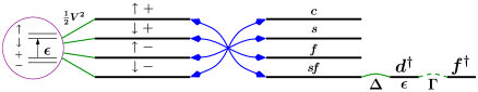
Figure 1: Pictorial representation of the anisotropic two-channel Anderson impurity model before (right) and after (left) the mapping onto a Fermi-Majorana bi-resonant level model.

It is a relatively simple task to extract the impurity thermodynamics and correlation functions at the solvable point. The impurity free energy can be conveniently computed using Pauli’s trick of integrating over the coupling constants. After some algebra, one arrives at

$$\Omega-\Omega_{0} =\int_{0}^{1}\frac{d\lambda}{\lambda}~{}\left\langle\lambda\left(H_{\text{biRes}}-H_{0}^{s\!f}\right)\right\rangle_{\lambda}$$

$$=-\int_{0}^{1}d\lambda~{}\frac{1}{\beta}\sum_{n\geq 0}\frac{\partial_{\lambda}D\left(\omega_{n},\lambda\right)}{D\left(\omega_{n},\lambda\right)}~{}\text{,}$$ (7)

where

$$D\!\left(\omega,\lambda\right)=\lambda^{4}\!\left(8\Gamma\Delta+\Delta^{2}\omega\right)+\lambda^{2}\!\left(8\Gamma\omega+\varepsilon^{2}\omega+2\Delta\omega^{2}\right)+\omega^{3}$$

and $\omega_{n}=\pi(2n+1)/\beta$ are fermionic Matsubara frequencies. Introducing a suitable regularization that can be removed later from the actual physical quantities, one computes the different magnitudes of interest. In particular, the impurity entropy is given by $S-S_{0}=\sum_{k}s\left(z_{k}\right)$ with

$$s\left(z\right)=z\left[\psi\left(\frac{1}{2}+z\right)-1\right]-\ln\Gamma\left(\frac{1}{2}+z\right)+\frac{1}{2}\ln\pi$$ (8)

and $\psi\left(z\right)$ the digamma function. Here $z_{k}=-\beta\omega_{k}/2\pi$, with $\omega_{k=0,1,2}$ the three roots of $D\!\left(\omega,1\right)$. One finds that in the physical regime $\omega_{0}$ is real while $\omega_{1,2}$ are complex conjugate of each other. That prompts us to identify the Kondo and Schottky temperature scales:

$$T_{\text{K}}\equiv-\omega_{0}/2\pi k_{\text{B}}\quad<\quad T_{\text{S}}\equiv\left|\omega_{1}\right|/2\pi k_{\text{B}}~{}\text{,}$$ (9)

so that

$$S-S_{0}=s\left(T_{\text{K}}/T\right)+\left[\text{Schottky contribution}\right]$$ (10)

Remarkably, the function $s\left(z\right)$ is the same as that found for the entropy of the two-channel Kondo model at the Emery-Kivelson point fabrizio1995 . This is not completely unexpected, since Kondo is the low energy effective theory for most part of the parameter regime of the two-channel Anderson model.

Figure 2: Impurity contribution to the entropy as a function of temperature for different values of $\varepsilon$ ($0$, $\pm 2$, $\pm 4$, $\pm 6$, $\pm 8$). The solid lines correspond to the results for the soluble point after identification of the scales with the ones of the isotropic model. For the sake of contrast, the corresponding curves for the latter are shown with dashed lines for the same set of values of $\varepsilon$.

For the sake of illustration, in Fig. 2, we show the impurity contribution to the entropy as a function of temperature for the full range. For the purpose of this figure, we have identified the two scales with those of the isotropic model bolech2002 , which allows us to conveniently display in the same plot the results for the latter. The figure illustrates how, for large $\left|\varepsilon\right|$, the entropy of the impurity is quenched in two stages as the temperature is lowered: $k_{\text{B}}\ln 4\rightarrow k_{\text{B}}\ln 2\rightarrow k_{\text{B}}\ln\sqrt{2}$. For small $\left|\varepsilon\right|$, the two quenching steps coalesce on a single one. In all cases, the final value of the entropy is the same, and indicative of the non-Fermi-liquid character of the zero-temperature fixed points. Notice that the main difference between the curves for the isotropic model and those for the anisotropic one at the soluble point, reside in the shape of the second, or Kondo, quenching step. This difference could be traced back to the absence of the leading irrelevant operators at the soluble point (cf. with the same situation in the case of the two-channel Kondo model). In the language of specific heats, the $T\ln T$ leading terms are absent from the soluble anisotropic model and can be recovered using perturbation theory in $\lambda_{\nu}$ (cf. Refs. [emery1992, ; sengupta1994, ]). The same holds true for the leading logarithms in the magnetic and flavor susceptibilities clarke1993 .

Figure 3: Normalized curves of the impurity charge valence as a function of temperature. The results for the soluble anisotropic case (solid lines) and Bethe ansatz results for the isotropic case (dashed lines) are displayed for different values of $\varepsilon$ ($\pm 2$, $\pm 4$, $\pm 6$, $\pm 8$).

Another quantity of interest is the impurity charge valence $n_{c}=\partial\Omega/\partial\varepsilon$ given by

$$n_{c}-n_{c,0}=\frac{1}{\beta}\sum_{k}\psi\left(\frac{1}{2}+z_{k}\right)\partial_{\varepsilon}z_{k}~{}\text{.}$$ (11)

This is an aspect of the physics inherent to Anderson type models and of particular relevance in their application in the context of quantum dots and other mesoscopic systems that allow direct measurements of it bolech2005b . The valence starts at $n_{c,0}=1/2$ for high temperature ($T\gg T_{\text{S}}$) and evolves to reach finally a certain zero-temperature value $n_{c}^{0}\equiv n_{c}\left(\varepsilon\right)_{T=0}$ that labels the line of fixed points of the model. Figure 3 shows normalized curves for the temperature dependence of the impurity charge valence. The quenching of the valence fluctuations takes place at the characteristic scale $T_{\text{S}}$. The correspondence between the bosonization results and the results for the isotropic case is rather good for $\left|\varepsilon\right|$ large, and the differences for small $\left|\varepsilon\right|$ are in part due to the difficulty for identifying the scales of the two models. Nevertheless, subtle aspects of the small $\left|\varepsilon\right|$ curves, like the ‘overshoot’ of the curves at intermediate temperatures $T\lesssim T_{\text{S}}$, are also present at the soluble point. All this shows that the isotropic model and the soluble anisotropic point not only share the same infrared fixed-point behavior, albeit with different irrelevant operators content, but also display matchable generic ultraviolet physics.

In summary, we have shown that the anisotropic two-channel Anderson model can be solved exactly for particular values of the coupling constants in the extra $H_{3}$ term of the Hamiltonian. Using bosonization, we demonstrated that the problem reduces to the study of a non-interacting Fermi-Majorana bi-resonant level model. Deviations from the solvable point can be taken into account using perturbation theory in, call it, $\delta H_{3}$. The advantage of the method is evident: closed analytical expressions can be derived for the full temperature crossovers of the different quantities of interest; this sets the approach apart from other non-perturbative techniques applied to the model in the past. Although the fixed point line of the solvable anisotropic case is the same as for the usual isotropic model (i.e., anisotropy is irrelevant), the leading irrelevant operator content of the anisotropic model is more restricted, –which lies behind its greater simplicity. A manifestation of this difference is found, for instance, in the results we presented for the impurity entropy. On a different front, and as compared with pure-exchange type of models like the two-channel Kondo, the Anderson model brings in as well the physics of mixed valence and charge fluctuations. We have shown that the essential aspects of this physics are again well captured by the bi-resonant level Hamiltonian. In a future contribution, we plan to give more specialized technical details of the Abelian bosonization procedure and discuss the different field susceptibilities . This work opens up multiple other possibilities for the study of two-channel Anderson models as applied to the physics of heavy-fermions and mesoscopic systems. One may, for instance, consider the behavior of more than one impurity and, in particular, the case of two-channel Anderson lattices.

- (1) J. Kondo, Prog. theor. Phys. 32, 37 (1964).
- (2) K.G. Wilson, Rev. Mod. Phys. 47, 773 (1975).
- (3) N. Andrei, Phys. Rev. Lett. 45, 379 (1980).
- (4) P.B. Wiegmann, Phys. Lett. 80A, 163 (1980).
- (5) G. Toulouse, C. R. Acad. Sci. 268, 1200 (1969). See also P.W. Anderson, G. Yuval, and D.R. Hamann, Phys. Rev. B 1, 4464 (1970).
- (6) P. Schlottmann, J. Phys. (Paris) 39, C6-1486 (1978).
- (7) A.C. Hewson, The Kondo Problem to Heavy Fermions, Cambridge University Press, Cambridge, England, 1993.
- (8) D.L.A. Cox and A. Zawadowski, Adv. in Phys. 47, 599 (1998).
- (9) D.L. Cox, Phys. Rev. Lett. 59, 1240 (1987), Erratum: ibid. 61, 1527 (1988).
- (10) P. Nozières and A. Blandin, J. Physique 41, 193 (1980).
- (11) D. Berman, N.B. Zhitenev, R.C. Ashoori, and M. Shayegan, Phys. Rev. Lett. 82, 161 (1999).
- (12) Y. Oreg and D. Goldhaber-Gordon, Phys. Rev. Lett. 90, 136602 (2003).
- (13) N. Shah and A.J. Millis, Phys. Rev. Lett. 91, 147204 (2003).
- (14) C.J. Bolech and N. Shah, Phys. Rev. Lett. 95, 036801 (2005).
- (15) T. Giamarchi, Quantum Physics in One Dimension, (Clarendon Press, Oxford, 2004).
- (16) N. Andrei, K. Furuya, and J.H. Lowenstein, Rev. Mod. Phys. 55, 331 (1983).
- (17) V.J. Emery and S. Kivelson, Phys. Rev. B 46, 10812 (1992).
- (18) M. Fabrizio, A.O. Gogolin, and P. Nozières, Phys. Rev. B 51, 16088 (1995).
- (19) A.J. Schofield, Phys. Rev. B 55, 5627 (1997).
- (20) J. Ye, Phys. Rev. B 56, R489 (1997).
- (21) J. von Delft, G. Zaránd, and M. Fabrizio, Phys. Rev. Lett. 81, 196 (1998).
- (22) G. Kotliar and Q. Si, Phys. Rev. B 53, 12373 (1996).
- (23) A. Schiller, F.B. Anders, and D.L. Cox, Phys. Rev. Lett. 81, 3235 (1998).
- (24) C.J. Bolech and N. Andrei, Phys. Rev. Lett. 88, 237206 (2002).
- (25) H. Johannesson, N. Andrei, and C.J. Bolech, Phys. Rev. B 68, 075112 (2003).
- (26) F.B. Anders, Phys. Rev. B 71, 121101(R) (2005).
- (27) H. Johannesson, C.J. Bolech, and N. Andrei, Phys. Rev. B 71, 195107 (2005).
- (28) C.J. Bolech and N. Andrei, Phys. Rev. B 71, 205104 (2005).
- (29) D.G. Clarke, T. Giamarchi, and B.I. Shraiman, Phys. Rev. B 48, 7070 (1993).
- (30) A.M. Sengupta and A. Georges, Phys. Rev. B 49, 10020(R) (1994).