Monte Carlo Simulation of Small-World Models with Weak Long-Range Interactions

Abstract

Large-scale Monte Carlo simulations, together with scaling, are used to obtain the critical behavior of the Hastings long-range model and two corresponding models based on small-world networks. These models have combined short- and long-range interactions. For all three models, the critical scaling behavior predicted by Hastings [Phys. Rev. Lett. 91, 098701] is verified.

I Introduction

Traditionally, studies of materials have concentrated on either models based on regular graphs or random graphs (such as the models on percolating lattices KIRK73 , the $z$ model SCAL91 ; NOVO05c , or the model in Ref. RAME04 ). Recently, much more attention has been paid to networks that are midway between random graphs and regular graphs, for example, scale-free networks IGLO02 . The critical behavior, as well as the transport properties, are different from that of the same model on a regular graph. The small world (SW) graph BARA02 is a type of graph that interpolates between a regular graph and a random graph. These graphs have been widely used in many areas, for example, in parallel simulations KORN03 ; KORN99 ; KORN00 ; KOLA03 ; KORN02 and in studies of the Internet BARA02 . Since a particular material is related to a given graph with interactions based on the two-body interaction approximation CHAR85 , many models of materials have been studied on small world graphs. These models include the Ising model, Heisenberg model, and random-walker models GITT00 ; BARR00 ; PEKA01 ; HONG02b ; KIM01 ; HONG02 ; HERR02 ; JEON03 ; HAST03 ; KOZM04 ; JEON05 ; KOZM05 ; NOVO04 ; NOVO05 ; NOVO05b ; NOVO05c . Such studies show that these models exhibit mean-field behavior.

It is not easy to analyze small-world models theoretically because of the randomness of the long-range bonds BARA02 . Hastings introduced a long-range model to explain the critical phenomena in small-world systems analytically HAST03 . His model, in which long-range interactions are distributed to all the spins in the system, has no randomness and is easier to analyze. He claimed that his model has the same universal behavior as the small world model, with some constrains, and presented a criterion for the crossover to the underlying mean-field behavior. Thus far, there are no experimental or computer simulation verifications of Hastings long-range model, as well as its comparision with other small-world models. In this article, Monte Carlo simulations for the $2$-dimensional Hastings model and two corresponding SW models with Ising spins are presented and the critical behavior is analyzed.

II Model and Methods

All three models studied start with a $2$-dimensional $L\times L$ square lattice with periodic boundary conditions and an Ising spin with $s_{i}\pm 1$ located on each site, and a nearest neighbor interaction constant $J$. For the first model, the small-world Ising model, randomly chosen pairs of Ising spins are connected with a bond, a fixed number ($w$) of these small-world bonds are added. Once a SW bond is added to a pair of spins, no other SW bond is allowed to be added to these spins. These SW bonds do not change during the simulation, i.e. they are quenched. So the total number of Ising spins in the model is $N=L^{2}$, and the number of SW bonds is less than $\frac{L^{2}}{2}$. Thus, the ratio of the number of small-world bonds to the regular nearest neighbor bonds is $p=\frac{w}{2L^{2}}$. On average, a spin in the system has $z=4+\frac{2w}{L^{2}}=4+4p$ nearest neighbor bonds. We suppose the interaction via SW bonds is the same strength as that via regular lattice bonds. The Ising Hamiltonian of such a system is given by

$${\cal H}=-J\sum_{\langle i,j\rangle}s_{i}s_{j}-J\sum_{\rm SW}s_{i}s_{j}\>.$$ (1)

The first sum is over the four nearest neighbor spins on the square lattice, and the second sum is over the $w$ SW bonds. We use $J=1$ in this article.

Hastings constructed his long-range model by giving each spin on the lattice a weak coupling, of order $\frac{p}{N}=\frac{p}{L^{2}}$, to every other spin in the lattice, instead of adding long-range bonds with probability $p$ HAST03 . Hence the Hastings’ Hamiltonian can be written as

$${\cal H} = -J\sum_{\langle i,j\rangle}s_{i}s_{j}-J\frac{p}{2N}\sum_{i,j\neq i}s_{i}s_{j}$$ (2)

$$= -J\sum_{\langle i,j\rangle}s_{i}s_{j}-J\frac{p}{2N}\left(N\sum_{i}Ms_{i}-N\right).\>$$

Here $M$ is the magnetization density,

$$M=\frac{1}{N}\sum_{i}s_{i}\>.$$ (3)

We utilized standard Monte Carlo (MC) simulations LAND00 . A Glauber flip probability with the site for an attempted update chosen at random is used. In our implementation, two random numbers, $r_{1},r_{2}$, are generated. The first number is used to randomly choose a spin for the spin flip attempt, the second is used to determine whether the chosen spin should be flipped. If

$$r_{2}\leq\frac{\exp^{-E_{\rm new}/k_{\rm B}T}}{\exp^{-E_{\rm old}/k_{\rm B}T}+\exp^{-E_{\rm new}/k_{\rm B}T}}\>,$$ (4)

the chosen spin will be flipped. Here $T$ is the temperature and $k_{\rm B}$ is Boltzmann’s constant (in our units $k_{\rm B}$$=$$1$). The current energy is $E_{\rm old}$ and $E_{\rm new}$ is the energy if the chosen spin is flipped.

We also study another small-world model, one with annealed SW bonds. The model is on the square lattice, with a long-range interaction the same as the regular lattice interaction $J$. At each Monte Carlo spin flip trial, randomly choose a spin and for this one update attempt, add with probability $p$ a small-world connection between this spin and another randomly chosen spin. Calculate the energies $E_{\rm old}$ and $E_{\rm new}$ using the four square-lattice nearest neighbor spins and the small-world connection (if it is added), with use of Eq. (4), flip the chosen spin. This Monte Carlo process is similar to the spin-exchange process used by Rácz et al RACZ90 ; RACZ91 . Since the long-range random connection is annealed in this model, we call this model the annealed small-world model.

The Monte Carlo simulation is performed on a parallel computer with each processing element running a particular temperature for systems with size less than $N=256^{2}$, while up to four processing elements running a particular temperature for the largest system size $N=384^{2}$. The SPRNG SPRNG random number generator is used. A number of quantities are measured, but only the order parameter ($|M|$) and the Binder $4$th order cumulant ($U_{4}$) are reported here, $|M|=\frac{1}{NK}\sum_{j=1}^{K}\left|\sum_{i=1}^{N}s_{i}\right|_{j}$ and $U_{4}=1-\frac{\left\langle M^{4}\right\rangle}{3\left\langle M^{2}\right\rangle^{2}}$. The summation index $j$ runs over the $K$ different configurations generated in the Monte Carlo simulation. Up to 128 processing elements were used in our simulations. It took about $40$ hours per data run for system size $N=256^{2}$ and $70$ hours for system size $N=384^{2}$. For each temperature, averages are taken using $K$$=$$10^{6}$ Monte Carlo Steps per Spin (MCSS).

Hastings developed a general scaling method by using renormalization group theory combined with mean-field techniques for small world systems. He predicted that for small-world systems with small $p$, the critical point shifts away from the Ising critical point, from Eq. (9) in HAST03 ,

$${\widetilde{T}}_{c}-T_{c}=A_{t}p^{1/\gamma}\>.$$ (5)

Here $\gamma$ is the critical exponent for the susceptibility for the local regular lattice system, $\widetilde{T}_{c}$ is the critical temperature of SW system, and $T_{c}$ is the critical temperature of the local system. Here the local system is a $2d$ square Ising lattice, so $T_{c}=2.2691\cdots$. The prefactor $A_{t}=(A_{\chi}^{+})^{1/\gamma}$, where $A_{\chi}^{+}$ is the prefactor in the scaling of the susceptibility $\chi$. It is also predicted that below the critical point, $T<\widetilde{T}_{c}$, the magnetization in the limit $N\rightarrow\infty$ is (from Eq. (10) in HAST03 )

$$|M|=A_{M}{\widetilde{T}}_{c}^{\frac{1}{2}}\left(1-\frac{T}{{\widetilde{T}}_{c}}\right)^{\frac{1}{2}}\left({\widetilde{T}}_{c}-T_{c}\right)^{\beta-\frac{1}{2}}\>.$$ (6)

Here $A_{M}$ is a prefactor and $\beta$ is the critical exponent for the order parameter for the local regular lattice system. In the models studied in this article, the local system is a $2d$ Ising model, so $\beta=\frac{1}{8}$ and $\gamma=\frac{7}{4}$. Hence $|M|={\widetilde{A}}\sqrt{\widetilde{T}_{\rm c}-T}$ for $T<\widetilde{T}_{\rm c}$, and the mean field amplitude $\widetilde{A}\propto p^{\frac{\beta-\frac{1}{2}}{\gamma}}$ diverges as the long-range interaction strength $p$ (or the ratio of SW bonds to regular lattice bonds $p$) approaches zero. The mean field region for this scaling is small HAST03 , with mean field behavior only over a region given by

$$|T_{\rm c}-T|\propto p^{\frac{1}{\gamma}}\propto|T_{\rm c}-{\widetilde{T}}_{\rm c}|\>.$$ (7)

Note that this type of scaling is related to the coherent anomaly method pioneered by Suzuki MSUZ95 . Also, this scaling can only be expected to be seen in systems with a small amount of long-range interactions ($p$ small). For SW systems with a large amount of long-range bonds ($p=0.25$), even if the long-range interaction is weak ($0.01J,\>0.05J,\>0.1J,\>0.5J$), this predicted scaling was not observed NOVO05c for the system sizes we studied.

For small $p$, as the system size increases, the crossing point of $U_{4}$ approaches the point where $U_{4}$ is the predicted value for infinite size mean field models, $U_{4,\infty}^{\rm(MF)}=0.2705\cdots$ NOVO05c ; BREZ85 . We use the temperature where $U_{4}=U_{4,\infty}^{\rm(MF)}$ as the estimate for the critical temperature $\widetilde{T}_{\rm c}$ in our scaling.

III Results and Scaling

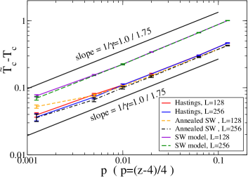
Figure 1: (color online) The critical temperature relation from Eq. (5). The critical temperature of the Hastings model is much smaller than that of the corresponding $2d$ SW model (upper curves), but very close to that of the annealed SW model. The data show that Hastings’ prediction about the critical temperature works well.

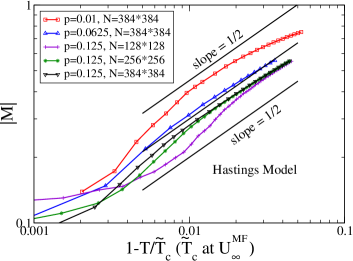
Figure 2: (color online) The order parameter $|M|$ vs. $t=1-\frac{T}{\widetilde{T}_{\rm c}}$ for the Hastings long-range model.

Simulations were performed for $p=0.00125,\>0.005,\>0.01,\>0.0625$ and $0.125$ for the Hastings model and the annealed small-world model. For the $2d$ SW model, simulations were performed for $z=4.005,\>4.02,\>4.04,\>4.254$ and $4.5$, which correspond to the above $p$ values. The results show that the critical temperature for the $2d$ SW model is larger than that for the Hastings model for the same $p$. That is what is expected since the spreading of pair-wise long-range interactions to every spin in the system weakens the long-range effect. The critical temperature for the annealed SW model is a little bit smaller than that of the Hastings model. Fig. (1) shows the critical temperature relation from Eq. (5) for all these three models, as well as the theoretical prediction. For each model, the data falls on a straight line of the Hastings predicted slope of $\frac{1}{\gamma}$. The small deviation from the slope of $\frac{1}{\gamma}$ for the smaller values of $p$ is due to fluctuations and statistical uncertainty. For the Hastings long-range model, the error estimate from $16$ independent samples for $p=0.00125$ is $\sigma=0.0030$ for $N=128^{2}$ and $\sigma=0.0045$ for $N=256^{2}$. The error estimates for the other systems is of the same order.

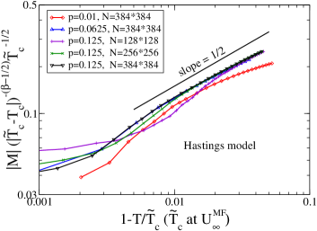
Figure 3: (color online) The order parameter scaling from Eq. (6) for the Hastings long-range model.

Fig. (2) is the simulation result for the order parameter vs. the reduced temperature $t$, where $t=1-\frac{T}{\widetilde{T}_{\rm c}}$, for the Hastings model. Only the branches for $T<\widetilde{T}_{\rm c}$ are shown. It can be seen from the figure, the data curve for $N=384^{2}$ and $p=0.125$ approaches a slope $\frac{1}{2}$ line in the region near $t<0.04$, which is consistant with the estimate from Eq. (7) (for $p=0.125$, and the largest system size we studied, $N=384^{2}$, $\widetilde{T}_{\rm c}=2.734$). The deviation from the slope of $\frac{1}{2}$ at small $t$ is due to finite size effects. This is seen by comparing systems for $p=0.125$, the smaller lattices ($N=128^{2}$ and $256^{2}$) deviate from the $N=384^{2}$ data at small $t$. For a fixed value of $N$, the region with the expected slope of $\frac{1}{2}$ is also not seen for values of $p$ that are too small (as for $N=384^{2}$ and $p=0.01$). Consequently, the prediction of Hastings HAST03 with a slope of $\frac{1}{2}$ is only seen for large enough values of $N$ and values of $p$ which are small (but not too small for a fixed $N$).

Fig. (3) to Fig. (5) are scaling results for the order parameter $|M|$ using Eq. (6) for the Hastings model, the annealed SW model, and the SW model. From Eq. (7), the mean field critical region is proportional to $\widetilde{T}_{\rm c}-T_{\rm c}$. The smaller the $p$ value, the smaller is $\widetilde{T}_{\rm c}-T_{\rm c}$ and the narrower is the mean field critical region HAST03 . In the mean field region, the scaled data points collapse to a line of slope $\frac{1}{2}$. For the Hastings model, shown in Fig. (3), the scaled data points fall on a region close to a line of slope $\frac{1}{2}$ near $t=1-\frac{T}{\widetilde{T}_{\rm c}}=0.01$ for all $p$ for larger $N$, and expands beyond $t=0.02$ on the upper side and $0.008$ on the lower side for values of $p$ that are larger ($p=0.0625$ and $0.125$). The annealed SW model and the SW model present the same behavior, Fig. (4) and Fig. (5). It is expected that, for a fixed size system, the mean field region will be wider as $p$ increases (but is still small enough so that the long-range interaction is weak). The scaling result for the $2d$ SW model illustrates this. In Fig. (5), for system size $N=384^{2}$, the mean field region of the largest value of $p=0.125$ expands much further to smaller $t$ than that of $p=0.0625$ and $p=0.01$. For a fixed $p$, the mean field region is wider for larger size systems. In Fig. (3), Fig. (4) and Fig. (5), for $p=0.125$, as the system size increases from $N=128^{2},256^{2}$ to $N=384^{2}$, the mean field region extends to smaller $t$, or, to the area where the temperature $T$ is very close to the critical temperature $\widetilde{T}_{\rm c}$. But for much smaller values of $p$, for example, $p=0.01$, the mean field region is hardly seen even for $N=384^{2}$. Simulations for larger size systems are needed to penetrate the mean field region as Hastings predicted HAST03 for much smaller $p$. Unfortunately, we can not run larger size systems due to computer limits.

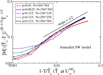
Figure 4: (color online) The order parameter scaling from Eq. (6) for the annealed SW model.

From the above analysis, the mean field region predicted by Hastings HAST03 for the order parameter is seen for large enough values of $N$ and values of $p$ which are small (but not too small for a fixed $N$) in all three Ising models we studied, the Hastings model, the annealed SW model and the SW model. It is hard to say for which model Eq. (6) works better. Although for $p=0.125$ and $N=384^{2}$, these models present a reasonable scaling result, the scaling result for a smaller $p$, here $p=0.01$, is not good and the mean field region is not obvious for our system sizes and statistics. It can not be determined whether this deviation from the predicted scaling is due to fluctuations or to finite size effects or some combination.

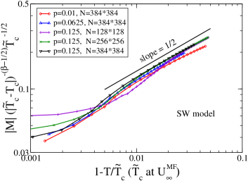
Figure 5: (color online) The order parameter scaling from Eq. (6) for the $2d$ SW model.

IV Discussion and Conclusions

Starting from the square lattice Ising model, we constructed a small-world Ising model and an annealed small-world model that have the same critical behavior as the Hastings long-range model. These two Ising models have been simulated, as well as the Hastings model. Hastings’ predictions for the critical temperature and the order parameter scaling HAST03 are verified. Results show the predicted scaling relation in HAST03 for the critical point $\widetilde{T}_{\rm c}$, Eq. (5), works well for all three models, Fig. (1). The mean field behavior predicted by Hastings HAST03 , Eq. (6), is seen in the mean field region, Eq. (7), for system sizes $N=256^{2},N=384^{2}$ and not too small $p$ ($p=0.0625$ and $0.125$), Fig. (3), Fig. (4) and Fig. (5). To see whether Hastings’ predictions work for much smaller $p$ (for example, $p\sim 0.01$), simulations for much larger size systems ($N>>384^{2}$) and much higher statistics would be required.

V Acknowledgements

We acknowledge useful discussions with a number of people, particularly Gyorgy Korniss, Per Arne Rikvold, and Zoltan Toroczkai. Supported in part by NSF grants DMR-0120310, DMR-0113049, DMR-0426488, and DMR-0444051. Computer time from the Mississippi State University High Performance Computing Collaboratory (HPC²) was critical to this study.

References

- (1) S. Kirkpatrick, Rev. Mod. Phys. 45, 574 (1973).
- (2) R.T. Scalettar, Physica A170, 282 (1991).
- (3) X. Zhang and M.A. Novotny, Braz. J. Phys., in press.
- (4) A. Ramezanpour, Phys. Rev. E 69, 066114 (2004).
- (5) F. Iglói and L. Turban, Phys. Rev. E 66, 036140(R) (2002).
- (6) R. Albert and A.-L. Barabási, Rev. Mod. Phys. 74, 47 (2002).
- (7) G. Korniss, M.A. Novotny, H. Guclu, Z. Toroczkai, and P.A. Rikvold, Science 299, 677 (2003).
- (8) G. Korniss, M.A. Novotny, and P.A. Rikvold, J. Comp. Phys. 153, 488 (1999).
- (9) G. Korniss, Z. Toroczkai, M.A. Novotny, and P.A. Rikvold, Phys. Rev. Lett. 84, 1351 (2000).
- (10) A. Kolakowska, M.A. Novotny, and G. Korniss, Phys. Rev. E 67, 046703 (2003).
- (11) G. Korniss, M.A. Novotny, P.A. Rikvold, H. Guclu, and Z. Toroczkai, Materials Research Society Symposium Proceedings Series Vol. 700, p. 297 (2002).
- (12) G. Chartrand, Introductory Graph Theory, (Dover, New York, 1985).
- (13) M. Gitterman, J. Phys. A: Math. Gen. 33, 8373 (2000).
- (14) A. Barrat and M. Weigt, Eur. Phys. J. B 13, 547 (2000).
- (15) A. Pekalski, Phys. Rev. E 64, 057104 (2001);
- (16) H. Hong, B.J. Kim, and M.Y. Choi, Phys. Rev. E 66, 018101 (2002).
- (17) B.J. Kim, H. Hong, P. Holme, G.S. Jeon, P. Minnhagen, and M.Y. Choi, Phys. Rev. E 64, 056135 (2001).
- (18) H. Hong, B.J. Kim, and M.Y. Choi, Phys. Rev. E 66, 018101 (2002).
- (19) C.P. Herrero, Phys. Rev. E 65, 066110 (2002).
- (20) M.B. Hastings, Phys. Rev. Lett. 91, 098701 (2003).
- (21) D. Jeong, H. Hong, B.J. Kim, and M.Y. Choi, Phys. Rev. E 68, 027101 (2003).
- (22) B. Kozma, M.B. Hastings, and G. Korniss, Phys. Rev. Lett. 92, 108701 (2004).
- (23) D. Jeong, M.Y. Choi, and H. Park, Phys. Rev. E 71, 036103 (2005).
- (24) B. Kozma, M.B. Hastings, and G. Korniss, Phys. Rev. Lett. 95, 018701 (2005).
- (25) M.A. Novotny and S.M. Wheeler, Braz. J. Phys. 34, 395 (2004).
- (26) M.A. Novotny, X. Zhang, T. Dubreus, M.L. Cook, S.G. Gill, I.T. Norwood, and A.M. Novotny, J. Appl. Phys. 97, 10B309 (2005).
- (27) M.A. Novotny, in Computer Simulation Studies in Condensed Matter Physics XVII, editors D.P. Landau, S.P. Lewis, and H.-B. Schüttler, (Springer, Berlin), in press.
- (28) D.P. Landau and K. Binder, A Guide to Monte Carlo Simulations in Statistical Physics (Cambridge University Press, Cambridge, UK, 2000).
- (29) M. Droz, Z. Rácz and P. Tartaglia, Phys. Rev. A 41, 6621 (1990).
- (30) B. Bergersen and Z. Rácz, Phys. Rev. Lett. 67, 3047 (1991).
- (31) See http://sprng.cs.fsu.edu
- (32) M. Suzuki, COHERENT ANOMALY METHOD, World Scientific, (1995).
- (33) E. Brézin and J. Zinn-Justin, Nucl. Phys. B 257, 867 (1985).