Spin polarization control by electric field gradients

Abstract

We show that the propagation of spin polarized carriers may be dramatically affected by inhomogeneous electric fields. Surprisingly, the spin diffusion length is found to strongly depend on the sign and magnitude of electric field gradients, in addition to the previously reported dependence on the sign and magnitude of the electric field [Yu & Flatté, Phys. Rev. B 66, 201202(R) 2002; ibid. 66, 235302 (2002)]. This indicates that purely electrical effects may play a crucial role in spin polarized injection, transport and detection in semiconductor spintronics. A generalized drift-diffusion equation that describes our findings is derived and verified by numerical calculations using the Boltzmann transport equation.

I Introduction

Semiconductor spintronics has recently received a lot of attention following the successful demonstration of spin injection from a diluted magnetic semiconductor (DMS)DMS to a nonmagnetic semiconductor (NMS).fiederlingohno This enables the realization of all-semiconductor spintronics, which potentially can lead to the development of multi-functional devices based on optical and transport processes that make use of both the charge and spin degrees of freedom. However, in order to realize spintronic devices, several prerequisites need to be generally satisfied and achieved: i) efficient creation and injection of spin polarized carriers, ii) transport of the spin-polarized electrons from one location in the device to another, iii) successful manipulation of the spin current signal, iv) efficient detection of the spin-polarized electrons.

While the electron spin is of central importance in the understanding and design of semiconductor spintronics, the charge of the electron and its influence on spin transport cannot be neglected. Charge carrier interactions, drift and diffusion are expected in any realistic system due to externally applied, or intrinsic, built-in electric fields, doping concentration variations and material design. It has been previously shown by Yu and Flatté (YF) that the spin diffusion length depends on the magnitude and sign of the electric field.yu Such a dependence was recently experimentally observed.crookerPRL2005 It has also been shown experimentally that spin-polarized transport and injection is very sensitive to an applied bias voltage,schmidtPRL2004 ; vandorpeAPL2004 ; adelmannJVAC2005 ; kohdaCONDMAT2005 ; crookerPRL2005 as well as different structural parameters such as doping concentrationsadelmannJVAC2005 and layer thicknesses.kohdaCONDMAT2005 These considerations pose the fundamental question: What is the influence of purely electrical effects on spin injection, transport and detection in semiconductor spintronics?

Here we show that the the spin diffusion length may have a dramatic dependence on electric field gradients, an effect that can be significantly stronger than the electric field effects predicted by YF.yu In essence, our theoretical and numerical study predicts that even small deviations from charge neutrality can give rise to significant enhancement or suppression of spin polarization.

Previously, it has been assumed that the effects of inhomogeneous fields, such as, e.g., occurring at material or doping concentration interfaces, should be relatively small, since the charge screening length typically is much shorter than the spin diffusion length. We show that the effective spin diffusion length in fact can be comparable to the screening length in the presence of inhomogeneous electric fields. In particular, we study the propagation of spin polarized electrons across interfaces between regions with different doping concentrations. The spin polarization of electrons moving from a region with lower to a region with higher doping concentration is found to be strongly suppressed due to the electric field gradient effect. Conversely, electric field gradients may enhance the spin diffusion length, depending on their sign and magnitude.

Our results show that purely electrical effects may have a profound impact on spin injection, spin transport, and spin detection, three key ingredients for the realization of semiconductor spintronics. A generalized drift-diffusion equation which is able to describe nonequilibrium spin density propagation in the presence of inhomogeneous electric fields is derived and verified with numerical calculations using the Boltzmann transport equation (BTE). We note that recent theoretical studies by, e.g., Wang and Wuwu and Sherman,sherman have also predicted very interesting effects related to electric-field induced spin relaxation mechanisms due to the Rashba effect.

In the following, we will first describe our self-consistent numerical approach (Section II), followed by numerical results from which the strong influence of electric fields on spin transport will become evident (Section III). Subsequently, in Section IV we derive spin drift-diffusion equations which are then used to discuss and understand the numerically observed characteristics (Section V). Finally, our conclusions are presented in Section VI.

II Self-consistent Boltzmann-Poisson model

In order to fully understand spin transport properties in semiconductor structures, and in particular the influence of interfaces and inhomogeneous electric fields, we take into account nonequilibrium transport processes for both the charge and spin degrees of freedom in a self-consistent way. In our approach, the transport of spin-polarized electrons is described by two BTE equations according to

$$-\frac{e}{m^{\ast}}{\mathbf{E}}\cdot\mathbf{\nabla}_{\mathbf{v}}f_{\uparrow(\downarrow)}+{\mathbf{v}}\cdot\mathbf{\nabla}_{\mathbf{r}}f_{\uparrow(\downarrow)}=-\frac{f_{\uparrow(\downarrow)}-f^{0}_{\uparrow(\downarrow)}}{\tau_{{\mathrm{m}}}}-\frac{f_{\uparrow(\downarrow)}-f_{\downarrow(\uparrow)}}{\tau_{\uparrow\downarrow(\downarrow\uparrow)}}~{},$$ (1)

where $\mathbf{E}$ is an inhomogeneous electric field, $f_{\uparrow(\downarrow)}$ is the electron distribution for the spin-up (down) electrons, $\tau_{{\mathrm{m}}}$ is the momentum relaxation time, and $1/\tau_{\uparrow\downarrow}$ ($1/\tau_{\downarrow\uparrow}$) is the rate at which spin-up (spin-down) electrons scatter to spin-down (spin-up) electrons. The first term on the right-hand side of eq. (1) describes the relaxation of each nonequilibrium spin distribution to a local equilibrium (spin-dependent) electron distribution function, $f^{0}_{\uparrow(\downarrow)}$, which we choose as non-degenerate according to

$$f^{0}_{\uparrow(\downarrow)}=n_{\uparrow(\downarrow)}(\mathbf{r})\sqrt{\frac{m^{\ast}}{2\pi k_{B}T}}\exp{(-m\mathbf{v}^{2}/2k_{B}T)}~{},$$ (2)

where $T$ is the lattice temperature. The last term in eq. (1) describes the relaxation of the spin polarization. From the distribution function $f_{\uparrow(\downarrow)}$ we calculate the local spin density according to

$$n_{\uparrow(\downarrow)}(\mathbf{r})=\int f_{\uparrow(\downarrow)}(\mathbf{r},\mathbf{v})d{\mathbf{v}}~{},$$ (3)

and define two quantities, the spin density imbalance

$$\delta_{\uparrow\downarrow}=n_{\uparrow}-n_{\downarrow}~{},$$ (4)

where $n_{\uparrow}$ and $n_{\downarrow}$ are the densities of spin-up and spin-down polarized electrons, and the spin density polarization

$$P_{n}=\frac{n_{\uparrow}-n_{\downarrow}}{n_{\uparrow}+n_{\downarrow}}=\frac{\delta_{\uparrow\downarrow}}{n}~{},$$ (5)

where $n=n_{\uparrow}+n_{\downarrow}$ is the total charge density.

Inhomogeneous charge distributions and electric fields are taken into account by solving the Poisson equation

$${\mathbf{\nabla}}^{2}\phi=-{\mathbf{\nabla}}\cdot{\mathbf{E}}=-e\frac{N_{D}-n_{\uparrow}-n_{\downarrow}}{\varepsilon\varepsilon_{0}}~{},$$ (6)

where $\varepsilon$ is the dielectric constant, $N_{D}$ is the donor concentration profile, and $\phi$ and $E$ are the spatially dependent potential and electric field profiles.

Our theoretical model thus goes beyond drift-diffusion, and is capable of describing charge and spin transport through strongly inhomogeneous (with respect to spin and charge densities) semiconductor systems, as well as nonequilibrium effects. We assume in the following that an electric field is applied along the $x$ direction and consider the corresponding one-dimensional transport problem.

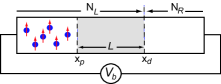
Figure 1: (color online) Schematics of the model structure we consider. Full spin polarization, $P_{n}=1$ is assumed for $x<x_{p}$.

The nonlinear, coupled equations (1,2,3,6) need to be solved self-consistently for a given applied bias voltage, doping concentration profile, nonequilibrium spin distributions, and relaxation times. We use a numerical approach based on finite difference and relaxation methods, that we originally developed for the study of nonequilibrium effects in charge transport through ultrasmall, inhomogeneous semiconductor channels.csontosJCE ; csontosAPL As boundary conditions, we adopt the following scheme: For the potential, the values at the system boundaries are fixed to $\phi(x_{l})=V_{b}$ and $\phi(x_{r})=0$ ($l,r$ denote the left and right boundary of the sample, respectively), corresponding to an externally applied voltage $V_{b}$. The electron charge density is allowed to fluctuate in the system subject to the condition of global charge neutrality, which is enforced between each successive iteration in the self-consistent Poisson-Boltzmann loop. The spin density at the DMS boundary and in the DMS is determined by the degree of polarization $P_{n}=(n_{\uparrow}-n_{\downarrow})/(n_{\uparrow}+n_{\downarrow})$, for which the density is defined according to $n_{\uparrow(\downarrow)}=n/2(1\pm P)$. In the calculations, the size of the contacts has to be large enough, such that the electric field deep inside the contacts is constant and low. This allows us to use the analytical, linear response solution to the BTEs (1)

$$f_{\uparrow(\downarrow)}(x_{l,r},v)=f^{0}_{\uparrow(\downarrow)}(x_{l,r},v)[1-vE(x_{l,r})\tau_{m}/k_{B}T]~{},$$ (7)

as boundary conditions at $x_{l,r}$, where we use the local equilibrium distribution $f^{0}_{\uparrow(\downarrow)}(x_{l,r},v)$ and local electric field, $E(x_{l,r})$, obtained from the previous numerical solution to the Poisson-Boltzmann iterative loop. More details of the numerical procedure for a similar problem are given in Ref. csontosPHYSICAE, .

The model structure that we study is described in Fig. 1. As seen in the figure, the system is inhomogeneous with respect to both charge and spin degrees of freedom. Spin-polarized electrons, with $P_{n}=1$, are injected from a diluted magnetic semiconductor(DMS)-like portion,DMS ; fiederlingohno defined for $x<x_{p}$, into a nonmagnetic semiconductor (NMS) part. The spin-polarized electrons subsequently relax due to spin-flip scattering for $x>x_{p}$, at the rate $1/\tau_{{\mathrm{s}f}}$ (where $\tau_{\uparrow\downarrow}=\tau_{\downarrow\uparrow}=2\tau_{{\mathrm{s}f}}$), to the asymptotic unpolarized value $P_{n}=0$ for $x\gg x_{p}$. The doping concentration is defined as $N_{D}=N_{L}$ and $N_{D}=N_{R}$ for $x<x_{d}$ and $x\geq x_{d}$, respectively. The following material and system parameters have been used in our study: $T=300$ K, $m^{\ast}=0.067$m₀, $\tau_{{\mathrm{m}}}=0.1$ ps (typical for GaAs at room temperature), $\tau_{{\mathrm{s}f}}=1$ ns, $N_{L}=10^{21}$ m^-3, $V_{b}=-0.3$ V. The total system size is 5 $\mu$m, i.e., $x_{l,r}=\mp 2.5$ $\mu$m.

III Numerical results: Enhancement and suppression of spin polarization at doping interfaces

In the following, we present numerical results for a spin and charge inhomogeneous semiconductor structure and highlight the characteristics of electric field effects on the spin polarization. In Fig. 2 we study the propagation of spin-polarized electrons across two spin- and charge-inhomogeneous interfaces, separated by $L=0.2$ $\mu$m (grey mid-region), as a function of different doping concentrations $N_{R}$. In Fig. 2(a) we show the spin density imbalance, $\delta_{\uparrow\downarrow}=n_{\uparrow}-n_{\downarrow}$ (solid lines), and the total charge density, $n$ (dashed lines), for $N_{R}=rN_{L}$, where $r=1,2,5,10,20$ ($N_{L}=10^{21}$ m^-3. The lowest solid and dashed curves correspond to $\delta_{\uparrow\downarrow}$ and $n$ of a charge homogeneous sample, $N_{R}=N_{L}$, in which the electric field is accordingly constant, as shown by the thick, solid line in Fig. 2(d). In contrast to the constant total charge density (bottom dashed line), for the charge homogeneous case, the spin density imbalance, $\delta_{\uparrow\downarrow}$ (bottom solid line), decreases monotonically for $x>x_{p}$, which coincides with the position of the DMS/NMS interface and the onset of the spin flip scattering rate $1/\tau_{{\mathrm{s}f}}$. The decay is exponential and can be understood in terms of the drift-diffusion description in the YF model.yu Within this model, the spin density imbalance decay can be described by $\delta_{\uparrow\downarrow}\sim\exp[-x/L_{D(U)}]$ where

$$L_{D(U)}=\left\{-(+)\frac{\left|eE\right|}{2k_{B}T}+\sqrt{\left(\frac{eE}{2k_{B}T}\right)^{2}+\frac{1}{L_{s}^{2}}}\right\}^{-1}~{},$$ (8)

and where, $L_{d(u)}$ are electric-field dependent spin diffusion lengths, describing spin propagation antiparallel (parallel) to the electric field. In eq. (8) $L_{s}=\sqrt{D\tau_{sf}}$ is an intrinsic spin-diffusion length in the absence of an electric field and $D=k_{B}T\tau_{m}/m^{\ast}$, as obtained from the Einstein relation. From eq. (8) it follows that the spin-diffusion length is enhanced in the direction anti-parallel to an applied electric field and suppressed in the direction parallel to the field.yu Our numerical results agree with these considerations for the homogeneous system.

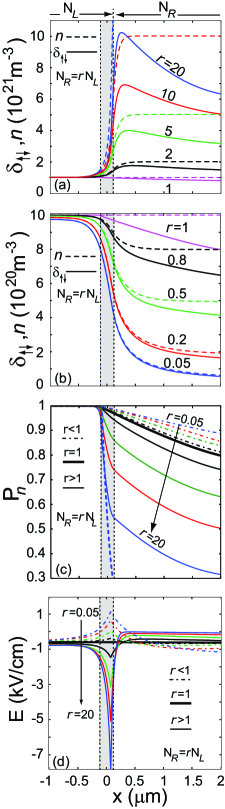
Figure 2: (color online) Spin density imbalance $\delta_{\uparrow\downarrow}$ (solid lines) and total charge density $n$ (dashed lines) for a spin and charge inhomogeneous structure as depicted in Fig. 1 for different doping concentrations (a) $N_{R}=1,2,5,10,20\cdot N_{L}$, and (b) $N_{R}=0.05,0.2,0.5,0.8,1\cdot N_{L}$ (increasing from bottom to top). (c) Spin density polarization $P_{n}$, and (d) electric field distribution for the same structure. The structure parameters are $N_{L}=10^{21}$ m^-3, $L=0.2$ $\mu$m, $\tau_{{\mathrm{s}f}}=0.5$ ns, $\tau_{{\mathrm{m}}}=0.1$ ps, $V_{b}=-0.3$ V.

For increasing $N_{R}$, the total charge density, $n$, naturally increases monotonically for $x>x_{d}$, reaching $n\approx N_{R}$ on the order of a screening length to the right of the doping interface. The spin density imbalance $\delta_{\uparrow\downarrow}$, however, has a more complicated behavior. At the interface between the two doping regions, defined at $x_{d}$, a sharp increase of $\delta_{\uparrow\downarrow}$ is observed, which subsequently peaks below the maximum value of $n$, followed by a monotonic decay. Similar spin accumulation was recently reported by Pershin and Privman.pershinPRL2003 We note and emphasize, however, that the spin accumulation peak is significantly lower than the maximum value of $n$ around the doping interface, e.g., for the $N_{R}=20\cdot 10^{21}$ m^-3 sample, $\delta_{\uparrow\downarrow}$ reaches only $\approx 50\%$ of the corresponding value in $n$.

For $N_{R}<N_{L}$, when electrons are injected from a high to a low doping region, the situation is reversed. In Fig. 2(b), the dashed and solid lines correspond to $n$ and $\delta_{\uparrow\downarrow}$, calculated for different values of $N_{R}=rN_{L}$, where $1\geq r\geq 0.05$. For decreasing $N_{R}$, $\delta_{\uparrow\downarrow}$ (and naturally $n$) decreases as well.

The observed increase (decrease) of $\delta_{\uparrow\downarrow}$ with increasing (decreasing) $N_{R}$ can at first order be understood in terms of the large difference between the intrinsic spin relaxation length, $L_{s}$, and the Debye screening length, $L_{DB}$. The screening length is generally shorter than the spin relaxation length. For example, for the range of doping concentrations considered here, we find $0.03<L_{DB}<0.6$ $\mu$m, whereas $L_{s}\approx 1.8$ $\mu$m. The spin density imbalance can be written in terms of $\delta_{\uparrow\downarrow}=n-2n_{\downarrow}$. Since $L_{s}>L_{DB}$, the total charge density, $n$, will increase (decrease) faster than $n_{\downarrow}$ with increasing (decreasing) $N_{R}$. Hence, one would expect the spatial dependence of $n$ to dominate $\delta_{\uparrow\downarrow}$ within a screening length of the doping interface. This is clearly seen by comparison between $\delta_{\uparrow\downarrow}$ (solid lines) and $n$ (dashed lines) in Figs. 2(a,b).

For $x\gg x_{d}$, $\delta_{\uparrow\downarrow}$ is seen to decrease exponentially. Furthermore, the decay rate is larger for increasing doping concentrations $N_{R}$. One can understand this spatial dependence from previous arguments and the model of YF. For $x\gg x_{d}$ the total charge density $n$ and the electric field is constant (and thus we can apply the YF model) and the spin-flip scattering drives the nonequilibrium spin density distribution exponentially toward equilibrium, $\delta_{\uparrow\downarrow}=0$ on a length scale given by eq. (8). Since an increase in $N_{R}$ gives rise to a decrease of the electric field in that region [see Fig. 2(d) for the electric profiles] the spin diffusion length correspondingly decreases consistent with the predictions of eq. (8), giving rise to a faster decay of the spin density imbalance.

The description provided by eq. (8), however, fails to describe the magnitude, as well as the spatial dependence of $\delta_{\uparrow\downarrow}$ around the doping interface. For example, considering first the curves with $N_{R}>N_{L}$, for $N_{R}=2N_{L}$, $\delta_{\uparrow\downarrow}$ follows the spatial profile of $n$ rather closely around the interface region. Surprisingly, with increasing $N_{R}$, the maximum value reached by $\delta_{\uparrow\downarrow}$ becomes increasingly smaller than $N_{R}$, and the spin density imbalance thus gets strongly suppressed. This is an unexpected finding, and in contradiction the YF model and with eq. (8), since, according to this equation, a strong built-in negativ field, such as shown in Fig. 2(d), around the doping interface should enhance the spin diffusion length significantly and hence, should yield $\delta_{\uparrow\downarrow}\approx n$ until the electric field drops again for $x>>x_{d}$.

This discrepancy is also well illustrated in the spin density polarization, $P_{n}$, shown in Fig. 2(c). Although, as naively expected, $P_{n}=\delta_{\uparrow\downarrow}/n$ drops sharply around the interface due to the sharp rise in $n$, the dependence on $N_{R}$ is in contradiction with eq. (8) due to the following: An increase in $N_{R}$, yields a sharp increase of $|E|$ around the interface [see Fig. 2(d)], and should therefore lead to a significant increase of the ”downstream” spin diffusion length, $L_{D}$, according to eq. (8). Thus, an increase in $N_{R}$ should be beneficial for $\delta_{\uparrow\downarrow}$ and $P_{n}$, in contradiction to our findings. For $N_{R}<N_{L}$, a similar unexpected dependence on $N_{R}$ is observed.

Clearly, one needs to go beyond the YF model (which is valid for a system with local charge neutrality) in order to understand spin polarized transport in the presence of inhomogeneous electric fields . As we will discuss below, the sign and magnitude of the electric field and electric field gradients around the interface are crucial for determining the magnitude and spatial dependence of the spin density imbalance and polarization around the doping interface.

IV Spin drift-diffusion equations

A qualitative understanding of the unexpected spatial dependence of $P_{n}$ and $\delta_{\uparrow\downarrow}$, can be obtained by reexamining the spin drift-diffusion equations. Previous works have mainly focused on the charge homogeneous case.yu ; osipovPRB2005 ; agrawalPRB2005 ; deryPRB2006 This is a natural assumption since the screening length is expected to be much shorter than the intrinsic spin relaxation length, leading one to assume quasi-local charge neutrality. However, as we will show below, corrections to the spin drift-diffusion equations of YFyu yield that even quasi-local deviations from charge neutrality can have a very strong impact on the spin polarization.

In the following, we perform the same steps as YFyu for the derivation of the spin drift-diffusion equations. The current for spin-up and spin-down electrons can be written as

$${\mathbf{j}}_{\uparrow(\downarrow)}=\sigma_{\uparrow(\downarrow)}{\mathbf{E}}+eD_{\uparrow(\downarrow)}\nabla n_{\uparrow(\downarrow)}~{},$$ (9)

where $D_{\uparrow(\downarrow)}$ and $\sigma_{\uparrow(\downarrow)}$ are the diffusion constants and conductivities for the spin-up(down) species. Here, the conductivities refer to $\sigma_{\uparrow(\downarrow)}=en_{\uparrow(\downarrow)}\mu_{\uparrow(\downarrow)}$, in terms of the mobilities $\mu_{\uparrow(\downarrow)}$ and densities $n_{\uparrow(\downarrow)}$ of spin-up(down) electrons. The continuity equations for the two species require that

$$\frac{\partial n_{\uparrow(\downarrow)}}{\partial t}=-\frac{n_{\uparrow(\downarrow)}}{\tau_{\uparrow\downarrow(\downarrow\uparrow)}}+\frac{n_{\downarrow(\uparrow)}}{\tau_{\downarrow\uparrow(\uparrow\downarrow)}}+\frac{1}{e}\nabla\cdot{\mathbf{j}}_{\uparrow(\downarrow)}~{},$$ (10)

where $\tau_{\uparrow\downarrow}(\tau_{\downarrow\uparrow})$ are the spin-flip scattering rates. In steady-state eqs. (9,10) result in

$$\nabla\sigma_{\uparrow(\downarrow)}\cdot{\mathbf{E}}+\sigma_{\uparrow(\downarrow)}\nabla\cdot{\mathbf{E}}+eD_{\uparrow(\downarrow)}\nabla^{2}n_{\uparrow(\downarrow)}=-\frac{en_{\uparrow(\downarrow)}}{\tau_{\uparrow\downarrow(\downarrow\uparrow)}}+\frac{en_{\downarrow(\uparrow)}}{\tau_{\downarrow\uparrow(\uparrow\downarrow)}}~{}.$$ (11)

For a NMS $\mu_{\uparrow}=\mu_{\downarrow}$, and $D_{\uparrow}=D_{\downarrow}$. Multiplying eq. (11) with $\sigma_{\downarrow}(\sigma_{\downarrow})$ and substracting them from each other we arrive to the following expression for the spin density imbalance $\delta_{\uparrow\downarrow}=n_{\uparrow}-n_{\downarrow}$

$$\nabla^{2}\delta_{\uparrow\downarrow}+\frac{e{\mathbf{E}}}{k_{B}T}\nabla\delta_{\uparrow\downarrow}+\frac{e{\mathbf{E}}}{2k_{B}T}\delta_{\uparrow\downarrow}\nabla\cdot{\mathbf{E}}-\frac{\delta_{\uparrow\downarrow}}{L_{s}}=0~{},$$ (12)

where we have used the Einstein relation $\mu=eD/k_{B}T$, $\tau_{s}$ is the spin relaxation time $\tau_{s}^{-1}=\tau_{\uparrow\downarrow}^{-1}+\tau_{\downarrow\uparrow}^{-1}$ ($\tau_{\uparrow\downarrow}=\tau_{\downarrow\uparrow}$), and $L_{s}=\sqrt{D\tau_{s}}$ is the intrinsic spin diffusion length.

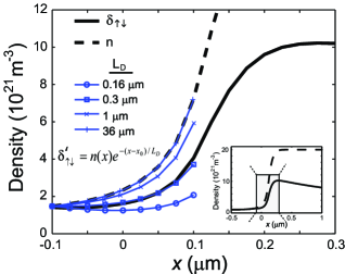
Figure 3: (color online) Total charge density (dashed line) and spin density imbalance (solid line) profiles calculated for $N_{R}=20N_{L}$. Additional curves for $-0.1<x<0.1$ $\mu$m correspond to $\delta_{\uparrow\downarrow}=n(x)\exp[-(x+0.1)/L_{D}]$ for $L_{D}=0.16,0.3,1,36$ $\mu$m, as described in the text. Inset shows $n$ and $\delta_{\uparrow\downarrow}$ for a larger region.

Equation (12) is a drift-diffusion equation for the spin density imbalance $\delta_{\uparrow\downarrow}$ and contains terms depending on both the electric field, and the electric field gradient. We note that in fact eq. (12) resembles the corresponding equations in Refs. yu, , but with an additional term proportional to $\nabla\cdot{\mathbf{E}}$. Similarly to Refs. yu, we can use the roots of the characteristic equation for eq. (12) to define up- and down-stream spin diffusion lengths from eq. (12) leading up to the following equation

$$L_{D(U)}^{\prime}=\left[-(+)\frac{|eE|}{2k_{B}T}+\sqrt{\left(\frac{eE}{2k_{B}T}\right)^{2}+\frac{1}{L_{s}^{2}}-\frac{e\nabla E}{k_{B}T}}\right]^{-1}~{}.$$ (13)

Notice that eq. (13) is only defined ”locally”, over a region where $\nabla\cdot{\mathbf{E}}$ can be considered constant, and where an average value of the electric field is used. Note also that the above equations are also valid for ferromagnetic semiconductors provided the mobility and diffusion constant are replaced with the ones corresponding to the minority-spin species.yu ; flattePRL

A comparison between eqs. (13) and (8) shows that eq. (13) contains an additional term $-e\nabla E/k_{B}T$ in the square root expression. This term is a correction to the YF model which describes the important role that inhomogeneous electric fields can play on spin polarized transport.

V Discussion

From eq. (13) it is thus seen that the drift-diffusion length depends strongly on the gradient of the electric field; Consequently, the spin density imbalance and polarization decay lengths are enhanced or suppressed based not only on the sign of the electric field alone.yu On the contrary, depending on the profile of the electric field, the gradient term in eq. (13) can either enhance or suppress the spin-polarization propagation significantly, as seen explicitly in our calculated results in Fig. 2(a-c).

To illustrate the dramatic impact of the electric field gradient term on the spin polarization diffusion, we calculate $L^{\prime}_{D(U)}$ for the central region of the structure, $x_{p}<x<x_{d}$. Using a linear approximation of the electric field within this region, for the structure with $N_{R}=20\cdot 10^{21}$ m^-3 [bottom, solid line in Fig. 2(c)], the intrinsic spin-diffusion length $L_{s}\approx 1.8$ $\mu$m, and an electric field value taken at mid-channel, $E=-2.9$ kV/cm, eq. (13) yields $L^{\prime}_{D}\approx 0.16$ $\mu$m and $L^{\prime}_{U}\approx 0.06$ $\mu$m. In comparison, an evaluation of eq. (8) using the same value of the electric field, yields $L_{D}\approx 36$ $\mu$m, $L_{U}\approx 0.09$ $\mu$m. Hence, the electric field gradient in this case decreases the “local” (around the interface) spin diffusion length, along the direction of (charge) transport, by two orders of magnitude! The injected spin density polarization is thus destroyed by the inhomogeneous electric field at the doping interface.

To verify the validity of eq. (13), we compare $\exp[-(x-x_{p})/L^{\prime}_{D}]$, using $L^{\prime}_{D}=0.16$ $\mu$m as before, with the results (for $P_{n}$) from our Boltzmann-Poisson numerical calculation, within $x_{p}<x<x_{d}$. The results, plotted in Fig. 2(c) (thick dashed line for the highest $N_{R}$ value), are found to agree very well with the numerically calculated values.

We further do a similar analysis for the spin density imbalance, $\delta_{\uparrow\downarrow}$. Here, we compare the numerically calculated values for $\delta_{\uparrow\downarrow}$, and $n$ for the same doping concentration profile with $N_{R}=20N_{L}$, with $\delta^{\prime}_{\uparrow\downarrow}=n(x)\exp[-(x-x_{0})/L^{\prime}_{D}]$, using the numerically calculated values of $n(x)$, and the estimates of $L_{D}$ and $L^{\prime}_{D}$ above. The results are shown in Fig. 3 for $L^{\prime}_{D}=0.16,0.3,1$ and 36 $\mu$m, the first and latter values corresponding to the previously estimated values using eqs. 13 and 8. The numerically calculated curve of $\delta_{\uparrow\downarrow}$ is best fitted to an effective spin diffusion length of $L^{\prime}_{D}=0.3$ $\mu$m, which is in good agreement with the value obtained from eq. (13), any discrepancies being due to the approximations in the choice of $\nabla E$ and $E$ in eq. (13). Nevertheless, it is clear that the spin diffusion length around the interface is much smaller than the intrinsic one, $L_{s}$, and the corresponding $L_{D}$, obtained within the YF model, which is only valid in the (locally) charge neutral case.

Reversing the sign of the electric field gradient, the spin density polarization $P_{n}$ is in fact enhanced in comparison to the homogeneous case. This is illustrated by the dashed-dotted curves in Fig. 2(c), which correspond to $N_{R}<N_{L}$. Since the electric field gradients are not as large as for the previously studied case [see Fig. 2(d)], the corresponding increase in $P_{n}$ is more modest.

We further clarify the effects of electric field gradients on the relaxation of nonequilibrium spin distributions. Figure 4 shows the results for $\delta_{\uparrow\downarrow}$ (a), $P_{n}$ (b), and $E(x)$ (c) calculated for $N_{R}=10N_{L}=10^{22}$ m^-3 and different channel lengths, $0<L<3$ $\mu$m. We have offset all curves in space such that $x_{p}$, i.e., the position of the DMS/NMS interface, coincides. For $L=0$, $\delta_{\uparrow\downarrow}$ shows a sharp increase around the doping interface, followed by a monotonic, exponential decrease, whereas the spin density polarization, $P_{n}$, shows an exponential decrease only, with decay length similar to $\delta_{\uparrow\downarrow}$, but with values below the corresponding values for the homogeneous system (thick solid line). This is in agreement with our previous discussion and agrees with the fact that the electric field [see Fig. 4(c)] in the right-hand side region is significantly lower than for the homogeneous case [thick solid line in Fig. 4(c)].

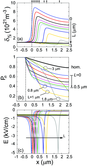
Figure 4: (color online) Spin density imbalance $\delta_{\uparrow\downarrow}$ (a), spin density polarization $P_{n}$ (b), and electric field distribution (c) for a spin and charge inhomogeneous structure as depicted in Fig. 1, for different channel lengths, $L=0,0.1,0.2,0.3,0.4,0.5,0.8,1.0,1.8,3.0$ $\mu$m. Curves are offset such that $x_{p}=0$ in all cases. Parameters are $N_{L}=10^{21}$ m^-3, $N_{R}=10^{22}$ m^-3, $\tau_{{\mathrm{s}f}}=1$ ns, $\tau_{{\mathrm{m}}}=0.1$ ps, $V_{b}=-0.3$ V. Arrows indicate the position at $x_{d}$. The thick, solid line in the figures corresponds to the charge homogeneous case.

For increasing channel lengths the spin imbalance decreases significantly. In particular, $\delta_{\uparrow\downarrow}$ for the inhomogeneous structure is smaller than the corresponding homogeneous one (thick solid line) for $x<x_{d}$ and a dip-like feature is formed for large $L$ prior to the interface between the two doping regions, where $\delta_{\uparrow\downarrow}$ is seen to increase and reach a peak. Interestingly, this also occurs for $x<x_{d}-L_{DB}$ for the structures with $L\gg L_{DB}$, i.e., in a region with very small electric field gradients [see Fig. 4(c)]. This illustrates the fact that, although the electric field gradients in this region are very small [virtually unobservable on the scale shown in Fig. 4(c)], they are large enough to yield significant influence on the spin density imbalance. In the spin density polarization, $P_{n}$, the inhomogeneous electric fields manifest as nonexponential spatial dependence, which further accentuates the importance of electric field gradients in the propagation of spin-polarized carriers.

We note that spin accumulation at the interface between regions with different doping concentrations, such as seen in Fig. 2(a), has been previously discussed by Pershin and Privman.pershinPRL2003 It was argued that injecting spin-polarized electrons across a low-to-high doping concentration interface yields a significant enhancement of the spin polarization. However, the increase is seen only for $\delta_{\uparrow\downarrow}$, i.e., the spin density imbalance, which the authors considered in their work. This is, however, only due to the overall total charge density increase as discussed above. A closer look and comparison to the total charge density, as shown in Fig. 2(a) showed that $\delta_{\uparrow\downarrow}$ is suppressed at the interface, which becomes even more evident when considering the actual spin density polarization, $P_{n}$. Moreover, we find that $P_{n}$ can be enhanced for spin-polarized electron injection across a high-to-low doping concentration interface, due to the positive electric field gradients [see dashed-dotted lines in Fig. 2(c)].

We would also like to point out the large difference between the spin density imbalance, $\delta_{\uparrow\downarrow}$, and polarization, $P_{n}$, in inhomogeneous systems. Previously in the literature, these two quantities have been used interchangeably, which certainly is true for charge homogeneous systems. For charge inhomogeneous systems on the other hand, depending on the measuring setup at hand, the correct quantity has to be studied and discussed for the optimization and assesment of spin injection, transport and detection schemes.

We again emphasize that the observed characteristics in the polarization, $P_{n}$, are quite unexpected. Naively, one would expect that, e.g., an increase in doping concentration would result in a simple decrease of $P_{n}$ (which is indeed observed), due to the rapid increase in the total charge density, $n$. However, it is not obvious how $P_{n}$ should vary for different doping concentrations, as in the setup discussed in our paper, and what the magnitude and spatial dependence of $P_{n}$ should be. Our numerical calculations, discussion and analysis above, clearly show that the spatial dependence of the spin density polarization is quite complicated in the presence of inhomogeneous electric fields.

VI Conclusions

The results and discussion presented in our paper predicts that, even weakly, inhomogeneous electric fields can significantly change the spin diffusion length. Hence, purely electrical effects may have a profound impact on spin injection, spin transport, and spin detection, three key ingredients for the realization of semiconductor spintronics. Our findings should be relevant to current experimental efforts, as well as theoretical studies in the field, where we have shown that it is crucial to take into account inhomogeneous electric fields self-consistently, in particular around doping interfaces as discussed in our paper.

- (1) H. Munekata, H. Ohno, S. von Molnar, A. Segmüller, L.L. Chang, and L. Esaki, Phys. Rev. Lett. 63, 1849 (1989); H. Ohno, Science 281, 951 (1998), and references therein.
- (2) R. Fiederling, M. Keim, G. Reuscher, W. Ossau, G. Schmidt, A. Waag, L.W. Molenkamp, Nature 402, 787 (1999); Y. Ohno, D.K. Young, B. Beschoten, F. Matsukura, H. Ohno, and D.D. Awschalom, Nature 402, 790 (1999).
- (3) Z. G. Yu, and M. E. Flatté, Phys. Rev. B 66, 201202(R) 2002; Z. G. Yu, and M. E. Flatté, ibid. 66, 235302 (2002).
- (4) S. A. Crooker, and D. L. Smith, Phys. Rev. Lett. 94, 236601 (2005).
- (5) G. Schmidt, C. Gould, P. Grabs, A.M. Lunde, G. Richter, A. Slobodskyy, and L.W. Molenkamp, Phys. Rev. Lett. 92, 226602 (2004).
- (6) P. Van Dorpe, Z. Liu, W. van Roy, V.F. Motsnyi, M. Sawicki, G. Borghs, and J. De Boeck, Appl. Phys. Lett. 84, 3495 (2004).
- (7) M. Kohda, Y. Ohno, F. Matsukura, and H. Ohno, Physica E 32, 438 (2006).
- (8) C. Adelmann, J.Q. Xie, C.J. Palmstrøm, J. Strand, X. Lou, J. Wang, and P.A. Crowell, J. Vac. Sci. Technol. 23, 1747 (2005).
- (9) Y. Y. Wang, and M. W. Wu, Phys. Rev. B 72, 153 301 (2005).
- (10) E. Ya. Sherman, Appl. Phys. Lett. 82, 209 (2003).
- (11) D. Csontos, and S. E. Ulloa, J. Comp. Electronics 3, 215 (2004).
- (12) D. Csontos, and S. E. Ulloa, Appl. Phys. Lett. 86, 253103 (2005).
- (13) D. Csontos, and S. E. Ulloa, Physica E 32, 412 (2006).
- (14) Y. V. Pershin, and V. Privman, Phys. Rev. Lett. 90, 256602 (2003).
- (15) S. Agrawal, M.B.A. Jalil, S.G. Tan, K.L. Teo, and T. Liew, Phys. Rev. B 72, 075352 (2005).
- (16) V. V. Osipov, and A. M. Bratkovsky, Phys. Rev. B 72, 115322 (2005).
- (17) H. Dery, Ł. Cywiński, and L.J. Sham, Phys. Rev. B 73, 041306(R) (2006).
- (18) M. E. Flatté, and J. M. Byers, Phys. Rev. Lett. 84, 4220 (2000).