Condition numbers and scale free graphs

Abstract

In this work we study the condition number of the least square matrix corresponding to scale free networks. We compute a theoretical lower bound of the condition number which proves that they are ill conditioned. Also, we analyze several matrices from networks generated with the linear preferential attachment model showing that it is very difficult to compute the power law exponent by the least square method due to the severe lost of accuracy expected from the corresponding condition numbers.

I Introduction

In the last years several networks were analyzed, like internet routers, biological and metabolic networks, or sexual contacts FFF , JTAOB , LEASA , and the node degree distributions of all of them seem to follow a power law. Also, several models of graph growth were presented in order to explain the emergence of this power law distribution AB , KR , DMS . However, several critics appeared, mainly focusing on sampling bias ACKM , LKJ , PR , CCG , CM , AAB , LBCX , and the quality of data fitting HJ , KW , SMA .

Recently, a simple experiment was presented in GMY studying the linear fit on the log log scale of computationally generated data with a pure power law distribution, and a severe bias error was reported ($36\%$, and $29\%$ with logarithmic bins).

In this work we present an underlying problem which explains those errors: regrettably, the matrix in the least square method is ill conditioned. Let $n$ be the maximum degree of the network, we show that the condition number grows at least as the logarithm of $n$. Moreover, we introduce a parameter $c\in[0,1]$ and we consider only the node degree distribution on $[cn,n]$ (in fact, this is a usual procedure, see N ). Numerical computations show that the situation is worse when we focus on the tail of the distribution.

Our results complement the ones in KW , where biological networks were considered and a different statistical problem arose, since on that work the power law fit was performed with the maximum likelihood method.

Also, we compute the matrix condition for scale free graphs generated with the linear preferential attachment model introduced by Barabasi and Albert AB . We show that the matrix condition grows when the network size increases.

II Main Results

II.1 Condition Number

For a given matrix $A\in R^{m\times m}$, and a matrix norm $\|.\|$, the condition number is defined as

$$cond(A)=\|A\|\|A^{-1}\|,\qquad cond(A)=\infty\,\mbox{ if }\,det(a)=0$$

Usually, for the $2$-norm the condition is denoted $cond(A)_{2}$. The $2$-norm is an operator type norm, i.e. for $v\in R^{m}$, taking the vectorial Euclidean norm

$$\|v\|_{2}:=\left(\sum_{i=1}^{m}|v_{i}|^{2}\right)^{\frac{1}{2}}$$

we have

$$\|A\|_{2}=sup\{\|Av\|_{2}\ \ :\ \ \|v\|_{2}=1\}.$$

Concerning the condition number, the following results are well known GV :

$$cond(A)_{2}=\frac{\lambda_{max}}{\lambda_{min}}.$$ (1)

where $\lambda_{min}$ and $\lambda_{max}$ are the minimum and the maximum eigenvalue (in absolute value), and

$$\frac{1}{cond(A)_{2}}=inf\left\{\frac{\|A-S\|_{2}}{\|A\|_{2}}\ :\ S\ \ \mbox{singular}\right\}$$ (2)

which says that $cond(A)_{2}$ is the reciprocal of the relative distance of $A$ to the set of singular matrices.

The interest in the condition number for matrices is related to the accuracy of computations, since it gives a bound for the propagation of the relative error in the data when a linear system is solved. If $cond(A)\sim 10^{k}$, then $k$ is roughly the number of significant figures we can expect to lose in computations.

More precisely, for a general system $Ax=b$, if we consider a perturbation on the right hand side $\tilde{b}$, then calling $\tilde{x}$ to the exact solution of $A\tilde{x}=\tilde{b}$ it can be shown that

$$\frac{\|x-\tilde{x}\|_{2}}{\|x\|_{2}}\leq cond(A)_{2}\frac{\|b-\tilde{b}\|_{2}}{\|b\|_{2}}.$$

A practical rule in statistics is to avoid the least square method when the condition number is greater than or equal to $900$ (indeed they define $\kappa(A)=cond(A)^{1/2}$, and $\kappa\geq 15$ is a strong sign of collinearity, see for example CHP ).

II.2 Theoretical Results

Let us consider a graph $G$ with $k$ nodes $x_{1},\cdots,x_{k}$, and $d(x_{i})$ is the degree of node $x_{i}$, that is, the number of links emanating from $x_{i}$. Let us define

$$n=max\{d(x_{i})\,:\,1\leq i\leq k\}.$$

For each $j$, $1\leq j\leq n$, let $h_{j}$ be the number of nodes with degree $j$. The existence of a power law dependence $h(d)=ad^{\gamma}$ is usually observed in a log-log plot, and computed with the least square method after a logarithmic change of variables.

First we assume that the degrees span the full integer interval $[1,n]$. In this case the matrix $A_{n}$ corresponding to the least square fit, regardless of the measured data, is given by

$$A_{n}=\left(\begin{array}[]{cc}n&\sum_{j=1}^{n}\ln(j)\\ \sum_{j=1}^{n}\ln(j)&\sum_{j=1}^{n}\ln^{2}(j)\\ \end{array}\right)$$

In certain a sense, this correspond to the best situation where the data span the full range of variables. The following result estimates the condition number of $A_{n}$, when $n\to\infty$:

Theorem II.1

For $n$ large, it holds

$$cond(A_{n})_{2}\sim\ln^{4}(n)$$

Proof: We use here (1). A straightforward computation of the eigenvalues of $A_{n}$ gives

$$\lambda_{max}=\Big{(}n+\sum_{j=1}^{n}\ln^{2}(j)\Big{)}+\sqrt{\Delta}$$ (3)

$$\lambda_{min}=\Big{(}n+\sum_{j=1}^{n}\ln^{2}(j)\Big{)}-\sqrt{\Delta},$$ (4)

where

$$\Delta=\Big{(}n-\sum_{j=1}^{n}\ln^{2}(j)\Big{)}^{2}+4\Big{(}\sum_{j=1}^{n}\ln(j)\Big{)}^{2}.$$

For $n$ large we can write

$$\sum_{j=1}^{n}\ln(j)\sim n(ln(n)-1))+O(ln(n))$$

and

$$\sum_{j=1}^{n}\ln^{2}(j)\sim n(ln^{2}(n)-2ln(n)+2)+O(ln^{2}(n)).$$

Replacing this expressions in (3) and (4), we get by taking limit

$$lim_{n\to\infty}\frac{\frac{\lambda_{max}}{\lambda_{min}}}{ln^{4}(n)}=1$$

$\hfill\Box$

Since in practice logarithmic bin is preferred (see for example N ), due to the sparsity of measurements at the tail of the distribution, our next result shows that also the corresponding matrix is ill conditioned. We suppose that the selected degrees for the computation are of the form $e^{j}$ with $1\leq j\leq n$. Calling $A_{e^{n}}$ the corresponding least square matrix, we can write

$$A_{e^{n}}=\left(\begin{array}[]{cc}n&\sum_{j=1}^{n}j\\ \sum_{j=1}^{n}j&\sum_{j=1}^{n}j^{2}\\ \end{array}\right)=\left(\begin{array}[]{cc}n&\frac{n(n+1)}{2}\\ \frac{n(n+1)}{2}&\frac{n(n+1)(2n+1)}{6}\\ \end{array}\right).$$

And the following holds

Theorem II.2

For $n$ large

$$cond(A_{e^{n}})_{2}\sim\frac{4}{3}n^{2}.$$

Proof: Using again (1), and computing explicitly the eigenvalues of $A_{e^{n}}$, we have

$$\frac{\lambda_{max}}{\lambda_{min}}=\frac{7+2n^{2}+3n+\sqrt{61+25n^{2}+42n+4n^{4}+12n^{3}}}{7+2n^{2}+3n-\sqrt{61+25n^{2}+42n+4n^{4}+12n^{3}}}$$

Hence, for $n$ large

$$cond(A_{e^{n}})_{2}=\frac{\lambda_{max}}{\lambda_{min}}\sim\frac{4}{3}n^{2}.$$

$\hfill\Box$

Numerical experiments in the next section suggest that considering a logarithmic bin of the form $ae^{j}$ is unnecessary, since the condition number grows almost independently of $a$, see Table 1.

II.3 Numerical Simulations

In this section we present several numerical computations of matrix conditions.

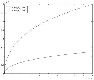
We computed the condition number of matrix $A_{n}$ numerically by using MATLAB. Also, we computed the condition number for the truncated matrix $A_{n}$, for each $n$ we consider the matrix obtained with degree values between $cn$ and $n$. The results are shown in Figure 1 for $n\leq 100000$, $c=0$ and $c=0.1$.

Figure 1: Condition number of $A_{n}$ with $n\leq 10^{5}$

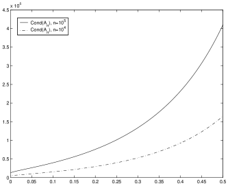
We show the dependence on $c$ in Figure 2, for $n=10^{4}$ and $n=10^{5}$, with $c$ from $0$ to $0.5$.

Figure 2: Condition number of $A_{n}$ with $0\leq c\leq 0.5$

In Table 1 we show the condition numbers for logarithmic bins of the form $ae^{j}$, $1\leq j\leq n$, for $n=10^{3},10^{4},10^{5},$ and $10^{6}$; and $a=0.1$, $a=1$ and $a=2$.

Table 1: Condition number with logarithmic bins

$ae^{j}$, $1\leq j\leq n$	a=1	a=0.1	a=2
$n=10^{3}$	$1.319\times 10^{6}$	$1.337\times 10^{6}$	$1.343\times 10^{6}$
$n=10^{4}$	$1.332\times 10^{8}$	$1.334\times 10^{8}$	$1.334\times 10^{8}$
$n=10^{5}$	$1.333\times 10^{10}$	$1.333\times 10^{10}$	$1.333\times 10^{10}$
$n=10^{6}$	$1.333\times 10^{12}$	$1.333\times 10^{12}$	$1.333\times 10^{12}$

Finally, we consider the Linear Preferential Attachment model of Barabasi and Albert. This is a model of network growth, where a new node is added with a link to a previously added node, chosen at random with a probability proportional to its degree.

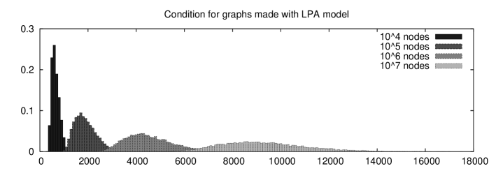
We generated $5\times 10^{4}$ graphs of $10^{4}$ nodes, $25\times 10^{3}$ graphs of $10^{5}$ nodes, $10^{4}$ graphs of $10^{6}$ nodes, and $10^{4}$ graphs of $10^{7}$ nodes, and computed the condition of the least square matrix associated with each one. We show the distribution of values of the condition number in Figure 3. Also, in Table 2 we present the computation of mean values of the condition number for $c=0$, $c=0.05$ and $c=0.1$.

Figure 3: Condition number of graphs of $10^{4}$, $10^{5}$, $10^{6}$ and $10^{7}$ nodes, computed over $5\times 10^{4}$, $2.5\times 10^{4}$, $10^{4}$ and $10^{4}$ graphs

Table 2: Mean value of condition numbers for LPA graphs with different values of $c$

Nodes	Graphs	c=0	c=0.05	c=0.1
$10^{4}$	$5\times 10^{4}$	$113.7$	$379.7$	$703.7$
$10^{5}$	$2.5\times 10^{4}$	$223.5$	$1058.4$	$1928.8$
$10^{6}$	$10^{4}$	$409.0$	$2648.5$	$4560.0$
$10^{7}$	$10^{4}$	$703.8$	$5897.6$	$9369.5$

III Conclusions

We have studied the condition number of the least square matrix corresponding to scale free networks. We computed theoretical lower bounds of the condition numbers showing that it behaves roughly as the logarithm of the maximum degree of the network, and numerical simulations support this fact. We also showed that neglecting the less connected nodes of the network (a usual practice in fact, since the interest is on the tail) things become even worse. Similar conclusions can be drawn for the logarithmic bin.

Finally, for random networks generated with the Linear Preference Attachment model, numerical computations of the condition numbers showed a severe ill condition of the least square matrices, even for small sized networks ($10^{4}$ nodes). Clearly, in this context it is very difficult to compute the power law exponent by the least square method due to the lost of accuracy expected from the corresponding condition numbers.

References

- (1) M. Faloutsos, P. Faloutsos and C. Faloutsos, Computer Communication Review, 29, (1999) 251.
- (2) H. Jeong, B. Tombor, B. Albert, Z.N. Oltvai and A.L. Barabasi, Nature, 407, (2000) 651.
- (3) F. Liljeros, C.R. Edling, L.A.N. Amaral, H.E. Stanley, and Y. Aberg, Nature 411, (2001) 907.
- (4) A-L. Barabási and R. Albert, Science, 286, (1999) 509.
- (5) P. L. Krapivsky and S. Redner, Phys. Rev. E 63, (2001) 066123.
- (6) S.N. Dorogovtsev, J.F.F. Mendes, and A.N. Samukhin, Phys. Rev. E 63, (2001) 062101.
- (7) D. Achlioptas, A. Clauset, D. Kempe and C. Moore On the Bias of Traceroute Sampling; or, Power-law Degree Distributions in Regular Graphs Proc. STOC (2005).
- (8) S. H. Lee, P-J. Kim and H. Jeong, Phys. Rev. E, to appear (cond-mat/0505232)
- (9) T. Petermann and P. De Los Rios, European Physical Journal B 38, (2004) 201.
- (10) Q. Chen, H. Chang, R. Govindan, S. Jamin, S.J. Shenker and W. Willinger, The Origin of Power Laws in Internet Topologies Revisited, Proc. of IEEE Infocom (2002).
- (11) A. Clauset and C. Moore Physical Review Letters 94, (2005) 18701.
- (12) L. Dall’Asta, I. Alvarez-Hamelin, A. Barrat, A. Vazquez and A. Vespignani, Phys. Rev. E 71, (2005) 036135.
- (13) A. Lakhina, J. Byers, M. Crovella and P. Xie Sampling Biases in IP Topology Measurements Proc. of IEEE INFOCOM ’03 (2003).
- (14) M.S. Handcock and J.H. Jones, Sexual contacts and epidemic thresholds Nature, 423, (2003) 605.
- (15) R. Khanin and E. Wit, How scale-free are biological networks? Journal of Computational Biology, to appear.
- (16) D.B. Stouffer, R.D. Malmgren and L.A.N. Amaral, Comment on Barabasi, Nature 435, 207 (2005), (2005) (physics/0510216).
- (17) M.L. Goldstein, S.A. Morris and G.G. Yen, Eur. Phys. J. B 41 (2004) 255.
- (18) M. E. J. Newman, Contemporary Physics 46, (2005) 323.
- (19) G.H. Golub and C.F. Van Loan, Matrix Computations, Johns Hopkins series in the mathematical sciences. The Johns Hopkins University Press, Baltimore and London, 3rd edition, 1996.
- (20) S. Chatterjee, A.S. Hadi, and B. Price Regression Analysis by Example, 3rd Edition, Wiley Series in Probability and Statistics (1991).