Multifractal distribution of spike intervals for two neurons with unreliable synapses

Abstract

Two neurons coupled by unreliable synapses are modeled by leaky integrate-and-fire neurons and stochastic on-off synapses. The dynamics is mapped to an iterated function system. Numerical calculations yield a multifractal distribution of interspike intervals. The Haussdorf, entropy and correlation dimensions are calculated as a function of synaptic strength and transmission probability.

Neurons communicate via synaptic contacts. When a neuron fires it sends an electric pulse (spike) along its axon. This spike activates biochemical processes in the vicinity of a synaptic contact which change the electrical membrane potential at the neighboring neuron. However, experiments on synaptic contacts show that this complex biophysical and biochemical process is not deterministic. Any incoming electrical pulse activates the synapse with some probability, only. In the cortex, transmission probabilities between 10% and 90% are reported Abeles (1991); Allen and Stevens (1994). Although model calculations show that stochastic synapses can transmit information Fuhrmann et al. (2002) it is still an unsolved mystery how a neural network with unreliable synapses is able to perform reliable computations.

A quantitative measure of the activity of neurons is the distribution of interspike intervals. Typically, one observes broad distributions which may be described by a simple mathematical approach: Each neuron is modeled by a stochastic process which is driven by random uncorrelated synaptic inputs. Hence, usually the effect of unreliable synapses is modeled by external uncorrelated noise Tuckwell (1988); Gerstner and Kistler (2002).

In this paper we investigate the dynamics of two neurons coupled by unreliable synapses. The synapses are explicitly modeled by a Bernoulli process: Any synapse transmits the spike with some probability $p$ which is independent of the state of the system. Our approach allows to calculate the spike intervals from an iterated-function-system (IFS). Our main result is a multifractal distribution of interspike intervals. The Haussdorf, entropy and correlation dimensions are calculated as a function of the synaptic strength and the probability of synaptic transmission. We find a transition between connected and multifractal support of the distribution of spike intervals.

In fact, fractal time series of neural spikes which are observed in many different biological systems have been related to quantal neurotransmitter release Lowen et al. (1997). Our model shows that even a simple on-off synapse leads to fractal structures of the neural activity. However, our simple model makes predictions for the distribution of spike intervals of two coupled neurons but it does not explain the nature of fractal time series.

The two neurons are modeled by a leaky integrate-and-fire mechanism working above threshold. In a more general framework, our model is a system of two identical pulse-coupled oscillators Mirollo and Strogatz (1990). Without synaptic contacts the neurons are deterministic and oscillate periodically, one obtains two intervals between the firing times of the two neurons. With reliable inhibitory synaptic contact, and without any delay of the synaptic transmission, the two neurons relax into a state of anti-phase oscillations with a single spike interval. With unreliable synapses, however, the system has a broad distribution of spike intervals which becomes multifractal in some range of the model parameters.

Each neuron is described by the following differential equation for the time-dependent membrane potential $V(t)$:

$$\tau\frac{dV}{dt}=\mu-V(t)$$ (1)

As soon as the potential crosses a threshold value $\theta$ it is reset to a value $V_{r}<\theta$. In addition it fires, i.e. it sends a spike to its neighbor which is transmitted with a probability $p$. If a spike is transmitted it reduces the potential of the receiving neuron by an amount $J$. For simplicity, we consider only inhibitory synapses to avoid an introduction of a refractory time. However, we believe that our main results do not depend on the details of the model.

The neurons are working above threshold, $\theta<\mu$, otherwise they would not fire at all. Hence the parameter $\mu$ controls the effect of any mechanism which forces the neurons to fire. Without synaptic couplings each neuron fires periodically with the period

$$T=\tau\,\ln\frac{\mu-V_{r}}{\mu-\theta}$$ (2)

Without loss of generality we set $V_{r}=0$, $\mu=1$ and $\tau=1$, and in the following we use the parameter $\theta=0.95$ which gives a period of $T\simeq 2.996\,\tau$.

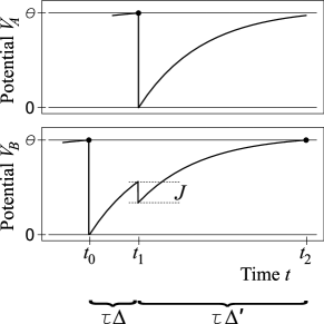
Figure 1: Membrane potential of the two neurons. The spike of neuron A at time $t_{1}$ is transmitted to neuron B.

Figure 1 shows the potential of the two neurons for a typical situation. At time $t_{1}$ the neuron A fires and the spike is transmitted to neuron B resulting in a decrease of the potential by an amount $J$. The next firing event occurs at time $t_{2}$. The time interval between firing events is denoted by $\Delta$. Using the analytic solution of the differential equation (1) one obtains an iteration of the spike intervals $\Delta$. For the quantity $x=\exp(-\Delta)$ the iteration has the form

$$x^{\prime}=f_{i}(x),\quad i\in\{1,2,3,4,5\}$$ (3)

where the five functions $f_{i}$ are selected according to the transmission probability $p$ and the previous value of $x$. For the situation of Fig. 1, which occurs with probability $p$ (transmission), one finds

$$x^{\prime}=\frac{1-\theta}{x+J}:=f_{1}(x)$$ (4)

With probability $1-p$ (no transmission) the sum $\Delta+\Delta^{\prime}=T$ is identical to the period of unperturbed oscillations which gives

$$x^{\prime}=\frac{1-\theta}{x}:=f_{2}(x)$$ (5)

Hence, two simple functions are iterated according to probability $p$ of synaptic transmission. The situation becomes slightly more complicated when neuron A overtakes neuron B, i.e. when one neuron fires twice before the other one is firing again. This occurs when the potential $V_{B}(t_{1}+)$ becomes negative after neuron A has fired, that is when $x>1-J$. In this case one has $\Delta^{\prime}=T$ or

$$x^{\prime}=1-\theta:=f_{3}(x)$$ (6)

But now $\Delta^{\prime\prime}$ depends on $\Delta$ and one finds with probability $p$

$$x^{\prime\prime}=\frac{1}{x+J+\frac{J}{1-\theta}}:=f_{4}(x)$$ (7)

and with probability $1-p$

$$x^{\prime\prime}=\frac{1}{x+J}:=f_{5}(x)$$ (8)

If the synaptic pulse $J$ is larger than $\theta/(2-\theta)$ the same neuron can even fire more than twice in a row, but we do not consider such large unphysiological values of $J$.

(a)  $J=0.1$

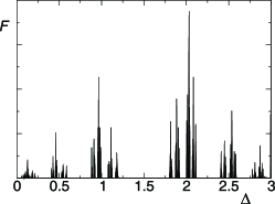
(b)  $J=0.25$

Figure 2: Histogram of the spike intervals for the transmission probability $p=0.5$ and the strength of the synaptic pulse $J=0.1$ (a) and $J=0.25$ (b).

In summary, only five simple functions are iterated to calculate the distribution of spike intervals $\Delta$. It is well known that such a system (IFS) may lead to a fractal structure of the set of iterated values Barnsley (1989). In our numerical simulations of equations (4) to (8) we have generated about $10^{11}$ spike intervals for each set of parameters. Figure 2 shows two histograms of the spike intervals for small and large values of $J$. Obviously, the distribution of spike intervals has a complex structure which we quantify by the Rényi dimensions Beck and Schlögl (1993)

$$D(\beta)=\lim_{\varepsilon\to 0}\frac{1}{\ln\varepsilon}I(\beta),\quad I(\beta)=\frac{1}{\beta-1}\ln\sum_{i=1}^{r}{p_{i}}^{\beta}$$ (9)

Here $\varepsilon$ is the size of the boxes of the histogram and $p_{i}$ is the normalized number of data points in the box $i$. The sum runs over all nonempty boxes. For $\beta=1$, the entropy $I(1)=\sum_{i=1}^{r}p_{i}\ln p_{i}$ is calculated.

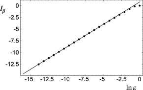
Figure 3: The quantity $I_{\beta}$ as a function of the size $\varepsilon$ of the covering boxes (here for $\beta=1$, $p=0.5$ and $J=0.15$). The slope of the figure is an estimate of the Rényi dimensions $D(\beta)$ which are shown in Fig. 4.

We consider three Rényi dimensions: The covering or box dimension $D(0)$ which is usually identical to the Haussdorf dimension, the entropy dimension $D(1)$ and the correlation dimension $D(2)$. Figure 3 shows that a plot of $I(\beta)$ versus $\ln\varepsilon$ yields a straight line over several orders of magnitude, hence the corresponding dimension can reliably be estimated from the slope of this line. In addition, we checked our results for the correlation dimension by applying the software package TISEAN to our data Kantz and Schreiber (1997).

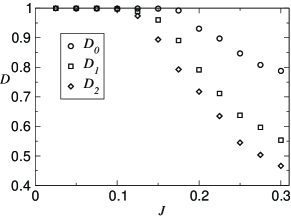
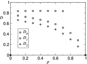
Figure 4: Rényi dimensions (a) as a function of the strength $J$ of the synaptic pulse (for $p=0.5$) and (b) as a function of the transmission probability $p$ (for $J=0.25$)

The results for the three different Rényi dimensions are shown in Fig. 4. Of course, our results obey the exact relations $D(2)\leq D(1)\leq D(0)$. With increasing coupling strength $J$ and transmission probability $p$ the three dimensions decrease. For small values of $J$ the distribution of spike intervals is smooth, hence one observes $D(0)\simeq D(1)\simeq D(2)\simeq 1$. For large values of $J$ the three dimensions are different, which means that the distribution of spike intervals is multifractal Beck and Schlögl (1993). While the covering dimension D(0), i.e. the structure of the support of the distribution, is insensitive to the value of $p$, the entropy as well as the correlation dimension decrease to the value zero in the deterministic limit $p\to 1$. In fact, for $p=1$, the distribution of spike intervals is a delta-peak at the fixed point of $f_{1}$ which gives $\Delta=-\ln(-J+\sqrt{4+J^{2}-4\theta})/2$. Surprisingly, even for $p<1$ the distribution has its maximum at this value, a sharp peak, as can be seen from Fig. 2.

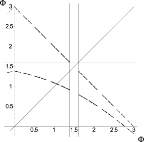
Figure 5: The phases $\phi$ of the neurons are iterated by the two functions $F_{1}$ (bottom) and $F_{2}$ (top) shown by the dashed lines. The openings of the two functions show the empty intervals in the distribution of iterated phases.

The results of Fig. 4(a) do not rule out a sharp transition between a smooth and multifractal distribution of spike intervals. In fact, for the covering dimension $D(0)$, the transition point can be found analytically. It is convenient to transform Eq. (1) to $d\phi/dt=1$ where the phase $\phi$ is defined as

$$\phi(V)=-\ln(1-V)$$ (10)

Now we consider the phase which one neuron occupies after the other one has fired. After the neuron A has fired it has the phase $\phi=0$, whereas the other neuron B has a nonzero phase $\phi_{i}$. If $\phi_{i}$ is positive it will be neuron B which fires next, namely after the time $T-\phi_{i}$. However, if $\phi_{i}$ is negative then neuron A will fire again after the time $T$. Regardless of which neuron fires, in both cases we record the phase $\phi_{i+1}$ of the neuron which has not fired. Given a phase $\phi_{i}$, the next phase $\phi_{i+1}$ results by applying one of two mappings depending on whether a spike has been transmitted at time $t_{i+1}$ or not. These two mappings $\phi_{i+1}=F_{1}(\phi_{i})$ and $\phi_{i+1}=F_{2}(\phi_{i})$ which describe the transformation of phases are as follows (see Fig. 5):

$$F_{1}(\phi) = -\ln[\exp(|\phi|-T)+J]~{}\mathrm{(transmission)}$$ (11)

$$F_{2}(\phi) = T-|\phi|~{}\mathrm{(no\;transmission)}$$ (12)

The function $F_{2}$ just flips the lower interval $[0,T/2]$ to the upper one $[T/2,T]$. The function $F_{1}$ maps the complete interval $[0,T]$ to the interval $[-\ln(1+J),-\ln(1-\theta+J)]$. If the maximum of $F_{1}$ is smaller than $T/2$, then there exists an interval in the vicinity of $T/2$ which cannot be reached from outside. In Fig. 5 this interval is indicated by the small square in the center of the figure. This interval in the center is either flipped by $F_{2}$ or mapped to an interval outside of it by $F_{1}$. This means that finally any point inside the square will leave it. In addition, no other point can enter this interval. Hence the distribution of phases has an opening on this interval. By consecutive iterations of $F_{1}$ and $F_{2}$ this opening is distributed on the complete range of phases, as depicted in Fig. 5 by the openings in the functions $F_{1}$ and $F_{2}$. This indicates – but does not prove it – that the support of the distribution of spike intervals has a fractal structure, leading to $D(0)<1$. By these arguments the support of the distribution has a fractal structure if the maximum of $F_{1}$ is smaller than $T/2$ which gives a critical point

$$J_{*}=\sqrt{1-\theta}-(1-\theta)$$ (13)

For $J<J_{*}$ the distribution fills the complete range of $\phi$ values, while for large values of $J$ the distribution has empty intervals. Indeed, this value is consistent with the data of Fig. 4(a) where the covering dimension $D(0)$ deviates from the value $D(0)=1$ at about $J_{*}=0.1736$. Note, however, that even below $J_{*}$ the distribution is multifractal because the values of $D(1)$ and $D(2)$ are still smaller than one. We do not know whether there is a sharp transition to a smooth structure for small $J$ values or whether the fractal dimensions $D(1)$ and $D(2)$ just come very close to the value one. The data of Fig. 4 do not allow to distinguish between these two possibilities.

Our system of two identical pulse-coupled oscillators with random on-off synapses is very simplified model of two coupled neurons. For instance, synaptic transmission may be multi-valued Montgomery and Madison (2004); Abarbanel et al. (2005) and time-delayed Ernst et al. (1995), and a much better model would include the dynamics of ion channels Lowen et al. (1999). However, in any model a random uncorrelated process which opens and closes synaptic transmission always yields an iterated function system which produces fractal distributions of spike intervals depending on the model parameters. Up to now, a fractal structure of spike intervals has not yet been observed. But, to our knowlege, experiments on two interacting neurons under controlled conditions have not yet been reported, either. Our model makes predictions for such an experiment which may help to clarify the stochastic nature of synaptic transmission.