Lattice Boltzmann versus Molecular Dynamics simulation of nano–hydrodynamic flows

Abstract

A fluid flow in a simple dense liquid, passing an obstacle in a two–dimensional thin film geometry, is simulated by Molecular Dynamics (MD) computer simulation and compared to results of Lattice Boltzmann (LB) simulations. By the appropriate mapping of length and time units from LB to MD, the velocity field as obtained from MD is quantitatively reproduced by LB. The implications of this finding for prospective LB-MD multiscale applications are discussed.

Micro and nano–hydrodynamic flows are playing an increasing role for many applications in material science, chemistry, and biology MICRO . To date, the leading tool for the numerical investigation of nano and micro–hydrodynamic flows is provided by molecular dynamics (MD) simulations MD . In principle, MD yields a correct description of fluids on microscopic and hydrodynamic scales. But typical length and time scales that can be covered by MD simulations of dense liquids are of the order of a few tens of nanometers and about a few hundred nanoseconds, respectively. As a result, the quest for cheaper — and yet physically realistic alternatives — is a relentless one. Mesoscopic models, and notably those arising from kinetic theory, are natural candidates to fill this gap because they operate precisely at intermediate scales between the atomistic and continuum levels. Very recently, the so–called Lattice–Boltzmann (LB) method, where a kinetic equation is solved on a lattice, has proven successful to model characteristic features of microscopic flows, such as the occurrence of slip boundary conditions near solid walls SLIPMOD .

However, whether LB is also able to reproduce complex nanoscopic flows on a quantitative level, in particular for a dense liquid, remains an open issue. Although, pioneering work of various authors has shown that hydrodynamics holds nearly down to the molecular scale in simple dense liquids (see, e.g. HYDMOL ), it is not obvious whether in the vicinity of wall–fluid or obstacle–fluid boundaries at least pair interactions on an atomistic level have to be taken into account to yield a quantitative description of fluid flows. Although LB is a particle–based method, it cannot resolve the short ranged structural order of a dense liquid since it describes a structureless lattice gas with no many–body interactions. Thus, it is not clear whether one can match the LB method with MD simulations of complex flow structures in dense liquids (e.g. coherent nanostructures).

In this paper, we aim to establish a quantitative mapping between the resolution requirements of a LB versus MD simulation of a non–trivial nano–hydrodynamic flow. Far from being a purely academic exercise, this is a primary issue to set a solid stage for future multiscale applications combining LB with atomistic methods. To this end, we have performed MD simulations of a two–dimensional Lennard–Jones fluid confined between walls that passes a thin plate–like obstacle while subject to a gravitational force field. This system is then modeled by the LB method. We demonstrate that, after the appropriate mapping of length and time units, there is a quantitative agreement between the flow fields computed with MD and LB.

First, we give a brief introduction to the LB method and the LB model used in this work. The LB method as a mesoscopic simulation tool has met with significant success in the last decade for the simulation of many complex flows LBE . We consider the LB equation in its original matrix form HSB :

$$f_{i}({\bf x}+\Delta t{\bf c}_{i},t+\Delta t)-f_{i}({\bf x},t) =$$

$$-\sum_{j}\Omega_{ij}\Delta t \!\!\!\!\!\!\!\!\!\![f_{j}({\bf x},t)-f_{j}^{\rm e}({\bf x},t)]$$ (1)

where $\Delta t$ is the time unit and $f_{i}({\bf x},t)\equiv f({\bf x},{\bf v}={\bf c}_{i},t)$, $i=0,\ldots n$, is the probability of finding a particle at lattice site ${\bf x}$ at time $t$, moving along the lattice direction defined by the discrete speed ${\bf c}_{i}$. The left–hand side of Eq. (1) represents the molecular free–streaming, whereas the right–hand side represents molecular collisions via a multiple–time relaxation towards local equilibrium $f_{i}^{\rm e}$ (a local Maxwellian expanded to second order in the fluid speed). The leading non–zero eigenvalue of the collision matrix $\Omega_{ij}$ fixes the fluid kinematic viscosity as $\nu=c_{\rm s}^{2}(1/\omega-1/2)$ (in lattice units $\Delta t=\Delta x=1$), where $c_{\rm s}$ is the sound–speed of the lattice fluid, $1/\sqrt{3}$ in the present work. In order to recover fluid dynamic behaviour at macroscopic scales, the set of discrete speeds must be chosen in such a way as to conserve mass and momentum at each lattice site. Once these conservation laws are fulfilled, the fluid density $\rho=\sum_{i}f_{i}$, and speed ${\bf u}=\sum_{i}f_{i}{\bf c}_{i}/\rho$ can be shown to evolve according to the quasi–incompressible Navier–Stokes equations of fluid–dynamics.

In the bulk flow, LB is essentially an efficient Navier-Stokes solver in disguise. The major advantages over a purely hydrodynamic description are: i) the fluid pressure is locally available site–by–site, with no need of solving a computationally demanding Poisson problem, ii) momentum diffusivity is not represented by second order spatial derivatives, but it emerges instead from the first–order LB relaxation–propagation dynamics. As a result, the time–step scales only linearly (rather than quadratically) with the mesh size, which is an important plus for down–coupling to atomistic methods, iii) highly irregular boundaries can be handled with ease because particles move along straight trajectories. This contrasts with the hydrodynamic representation, in which the fluid momentum is transported along complex space–time dependent trajectories defined by the flow velocity.

At the fluid–solid interface, we adopt the no–slip boundary condition, $\vec{u}=0$. This is imposed by the standard bounce–back procedure, i.e. by reflecting the outgoing populations back into the fluid domain along their specular direction. With reference to particles propagating south–east($\searrow$) from a north–wall boundary placed at $z=H+1/2$, the bounce-back rule simply reads as $f_{\searrow}(x,y,H+1)=f_{\nwarrow}(x+1,y,H)$ where the lattice spacing is made unity for convenience. This corresponds to a stylized two–body hard–sphere repulsion, with interaction range equal to $\sqrt{2}$ lattice units.

In this work, we use a standard nine–speed D2Q9 model LBE to simulate a two–dimensional channel flow of size $L$ and $H$ along the streamwise and cross–flow directions, respectively. At a distance $L/4$ from the inlet, a thin flat plate of height $h$ is placed, perpendicular to the direction of the main flow. The fluid is driven by a constant body force $f_{x}$ in $x$–direction which, in the absence of the vertical plate, would produce a parabolic Poiseuille profile of central speed $U=f_{x}H^{2}/(8\nu)$, $\nu$ being the kinematic viscosity of the fluid.

A similar two–dimensional channel flow of a fluid is considered in the MD simulations. As a model for the interactions between the particles, a Lennard–Jones potential is used that is truncated at its minimum and then shifted to zero. It has the following form:

$$V(r)=\left\{\begin{array}[]{ll}4\epsilon\left[\left(\frac{\sigma}{r}\right)^{12}-\left(\frac{\sigma}{r}\right)^{6}\right]+\epsilon&\mbox{for $r<2^{1/6}\sigma$}\\ 0&\mbox{otherwise,}\end{array}\right.$$ (2)

where $r$ denotes the distance between two particles. The units are chosen such that $\epsilon$, $\sigma$, the Boltzmann constant $k_{\rm B}$ and the mass of the particles $m$ are set to one. The particles are confined into a rectangular box of size $L\times H$ with $L=200\sigma$ and $H=106\sigma$. Moreover, an obstacle is placed along a line at $x=L/4$. This obstacle consists of $41$ fixed particles between $y=33.0\sigma$ and $y=73.0\sigma$ with an equidistant spacing of $1\sigma$. Thus, the obstacle has an effective width of about $1\sigma$ and a height $h=40\sigma$. For the density we chose $n=N/(LH)=0.8\sigma^{-3}$ corresponding to $N=16879$ particles in the simulation box. The equations of motions were integrated using the velocity form of the Verlet algorithm with a time step of $dt_{\rm md}=0.01\tau_{\rm md}$ with $\tau_{\rm md}\equiv\sqrt{m\sigma^{2}/(48\epsilon)}$. In order to keep the temperature constant, a Nosé–Hoover thermostat was applied binder96 .

The MD simulations were all done at temperature $T=5.3\epsilon/k_{\rm B}$. Ten independent runs were performed in order to obtain reasonable statistics. First, the systems were equilibrated for 30000 time steps. Then, walls were introduced in the system by giving all the particles at $x<3.0\sigma$ and at $x>103.0\sigma$ zero velocity. The choice of these rough walls provides the absence of any layering effects of the fluid near the walls. The system with walls, i.e. with the immobilized particles, was then equilibrated for another 20000 time steps, followed by runs over two million time steps with a gravitational force field perpendicular to the walls ($x$ direction) with magnitude $f_{x}=2\times 10^{-4}$ at each particle. Note that in the MD with external force field the Nosé–Hoover thermostat was only applied in $y$-direction, i.e. perpendicular to the flow field. Results were collected after $2\times 10^{5}$ time steps when the steady state was clearly reached. Then, every 1000 steps a configuration with positions and velocities of the particles was stored from which all the quantities that are presented in the following were computed. In total the average was over 18000 configurations.

In addition to the latter runs, also MD simulations were performed for a system without obstacle. Here, the aim was to determine the kinematic viscosity from the Poiseuille profile that forms at steady state. As a result, we obtained the value $\nu=0.5$ for the kinematic viscosity (in MD units). Thus, with $U_{\rm f}=0.07$ the average flow velocity in the simulations with obstacle, the Reynolds number is $Re=U_{\rm f}h/\nu\approx 5.6$, above the critical value for the onset of coherent structures.

In order to compare the results of the MD with those of LB, a conversion of MD units into LB units is required. Space and velocity (time) conversion proceed as follows: $L=\tilde{L}_{\rm lb}\Delta x=\tilde{L}_{\rm md}\sigma$, $U=\tilde{U}_{\rm lb}\Delta x/\Delta t=\tilde{L}_{\rm md}\sigma/\tau_{\rm md}$. This yields $\tilde{L}_{\rm lb}=\tilde{L}_{\rm md}\sigma/\Delta x$ and $\tilde{U}_{\rm lb}=\tilde{U}_{\rm md}\frac{\sigma}{\Delta x}\frac{\Delta t}{\tau_{\rm md}}$. The conversion of the kinematic viscosity, central to the definition of the Reynolds number, is given by $\tilde{\nu}_{\rm lb}=\tilde{U}_{\rm md}(\frac{\sigma}{\Delta x})^{2}\frac{\Delta t}{\tau_{\rm md}}$.

Reducing $\Delta x$ to values of the order of $\sigma$ means that the LB simulation would resolve the structure of the fluid, if this happened to be included into the lattice kinetic equation. This is not the case here. The interesting question, though, is whether the absence of these structural effects does hamper the correct reproduction of bulk–flow features. This is very similar, although on totally different scales, to the issue of subgrid scale modeling of turbulent flows: do the unresolved scales spoil the physics of the resolved ones?

In order to map LB units onto MD units, we proceeded as follows: First, we identified the LB mesh–spacing with a fraction or a multiple of $\sigma$. Then, the time conversion factor was determined from the kinematic viscosity, such that the same Reynolds number, $Re\approx 5.6$, was yielded in LB and MD. In this way, LB simulations were done for $\Delta x=0.25\,\sigma$, $0.5\,\sigma$, $1.0\,\sigma$, and $2.0\sigma$ which respectively corresponds to the values $\tilde{\nu}_{\rm lb}=1.92,0.96,0.48,$ and 0.24. The LB simulation ran over 10000 steps, which was found sufficient to keep time changes of the overall velocity profile at least within third digit accuracy. The CPU time required for the LB simulations varied between about 1 min to 45 min on a Pentium 4 with 2.8 GB clock rate, depending on the chosen resolution. This has to be compared to the total computational load for the MD simulation, which was about 1 week on 10 Pentium 4 processors.

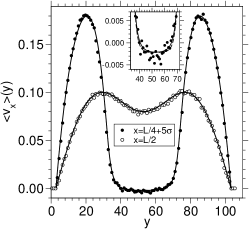
Figure 1: Steady–state streamwise velocity profiles $u(y)=<v_{x}(y)>$ as a function of the crossflow coordinate $y$ at $x=L/4+5\sigma$ (i.e., $5\sigma$ behind the obstacle) and $x=L/2$ as obtained from the MD as indicated. The solid lines are the corresponding results from the LB with resolution $\Delta x=0.25\sigma$. Both the MD and LB curves are averaged along the $x$ direction over a region of $\pm 3\sigma$. The inset shows a magnification of the region around the minimum for the profile at $x=L/4+5\sigma$ (here, the dashed line is the LB result without the averaging along the $x$ direction.

In Fig. 1, we show the steady–state streamwise velocity profile $u(y)\equiv<v_{x}(y)>$ as a function of the crossflow coordinate $y$ at $x=L/4+5\sigma$ and $x=L/2$, for the LB with $\Delta x=0.25\sigma$, as compared to the corresponding profile obtained with the MD simulations. Here, both MD and LB data are averaged along the $x$ direction over a region of $\pm 3\sigma$. This leads to a smoothening of the MD data, but, as the LB results show, has only minor effects on the profiles (this can be infered from the dashed line in the inset of Fig. 1 which shows the LB data without averaging along the $x$ direction). From the data, very good agreement is observed between MD and LB results. Of particular interest is the region around the minimum in the curve for $x=L/4+5\sigma$, where the velocity field $<v_{x}>$ becomes negative. These negative velocities are due to the formation of vortices behind the obstacle. As the inset of Fig. 1 shows, even this region of negative velocities is well reproduced by the LB simulation.

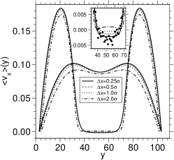
Figure 2: Steady–state streamwise velocity profile $u(y)=<v_{x}(y)>$ as a function of the crossflow coordinate $y$ at $x=L/4+5\sigma$ and $x=L/2$ for the LB simulations with different choices of $\Delta x$ as indicated. As in Fig. 1, the inset shows a magnification of the region around the minimum in the curves for $x=L/4+5\sigma$.

In Fig. 2 the same quantities as in Fig. 1 are shown for the LB runs with different choices of $\Delta x$. From this figure, it is apparent that lack of resolution of the atomic scale $\sigma$ generates significant departures of the LB results from the MD data. This is an informative result, for it implies that microscopic length scales, although absent from the LB description, must nonetheless be resolved if the flow profile away from the walls is to be quantitatively captured by the coarse–grained simulation. This is especially evident in the region where vortices form, i.e. just behind the obstacle. In this region, a quantitative agreement with the MD requires a resolution as high as $\Delta x=0.25\sigma$ (see the inset of Fig. 2).

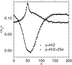
Figure 3: Steady–state streamwise velocity profile $u(y)=<v_{x}(y)>$ as a function of $x$ at $y=H/2$ and $y=H/2\pm 25\sigma$. The symbols show the MD data as indicated. The solid lines are the corresponding LB data with $\Delta x=0.25\sigma$.

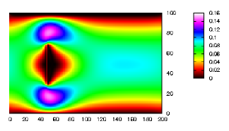
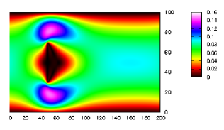
Figure 4: Upper panel: The color map shows the magnitude of the velocity field, $|\vec{u}(x,y)|=\sqrt{<v_{x}>^{2}+<v_{y}>^{2}}$ at steady state as obtained from the MD simulation. Lower panel: The same result as obtained from the LB simulation with $\Delta x=0.25\sigma$ is shown.

In Fig. 3 the streaming velocity $<v_{x}>$ in the direction parallel to the flow is considered for $y=H/2$ and $y=H/2+25\sigma$. In this case LB and MD data were averaged over a region of $\pm 2\sigma$. Note that in the MD case, also the data at $y=H/2-25\sigma$ were used for the average of the profile at $y=H/2+25\sigma$, since the profile is expected to be symmetrical with respect to the central line at $y=H/2$. The comparison between LB and MD shows again a very good agreement. This is not a foregone result, since there are non–trivial features in the vicinity of the obstacle, i.e. around $x=50\sigma$, such as the shoulder at $x=55\sigma$ in the curve for $y=H/2+25\sigma$. Fig. 4 displays the magnitude of the velocity field, $|\vec{u}(x,y)|=\sqrt{<v_{x}>^{2}+<v_{y}>^{2}}$, as obtained from MD (upper plot) and LB (lower plot). Here, it is illustrated that the whole velocity field is quantitatively reproduced.

In conclusion, we have demonstrated an example of a complex nanoscopic fluid flow, in which a spatial handshaking between LB and MD is possible. The mapping of LB onto MD requires a conversion of time and length units from LB to MD and one has to choose an appropriate grid resolution for the LB fluid. For the dense fluid considered in the MD simulation of this work, a grid resolution $\Delta x=0.25\sigma$ is required to reproduce the flow features quantitatively. Remarkably, non–hydrodynamic (finite-Knudsen) effects appear to be silent, at least at steady state. This is likely to be a benefit of the matrix formulation of the collision operator HSB ; MTR , as compared to the more popular single-time relaxation form.

The present results indicate that there appears to be a sound ground for prospective multiscale applications based on the combined use of (multigrid) LB MULBE with MD. For instance, by using multigrid LB with, say, $6$ levels of resolution, one could couple LB with MD at the finest scale $\Delta x_{\rm fine}\sim\sigma$, typically near the boundaries, and then progressively increase the LB mesh–size so as to reach a hundred–fold larger mesh spacing $\Delta x_{\rm bulk}=2^{6}\Delta x_{\rm fine}$ in the bulk flow. On–the–fly time–coupling is obviously more demanding. In fact, our simulations indicate that even with the finest resolution $\Delta x=\sigma/4$, LB is about a factor $2000$ faster than MD (see above). The most direct strategy for ’on–the–fly’ LB–MD coupling is to apply LB everywhere in the fluid domain and leave MD only in small portions, typically in a ratio $1:1000$ to the global domain. Moreover, this factor $1000$ gap could be partially bridged by resorting to very recent time–adaptive LB procedures RASIN . This indicates that, although very demanding, even time–coupling between LB and MD may become soon feasible for the numerical investigation of complex nanoflows.

Of course, several open issues remain. Our comparisons were done at steady state and it is not clear to what extent transient states are correctly described by LB. Moreover, it will be interesting to see whether the LB method still yields a quantitative description in the case of slip–flow and other complex phenomena at the fluid–solid interface. These issues make interesting subjects for forthcoming studies.

- (1) G. Whitesides and A. D. Stroock, Phys. Today 54(6), 42 (2001).
- (2) J. Koplik and J. Banavar, Ann. Rev. Fluid Mech. 27, 257 (1995); J. Koplik, J. Banavar, and I. Willemsen, Phys. Fluids A1, 781 (1989); C. Denniston and M. O. Robbins, Phys. Rev. Lett. 87, 178302 (2001); M. Cieplak, J. Koplik, and J. Banavar, Phys. Rev. Lett. 86, 803 (2001).
- (3) M. Sbragaglia and S. Succi, Phys. Fluids 17, 093602 (2005); S. Ansumali et al., Physica A 359, 289 (2006). S. Ansumali and I. Karlin, Phys. Rev. E, 66, 026311 (2002).
- (4) J. Koplik and J. Banavar, Phys. Fluids 7, 3118 (1995); X. B. Nie et al., J. Fluid Mech. 500, 55 (2004); D. Rapaport and E. Clementi, Phys. Rev. Lett. 57, 695 (1986).
- (5) R. Benzi, S. Succi, and M. Vergassola, Phys. Rep. 222, 145 (1992); S. Chen and G. Doolen, Ann. Rev. Fluid Mech. 130, 329 (1998); S. Succi, The Lattice Boltzmann equation (Oxford Univ. Press, Oxford, 2001).
- (6) F. Higuera, S. Succi, and R. Benzi, Europhys. Lett. 9, 345 (1989).
- (7) D. d’Humiéres, Progress in Aeronautics and Astronautics 159, 450 (1992); P. Lallemand and L.S. Luo, Phys. Rev. E 61, 6546 (2000).
- (8) I. Rasin, S. Succi, and W. Miller, J. Comp. Phys. 206, 453 (2005).
- (9) K. Binder and G. Ciccotti (eds.), Monte Carlo and Molecular Dynamics of Condensed Matter Systems (Italian Physical Society, Bologna, 1996).
- (10) O. Filippova and D. Haenel, J. Comp. Phys. 147, 219 (1998); S. Succi et al., Comp. Sci. Eng., 3(6), 26 (2001).