Spinodal Decomposition in Thin Films: Molecular Dynamics Simulations of a Binary Lennard-Jones Fluid Mixture

Abstract

We use molecular dynamics (MD) to simulate an unstable homogeneous mixture of binary fluids (AB), confined in a slit pore of width $D$. The pore walls are assumed to be flat and structureless, and attract one component of the mixture (A) with the same strength. The pair-wise interactions between the particles is modeled by the Lennard-Jones potential, with symmetric parameters that lead to a miscibility gap in the bulk. In the thin-film geometry, an interesting interplay occurs between surface enrichment and phase separation.

We study the evolution of a mixture with equal amounts of A and B, which is rendered unstable by a temperature quench. We find that A-rich surface enrichment layers form quickly during the early stages of the evolution, causing a depletion of A in the inner regions of the film. These surface-directed concentration profiles propagate from the walls towards the center of the film, resulting in a transient layered structure. This layered state breaks up into a columnar state, which is characterized by the lateral coarsening of cylindrical domains. The qualitative features of this process resemble results from previous studies of diffusive Ginzburg-Landau-type models [S. K. Das, S. Puri, J. Horbach, and K. Binder, Phys. Rev. E 72, 061603 (2005)], but quantitative aspects differ markedly. The relation to spinodal decomposition in a strictly 2-$d$ geometry is also discussed.

I Introduction

Thin fluid films have a broad range of applications in technology as lubricants, protecting layers, for production processes of layered structures in microelectronics, etc. In particular, ultra-thin films have become extremely important in the context of nanotechnology 1 ; 2 ; 3 ; 4 ; 5 ; 6 ; 7 . The interplay of surface effects and finite-size effects with the bulk behavior of these systems poses challenging theoretical problems 8 ; 9 ; 10 ; 11 . A particularly interesting problem in this context is the phase separation of binary (or multi-component) mixtures in thin films, as most materials of practical interest have more than one component, e.g., metallic alloys, ceramics, polymer blends, etc. Phase changes in reduced geometries (e.g., 2-$d$ systems) differ in many aspects from the bulk behavior in three dimensions. The interplay between surface and bulk behavior leads to complex phenomena such as wetting transitions, prewetting and layering transitions, etc. 12 ; 13 ; 14 ; 15 ; 16 ; 17 ; 18 ; 19 ; 20 . These transitions may compete with phase changes that occur in the bulk, such as phase separation in mixtures 21 ; 22 ; 23 ; 24 ; 25 ; 26 . There has been intense study of phenomena such as surface-directed spinodal decomposition (SDSD) or surface-directed phase separation 27 ; 28 ; 29 ; 30 ; 31 ; 32 ; 33 ; 34 ; 35 , but our theoretical understanding of these problems is still incomplete.

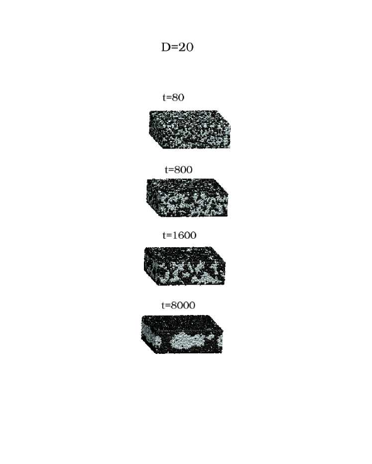
Figure 1: Snapshot pictures of surface-directed spinodal decomposition (SDSD) in a binary (AB) Lennard-Jones (LJ) mixture, which is confined in an $L\times L\times D$ thin-film geometry, with $L=64$, $D=20$. (All lengths are measured in units of the LJ diameter.) Periodic boundary conditions were applied in the lateral directions, while the impenetrable $L\times L$ surfaces (representing the walls of a slit pore) attract the A-particles. The initial condition for this run consisted of a random mixture of equal amounts of A and B, corresponding to a critical quench. Time is also measured in dimensionless LJ units – see Sec. III, where further details of the simulation are specified. The A-particles are marked black, and the B-particles are marked gray. The system quickly develops concentration inhomogeneities ($t=800$), in particular A-rich layers form rapidly at the walls ($t=800$, $t=1600$). The late stages of phase separation are characterized by the lateral coarsening of columnar structures ($t=8000$).

To gain a better understanding of SDSD in thin fluid films, we have undertaken a comprehensive molecular dynamics (MD) simulation of binary mixtures in a slit pore. A preliminary account of our results has been published as a letter dphb . In this paper, we present detailed results from this study. Our MD simulations are based on a symmetric binary (AB) Lennard-Jones (LJ) mixture, for which the bulk phase diagram has been determined to high accuracy 36 . We also have a good understanding of various other properties of this mixture, e.g., static and dynamic response and correlation functions, transport coefficients 36 ; 37 , and the interfacial tension between coexisting A-rich and B-rich phases 38 . Many previous simulation studies of phase-separation kinetics in a thin-film geometry 39 ; 40 have used Ginzburg-Landau (GL) models, and hence lack any direct connection to a microscopic description. Our present modeling bridges the gap between the atomistic description of liquids and the mesoscale domain structures that form as the kinetics of phase separation proceeds (see Fig. 1). This direct approach has the further merit that hydrodynamic interactions are automatically incorporated. It is well-known that these interactions have a pronounced effect on the kinetics of domain growth 21 ; 22 ; 23 ; 24 ; 25 ; 26 ; 41 ; 42 ; 43 ; 44 ; 45 .

In order to account for hydrodynamics in the framework of GL models, rather extensive computations are required 46 ; 47 ; 48 ; 49 ; 50 . The GL approach is appropriate if one is primarily concerned with the scaling behavior of the late-stage domain growth 21 ; 22 ; 23 ; 24 ; 25 ; 26 . But recent work based on lattice Boltzmann simulations questions the quantitative validity of GL models, and reports very slow crossovers extending over many decades in time 53 (however, a “somewhat narrower” crossover region was reported in a subsequent work 53a ). This study also raises questions about some of the previous work on this problem, using the lattice Boltzmann method or related “lattice gas”-approximations to the Navier-Stokes equations of hydrodynamics 54 ; 55 ; 56 ; 57 ; 58 . However, the lattice Boltzmann description is even more remote from an atomistic description of matter than the GL model. Further, it is not clear how one incorporates the proper boundary conditions with respect to complete or partial wetting in such an approach 59 ; 60 . The studies mentioned above are primarily concerned with domain growth in $d=3$. For the $d=2$ case, it is even controversial 61 ; 62 ; 63 to what extent a scaling behavior describes the late stages of coarsening. In view of these problems, it is useful to undertake an MD simulation despite the fact that the accessible scales in length and time are limited. Earlier MD studies of bulk phase separation 64 ; 65 have addressed coarsening in $d=3$ and in $d=2$, but the latter work is somewhat inconclusive 66 . Further, there have only been preliminary MD studies of SDSD in thin films mk93 ; st99 .

The outline of this paper is as follows. In Sec. II, the theoretical background (equilibrium phase behavior of binary mixtures in a thin-film geometry, theory of domain growth, etc.) will be concisely reviewed. In Sec. III, we provide details of our MD methods. In Sec. IV, we present simulation results for SDSD in thin films. Finally, Sec. V concludes this paper with a summary and discussion, including a comparison to the GL approach.

II Theoretical Background

II.1 Equilibrium phase behavior of binary mixtures confined between walls

A homogeneous binary mixture becomes unstable to phase separation when it is quenched into the miscibility gap (see Fig. 2). For a symmetric mixture, the miscibility gap is symmetric with respect to the concentration $x^{\rm crit}_{\rm A}=1/2$.

At the surface of a semi-infinite mixture, one may encounter a wetting transition 12 ; 13 ; 14 ; 15 ; 16 ; 17 ; 18 ; 19 ; 20 . This transition implies a singular behavior of the surface excess free energy $F_{\rm S}$, which is defined as (for a film between two walls at distance $D$) $F_{\rm film}=F_{\rm b}+2F_{\rm S}/D$, $D\rightarrow\infty$, $F_{\rm b}$ being the bulk free energy of the system. Assuming, as done in Fig. 2, that the wetting transition occurs at the surface of B-rich mixtures (caused by the preferential attraction of A-particles to the walls), the transition is characterized by a divergence of the surface excess concentration of A, $x^{\rm surf}_{\rm A}$. This quantity can be obtained from $F_{\rm S}$ via suitable derivatives, or by integrating the concentration profile 12 ; 13 ; 14 ; 15 ; 16 ; 17 ; 18 ; 19 ; 20 ; 70

$$x^{\rm surf}_{\rm A}=\int\limits^{D/2}_{0}\left[x_{\rm A}(z)-x^{(1)}_{\rm A,coex}\right]dz\quad,\quad D\rightarrow\infty\quad,$$ (1)

where $z$ is the distance from the wall, which is located at $z=0$. If the wall is nonwet (or partially wet) 12 ; 13 ; 14 ; 15 ; 16 ; 17 ; 18 ; 19 ; 20 , $x^{\rm surf}_{\rm A}$ tends to a finite value ($x^{\rm surf}_{\rm A,coex}$) when $x_{\rm A}\rightarrow x^{(1)}_{\rm A,coex}$ from the one-phase region. On the other hand, for a wet (or completely wet) wall, $x^{\rm surf}_{\rm A}=\infty$ – corresponding to an infinitely thick A-rich wetting layer coating the wall, separated from the B-rich bulk by a flat interface.

At the coexistence curve $x^{(1)}_{\rm A,coex}$, the surface excess free energy is that of an A-rich phase $F^{\rm B-rich}_{\rm S,coex}$ if the wall is nonwet. For a wet wall, we have $F_{\rm S}=F^{\rm A-rich}_{\rm S,coex}+\gamma_{\rm AB}$, $\gamma_{\rm AB}$ being the interfacial tension between coexisting A-rich and B-rich phases. These quantities also determine the contact angle $\theta$ at which an A-B interface in the nonwet region meets the wall 12 ; 13 ; 14 ; 15 ; 16 ; 17 ; 18 ; 19 ; 20

$$\cos\theta=\frac{\left(F^{\rm B-rich}_{\rm S,coex}-F^{\rm A-rich}_{\rm S,coex}\right)}{\gamma_{\rm AB}}\quad,\quad{\rm if}\quad F^{\rm B-rich}_{\rm S,coex}<F^{\rm A-rich}_{\rm S,coex}+\gamma_{\rm AB}\quad.$$ (2)

If the state of the system is changed such that one increases the temperature but stays always at the coexistence curve $x^{(1)}_{\rm A,coex}$, one encounters a wetting transition at temperature $T_{\rm w}$ (Fig. 2), where the state of the wall changes from nonwet $(T<T_{\rm w})$ to wet $(T>T_{\rm w})$. This transition may be of second order (Fig. 2a) or first order (Fig. 2b). In the second-order case, $x^{\rm surf}_{\rm A}$ diverges continuously when $T\rightarrow T_{w}^{-}$, while otherwise there is a discontinuous jump in $x^{\rm surf}_{\rm A}$ from a finite value at $T_{w}^{-}$ to $\infty$ at $T_{w}^{+}$. In the first-order case, there is also a prewetting transition in the one-phase region (Fig. 2b), where the thickness of the A-rich surface layer jumps from a smaller value to a larger (but finite) value. This line of prewetting transitions ends in a prewetting critical point.

This brief review of wetting phenomena provides the basis to understand the equilibrium behavior of binary mixtures in thin films 71 ; 72 ; 73 ; 74 ; 75 ; 76 ; 77 ; 78 ; 79 ; 80 . If the walls are neutral (i.e., it has the same attractive interactions with both A-particles and B-particles), the critical concentration remains $x^{\rm crit}_{\rm A}=1/2$. However, the critical temperature $T_{\rm c}(D)$ is lowered 71 ; 76 ; 77 relative to the bulk:

$$T_{\rm c}-T_{\rm c}(D)\propto D^{-1/\nu},$$ (3)

where $\nu\simeq 0.629$ 68 ; 69 is the critical exponent of the correlation length $\xi$ of concentration fluctuations (in the universality class of the $d=3$ Ising model). Note, however, that critical correlations at fixed finite $D$ can become arbitrarily long-range only in the lateral direction parallel to the film. Thus, the transition at $T_{\rm c}(D)$ belongs to the class of the $d=2$ Ising model. The states below the coexistence curve of the thin film correspond to two-phase equilibria characterized by lateral phase separation.

When there is a preferential attraction of A-particles to the walls, the phase diagram of the thin film is no longer symmetric with respect to $x_{\rm A}=1/2$, although we did assume such a symmetry in the bulk. The shift of $x_{\rm A}^{\rm crit}$ and the resulting change of the coexistence curve, is the analog of capillary condensation of gases 74 ; 81 for binary mixtures.

The coexisting phases in the region below the coexistence curve of the thin film are inhomogeneous in the direction perpendicular to the walls (see Fig. 2c). In the A-rich phase, we expect only a slight enhancement of the order parameter $\psi(z)$, which is defined in terms of the densities $n_{\rm A}(z)$, $n_{\rm B}(z)$ of A and B particles as

$$\psi(z)=\frac{n_{\rm A}(z)-n_{\rm B}(z)}{n_{\rm A}(z)+n_{\rm B}(z)}\quad.$$ (4)

In the B-rich phase, however, we expect pronounced enrichment layers. As $D\rightarrow\infty$, the thickness of these layers diverges for $T>T_{\rm w}$ but stays finite for $T<T_{\rm w}$. In a film of finite thickness, the width of A-rich surface layers also stays finite, e.g., for $T>T_{\rm w},~{}x_{\rm A}^{\rm surf}\propto\ln D$ for short-range surface forces, while $x^{\rm surf}_{\rm A}\propto D^{1/3}$ for non-retarded van der Waals’ forces 76 ; 82 . Thus, the wetting transition is always rounded off in a thin film. The prewetting line (Fig. 2b) does have an analog in films of finite thickness $D$, for sufficiently large $D$. This transition splits into a two-phase region at small $x_{\rm A}$ between the thin-film triple point and the thin-film critical point on the B-rich side. This two-phase region corresponds to a coexistence between B-rich phases with A-rich surface layers, both of which have finite (but different) thickness. As $D\rightarrow\infty$, the thin-film critical point on the B-rich side moves into the prewetting critical point, while the thin-film triple point merges with the first-order wetting transition. On the other hand, when $D$ becomes small, the thin-film critical point and the thin-film triple point may merge and annihilate each other. For still smaller $D$, the thin-film phase diagram then has the shape shown in Fig. 2a, although one has first-order wetting in the semi-infinite bulk (Fig. 2b).

Finally, we comment on the state encountered below the bulk coexistence curve, but above the coexistence curve of the thin film. When one crosses the bulk coexistence curve, there is a rounded transition towards a layered (stratified) structure with two A-rich layers at the walls and a B-rich layer in the middle. The temperature range over which this rounded transition is smeared is also of order $\Delta T\propto D^{-1/\nu}$ around $T_{\rm c}$. Hence, for large $D$, this segregation in the direction normal to the walls may easily be mistaken (in experiments or simulations) as a true (sharp) phase transition. We stress that this is not a true transition – one is still in the one-phase region of the thin film, although the structure is strongly inhomogeneous! The situation qualitatively looks like the concentration profile shown in the upper part of Fig. 2c. The difference is that, for $D\rightarrow\infty$, the thickness of true wetting layers scales sub-linearly with $D$, as noted above. However, for phase separation in the normal direction which gradually sets in when one crosses the bulk coexistence curve, one simply has A-rich domains of macroscopic dimensions (proportional to $D$) adjacent to both walls. Unfortunately, the layers resulting in this stratified structure are often referred to as “wetting layers” in the literature, although this is completely misleading. We reiterate that A-rich wetting layers only form when a B-rich domain extends to the surface, which is not the case here.

We also caution the reader that a picture in terms of A-rich layers at the walls and a B-rich domain in the inside of the film is an over-simplification because the thickness of the domain walls cannot really be neglected in the region $T_{\rm c}(D)<T<T_{\rm c}$, where a stratified structure occurs in equilibrium. This is seen from the relation $\xi\propto(1-T/T_{\rm c})^{-\nu}$, in conjunction with Eq. (3), which shows that $\xi\sim O(D)$ at $T_{\rm c}(D)$. Thus, domains and domain walls are not well-distinguished in the region under consideration, since the interfacial width is $O(\xi)$ 20 ; 70 .

When the interface between A-rich and B-rich domains is treated as a sharp kink (this approximation is popular in theoretical treatments of wetting 12 ; 13 ; 14 ; 15 ; 16 ; 17 ; 18 ; 19 ; 20 ), one might think that a sharp wetting transition could still be described in terms of the vanishing of the contact angle $\theta$ as $T\rightarrow T_{\rm w}^{-}$ (Fig. 2c). However, it is clear that for a correct treatment the finite width of the interface needs to be taken into account. Thus, for finite $D$, the contact angle in Fig. 2c is ill-defined, and the transition between the two states depicted in Fig. 2c is smooth, because a B-rich nonwet domain may also have a thin A-rich layer at its surface ($x^{\rm surf}_{\rm A}$, in general, is nonzero). One should also note that the contact “line” is distorted by line tension effects when it hits the wall, and the line tension of the interface at the wall would also modify Eq. (2) 83 ; 84 ; 85 . The difficulty of estimating the contact angle in finite geometries is well-known from studies of nanoscopic droplets 86 ; 87 .

The central conclusion in this subsection is that in the final equilibrium to which, for times $t\to\infty$ and for small $D$, the thin film evolves, there is no fundamental difference whether or not we are above or below the wetting transition temperature, but it matters whether $T<T_{\rm c}(D)$ or $T>T_{\rm c}(D)$.

II.2 Bulk phase separation of binary fluid mixtures

Next, we review our understanding of the kinetics of phase separation in bulk fluid mixtures which are rendered thermodynamically unstable by a rapid quench (at $t=0$) into the miscibility gap (see Fig. 2). The initial state ($t\leq 0)$ is spatially homogeneous, apart from small-scale concentration inhomogeneities. The final equilibrium state consists of macroscopic domains of the two coexisting phases, with relative amounts determined by the lever rule. We are interested in the evolution from the initial homogeneous state to the final segregated state. For quenches below the spinodal curve, the homogeneous system is unstable and decomposes via the spontaneous growth of long-wavelength concentration fluctuations 21 ; 22 ; 23 ; 24 ; 25 ; 26 (spinodal decomposition). Understanding the full time evolution from the initial stages to the late stages of coarsening is a formidable problem, and is typically accessed by large-scale simulations of coarse-grained models.

Nevertheless, there exist some cases in which simple domain growth laws can be obtained from analytical considerations 42 ; 43 ; 44 ; 45 ; 93 ; 94 . The evaporation-condensation mechanism of Lifshitz and Slyozov (LS) 93 corresponds to a situation where a population of droplets of the minority phase (say, A) is in local equilibrium with the surrounding supersaturated majority phase. The LS mechanism leads to a growth law (valid for dimensionality $d>1$) $\ell(t)\propto t^{1/3}$, $t\rightarrow\infty$, where $\ell(t)$ is the linear dimension of the droplets.

The droplet diffusion-coagulation mechanism 94 is specific to fluid mixtures, and is based on Stokes law for the diffusion of droplets, yielding 94 $\ell(t)\propto(t/\eta)^{1/d}$.

A faster mechanism of domain growth in fluids was proposed by Siggia 42 , who studied the coarsening of interconnected domain structures via the deformation and break-up of tube-like regions, considering a balance between the surface energy density $\sim\gamma_{\rm AB}/\ell$ and the viscous stress $\sim 6\pi\eta v_{\ell}/\ell$ 25 . Thus, $v_{\ell}\propto\gamma_{\rm AB}/\eta$ and $\frac{d\ell}{dt}\propto v_{\ell}$, or $\ell(t)\propto\frac{\gamma_{\rm AB}}{\eta}t$ in $d=3$. In $d=2$, the analog of this hydrodynamic mechanism is controversial. San Miguel et al. 43 argue that strips ($d=2$ analogs of tubes) are stable under small perturbations, in contrast to the $d=3$ case. For critical volume fractions, an interface diffusion mechanism is proposed which yields $\ell(t)\propto t^{1/2}$, i.e., the same growth law as the Brownian coalescence mechanism of droplets in $d=2$ (see above). On the other hand, Furukawa 44 ; 62 argues for a linear relation $\ell(t)\propto t$ in $d=2$ as well. However, recently there is growing evidence 61 ; 62 ; 63 that different characteristic length scales in $d=2$ may exhibit different growth exponents, suggesting that there is no simple dynamical scaling of domain growth in $d=2$!

Finally, we remark that the above growth laws do not constitute the true asymptotic behavior, either in $d=2$ or $d=3$. Rather, these results only hold for low enough Reynolds numbers 25 . For $\ell\gg\ell_{\rm in}=\eta^{2}/(n\gamma_{\rm AB})$, the so-called inertial length 25 , one enters a regime where the surface energy density $\gamma_{\rm AB}/\ell$ is balanced by the kinetic energy density $nv^{2}_{\ell}$. This yields the following growth law for the inertial regime 25 ; 44 :

$$\ell(t)\propto\left(\frac{\gamma_{\rm AB}}{n}\right)^{1/3}t^{2/3}\quad,$$ (5)

which is valid for both $d=2$ and $d=3$. In $d=2$, evidence for both $\ell(t)\propto t^{1/2}$ and $\ell(t)\propto t^{2/3}$ has been reported, but the conditions under which such power laws hold in $d=2$ are still not clear 50 ; 61 ; 62 ; 63 ; 64 ; 65 ; 66 .

II.3 Ginzburg-Landau model of surface-directed spinodal decomposition

In this subsection, we briefly discuss a coarse-grained description of binary mixtures in a thin-film geometry, which can reproduce the phase diagrams shown in Fig. 2. This description can also be used to obtain a model for the kinetics of phase separation in a confined geometry. Our starting point is a mean-field description of a binary mixture near its critical point, where one introduces a local order parameter $\psi(\vec{\rho},z)$. (Here, $\vec{\rho}$ represents the coordinates parallel to the walls, and $z$ is the coordinate in the perpendicular direction, as before.) The surfaces of the thin film $S_{1}$ and $S_{2}$ are located at $z=0$ and $z=D$, respectively.

We denote the order parameter describing the bulk coexistence curve as $\psi_{\rm b}$, and define $\psi^{\prime}(\vec{\rho},z)=\psi(\vec{\rho},z)/\psi_{\rm b}$. Further, we measure distances $\vec{\rho},z,D$ in units of $\xi$. Then, the dimensionless free-energy functional of a binary mixture in a thin-film geometry can be written as a sum of a bulk term $F_{\rm b}$ and two surface terms 40 , $F[\psi]=F_{\rm b}[\psi]+F_{S_{1}}[\psi]+F_{S_{2}}[\psi]$, where we have dropped the prime on $\psi^{\prime}$. Here, we have

$$F_{\rm b}[\psi]=\int d\vec{\rho}\int\limits^{D}_{0}dz\left[-\frac{\psi^{2}}{2}+\frac{\psi^{4}}{4}+\frac{1}{4}(\vec{\nabla}\psi)^{2}+V(z)\psi\right]\quad.$$ (6)

The terms $F_{S_{1}}$ and $F_{S_{2}}$ are obtained as integrals over the surfaces $S_{1}$ and $S_{2}$:

$$F_{S_{1}}=\int\limits_{S_{1}}d\vec{\rho}\left\{-\frac{g}{2}[\psi(\vec{\rho},0)]^{2}-h_{1}\psi(\vec{\rho},0)-\gamma\psi(\vec{\rho},0)\frac{\partial\psi}{\partial z}\bigg{|}_{z=0}\right\}\quad,$$ (7)

and analogously for $F_{S_{2}}$.

In Eq. (6), we have included a $z$-dependent surface potential which arises due to the surfaces. In our subsequent discussion, we will consider symmetric power-law potentials:

$$V(z)=-V_{0}\left[(z+1)^{-p}+(D+1-z)^{-p}\right]\quad,$$ (8)

which satisfy $V(z)=V(D-z)$. The potentials are taken to originate behind the surfaces so as to avoid singularities at $z=0,D$.

The terms $F_{S_{1}}$, $F_{S_{2}}$ represent the surface excess free-energy contributions due to local effects at the walls, with $g$ and $\gamma$ phenomenological parameters 31 ; 35 ; 70 ; 95 . The dimensionless surface fields in $F_{S_{1}}$ and $F_{S_{2}}$ are $h_{1}=-V(0)$ and $h_{2}=-V(D)$, respectively. The one-sided derivatives appear in $F_{S_{1}}$ and $F_{S_{2}}$ due to the absence of neighboring atoms for $z<0$ and $z>D$.

Let us first consider the limit $D\rightarrow\infty$. For the long-range surface potential Eq. (8), only first-order wetting transitions are possible 14 . For power-law potentials as in Eq. (8), an approximate theory 35 predicts that the wetting transition occurs when $2V_{0}/(p-1)=\gamma_{\rm AB}$.

For finite values of $D$, one can obtain phase diagrams of thin films (as shown schematically in Fig. 2) by minimizing the free-energy functional in Eqs. (6)-(8). However, this requires numerical work 71 ; 78 . We also note that the $\psi^{4}$-model cannot describe either the low-temperature region (where complete separation between A and B occurs), or the non-mean-field critical behavior.

We next discuss the dynamics of phase separation in thin films. First, let us establish the dynamical equations which govern phase separation in the bulk for the diffusion-driven case. The local order parameter $\psi(\vec{r},t)$ is conserved, and obeys the continuity equation 21 ; 22 ; 23 ; 24 ; 25 ; 26 :

$$\frac{\partial}{\partial t}\psi(\vec{r},t)=-\vec{\nabla}\cdot\vec{J}(\vec{r},t)\quad,$$ (9)

The current $\vec{J}(\vec{r},t)$ contains contributions from the local chemical potential difference $\mu(\vec{r},t)$, and from statistical fluctuations, $\vec{\theta}(\vec{r},t)$:

$$\vec{J}(\vec{r},t) = -\vec{\nabla}\mu(\vec{r},t)+\vec{\theta}(\vec{r},t)\quad,$$

$$\mu(\vec{r},t) = \frac{\delta F}{\delta\psi(\vec{r},t)}\quad.$$ (10)

Using the $\psi^{4}$-free-energy functional in Eq. (6), we obtain the dynamical model:

$$\frac{\partial}{\partial t}\psi(\vec{r},t)=\vec{\nabla}\cdot\left\{\vec{\nabla}\left[-\psi+\psi^{3}-\frac{1}{2}\nabla^{2}\psi+V(z)\right]+\vec{\theta}(\vec{r},t)\right\},\quad 0<z<D.$$ (11)

We assume that the noise $\vec{\theta}$ is a Gaussian white noise, obeying the relations $\langle\vec{\theta}(\vec{r},t)\rangle=0$ and $\langle\theta_{i}(\vec{r}\;^{\prime},t^{\prime})\theta_{j}(\vec{r}\;^{\prime\prime},t^{\prime\prime})\rangle=2\epsilon\delta_{ij}\delta(\vec{r}\;^{\prime}-\vec{r}\;^{\prime\prime})\delta(t^{\prime}-t^{\prime\prime})$, where the indices $i,j$ denote the Cartesian components of vector $\vec{\theta}$. Note that the time units have been chosen such that the diffusion constant in Eq. (II.3) is unity. With respect to the dynamical behavior in the critical region, Eq. (11) corresponds to model B in the Hohenberg-Halperin classification 99 . However, statistical fluctuations are irrelevant for the late stages of spinodal decomposition po88 : The deterministic model obtained by setting $\epsilon=0$ in Eqs. (9)-(II.3) also yields the LS growth law (see Sec. IIB) in the late stages of domain growth.

One can incorporate hydrodynamic effects, as is appropriate for fluid mixtures, by including a velocity field $\vec{v}(\vec{r},t)$ 99 , but this will not be further considered here.

The above models describe coarsening kinetics in the bulk. When one deals with SDSD in thin films, the model needs to be supplemented by boundary conditions at the surfaces 28 ; 100 . The first boundary condition expresses the physical requirement that the $z$-component of the flux at the surfaces must vanish:

$$J_{z}(\vec{\rho},0,t)=\left\{-\frac{\partial}{\partial z}\left[-\psi+\psi^{3}-\frac{1}{2}\nabla^{2}\psi+V(z)\right]+\theta_{z}\right\}_{z=0}=0\quad,$$ (12)

and similarly for $z=D$. The second boundary condition describes the evolution of the surface order parameter. Since this quantity is not conserved, it is described by a relaxational kinetics of model A type 99 :

$$\tau_{0}\frac{\partial}{\partial t}\psi(\vec{\rho},0,t) = -\frac{\delta F}{\delta\psi(\vec{\rho},0,t)}$$ (13)

$$= h_{1}+g\psi(\vec{\rho},0,t)+\gamma\frac{\partial\psi}{\partial z}\bigg{|}_{z=0}\quad.$$

An analogous equation can be written down for the relaxation of $\psi(\vec{\rho},D,t)$. Here, $\tau_{0}$ sets the time-scale of this nonconserved kinetics. Since $\psi(\vec{\rho},0,t)$ relaxes much faster than the order parameter in the bulk, it is reasonable to set $\tau_{0}=0$ 35 . Then, the dynamics as well as the statics is controlled by two surface parameters, $h_{1}/\gamma$ and $g/\gamma$. During the early stages of SDSD, the fast relaxation of the order parameter at the surfaces provides a boundary condition for the phase of concentration waves that grow in the thin film. In the bulk, the random orientations and phases of these growing waves do not yield a systematic evolution of the average order parameter. However, the surface-directed concentration waves add up to give an average oscillatory concentration profile near the surfaces of a thin film 27 ; 28 ; 29 ; 30 ; 31 ; 32 ; 33 ; 34 ; 35 ; 39 ; 40 .

Our early work on SDSD in thin films 39 omitted both hydrodynamic interactions and the noise in Eq. (II.3), and focused on the $d=2$ case. In recent work 40 , we have studied the $d=3$ case using the GL model in Eq. (11) with the noise term, in conjunction with the boundary conditions in Eqs. (12)-(13). In Sec. IV, we will compare our MD results with results from this study. The details of the GL simulation are as follows. We implemented an Euler-discretized version of Eqs. (11), (12)-(13) on an $L\times L\times D$ lattice. The discretization mesh sizes were $\Delta x=1$ and $\Delta t=0.02$. The surface potential was of the form in Eq. (8) with $p=3$, which corresponds to a non-retarded van der Waals’ interaction between the surfaces and a particle in $d=3$. The parameter values were $g=-0.4,\gamma=0.4$, and $V_{0}=0.325$ for $D=5$ and $V_{0}=0.11$ for $D=10$, corresponding to a partially wet surface in equilibrium. We stress that, for a fluid mixture, the above diffusive model is relevant during the early stages of phase separation 21 ; 22 ; 23 ; 24 ; 25 ; 26 , but is not expected to yield useful results for the intermediate and late stages of domain growth.

III Model and Molecular Dynamics Methods

For our MD study, we consider a fluid of point particles located in continuous space in a box of volume $L\times L\times D$. We apply periodic boundary conditions in the $x$ and $y$ directions, while impenetrable walls are present at $z=0$ and $z=D$. These walls give rise to an integrated LJ potential ($\alpha$ = A,B):

$$u_{\rm w}(z)=\frac{2\pi n\sigma^{3}}{3}\epsilon_{\rm w}\left[\frac{2}{15}\left(\frac{\sigma}{z^{\prime}}\right)^{9}-\delta_{\alpha}\left(\frac{\sigma}{z^{\prime}}\right)^{3}\right]\quad,$$ (14)

where $n$ is the reference density of the corresponding bulk fluid 36 ; 37 ; 38 , $\sigma$ is the LJ diameter of the particles, and $\epsilon_{\rm w}$ is an energy scale for the strength of the wall potentials. Further, $\delta_{\rm A}=1$ and $\delta_{\rm B}=0$, so A-particles are attracted by the walls while B-particles are not. The coordinate $z^{\prime}=z+\sigma/2$ for the wall at $z=0$, and $z^{\prime}=D+\sigma/2-z$ for the wall at $z=D$. Therefore, the singularities of $u_{\rm w}(z)$ do not occur within the range $0\leq z\leq D$ but rather at $z=-\sigma/2$ and $z=D+\sigma/2$, respectively.

The particles in the system interact with LJ potentials:

$$u(r_{ij})=4\epsilon_{\alpha\beta}\left[\left(\frac{\sigma_{\alpha\beta}}{r_{ij}}\right)^{12}-\left(\frac{\sigma_{\alpha\beta}}{r_{ij}}\right)^{6}\right],\quad\quad r_{ij}=|\vec{r}_{i}-\vec{r}_{j}|,$$ (15)

where $\alpha,\beta={\rm A},{\rm B}$. The LJ-parameters $(\epsilon_{\alpha\beta},\sigma_{\alpha\beta})$ are chosen as follows:

$$\sigma_{\rm AA}=\sigma_{\rm AB}=\sigma_{\rm BB}=\sigma,$$

$$\epsilon_{\rm AA}=\epsilon_{\rm BB}=\epsilon,\quad\epsilon_{\rm AB}=\frac{\epsilon}{2}\quad.$$ (16)

The units of length, temperature, and energy are chosen such that $\sigma=1$, $\epsilon=1$, $k_{B}=1$. The masses of the particles are chosen to be equal, $m_{\rm A}=m_{\rm B}=m=1$. Thus, the MD time unit 101 ; 102 ; 103 :

$$t_{0}=\left(\frac{m\sigma^{2}}{48\epsilon}\right)^{1/2}=\frac{1}{\sqrt{48}},$$ (17)

becomes a dimensionless number. To speed up the calculations, the LJ potential is truncated at $r_{ij}=2.5\,\sigma$ and shifted to zero there, as usual 101 . To ensure that our study of fluid-fluid phase separation is not affected by other phase transitions (e.g., liquid-gas or liquid-solid transitions), we work with bulk density $n=1.0$ and focus on temperatures $T>1.0$. In principle, in thin films one could have a wall-induced crystallization at temperatures above the bulk melting temperature: however, we have not seen any evidence for such an effect in our model. In our previous work on the bulk behavior of the same model 36 ; 37 ; 38 , we found that the critical temperature for bulk phase separation is $T_{\rm c}\simeq 1.638$. Here, we present results from simulations of quenching experiments to $T=1.1$. At this temperature, the bulk phase separation is essentially complete. In addition, the bulk correlation length $\xi\simeq 1$ (i.e., one LJ diameter) within the relative accuracy of about 5% to which it can be determined 36 . Further, material parameters which enter the theories reviewed in Sec. II (e.g., the interfacial tension $\gamma_{\rm AB}$, the shear viscosity $\eta$) are explicitly known as well. The appropriate values are $\gamma_{AB}\simeq 0.9$ (see Ref. 38 ) and $\eta\simeq 7$ (see Ref. 36 ). (Recall that these quantities are measured in LJ units and hence are dimensionless.) The availability of most material parameters for our system is a distinct advantage of our atomistic model in comparison to coarse-grained models, where it is often unclear what ranges of effective parameters correspond to physically reasonable choices.

The strength of the wall-particle interaction is taken as $\epsilon_{\rm w}=0.005$, which corresponds to partially wet walls at $T=1.1$. To find the precise location of the wetting transition for our model would require a major computational effort, and this has not been attempted. Recall that one expects $T_{\rm w}\rightarrow T_{\rm c}$ when $\epsilon_{\rm w}\rightarrow 0$ – this was the motivation for choosing a rather small value of $\epsilon_{\rm w}$ in our study. However, due to the special choices made [such as Eq. (III)], for the sake of simplicity, it would be premature to try to explicitly relate our model to a specific real system.

The lateral size $L$ of the simulated systems must be large enough that the laterally inhomogeneous structures that form during segregation are not affected by finite-size effects. Therefore, we chose $L=128$ for the thinnest film in our study ($D=5$) and $L=64$ for the thicker ones ($D=10,20$). As the confining potentials diverge at $z=-\sigma/2$ and $z=D+\sigma/2$ ($\sigma=1$), the volume in which particles can be is $V=L^{2}(D+1)$. We will report results from three sets of simulations, with $D=5,L=128$ ($N=98304$ particles); $D=10,L=64$ ($N=45056$); and $D=20,L=64$ ($N=86016$). Thus, the particle density is $n=1$ in all these cases. For the range of times studied here ($t\leq 8000$), test runs with other linear dimensions showed that our choices of $L$ are large enough to eliminate finite size effects, within the limits of our statistical accuracy. Of course, for a study on larger time scales also larger system sizes would be required!

The initial states of the simulations need to be carefully prepared. We equilibrated a fluid of $N$ particles (with $N_{\rm A}=N_{\rm B}=N/2$) in the specified volume at a very high temperature ($T=5$), with periodic boundary conditions in all directions. The equilibration time was $10^{5}$ MD time steps. At this high temperature, only very weak chemical correlations develop among the particles. We use the standard velocity Verlet algorithm 101 ; 102 ; 103 with a time step of 0.02, and apply the Nosé-Hoover algorithm 101 ; 102 ; 103 for thermalization.

At time $t=0$, the wall potentials are introduced, and the temperature is quenched to $T=1.1$. This is done by rescaling the velocities, and by setting the temperature of the Nosé-Hoover thermostat to the new temperature. Of course, in a real experiment, the temperature of a fluid confined in a small slit pore would be controlled via the thermal energy of the solid walls forming the pore. Therefore, no instantaneous quench (on picosecond or nanosecond time-scales) is possible. However, the structure formation occurring in a binary fluid with a finite quench rate is a complication that we disregard here.

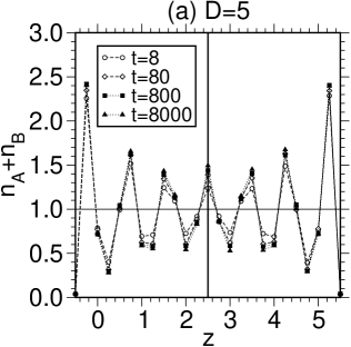
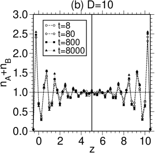
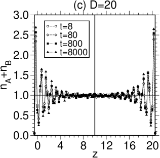
Figure 3: Profiles of the total density $n(z)=n_{\rm A}(z)+n_{\rm B}(z)$ vs. $z$ for (a) $D=5$, (b) $D=10$, and (c) $D=20$. We show data for four different times $t$ (in units of $t_{0}$), as indicated. The vertical line in each frame indicates the mid-plane of the film at $z=D/2$. The wall potentials diverge at $z=-1/2$ and $z=D+1/2$ [see Eq. (14)], so the particles can range over a distance $(D+1)$ in the $z$-direction. All lengths are measured in units of $\sigma$, and hence are dimensionless.

It is also relevant to discuss our procedure of introducing the walls together with the quench at time $t=0$. In this case, the fluid is translationally invariant for $t<0$, but loses this invariance in the $z$-direction for $t>0$. However, we have found that the typical oscillatory density profiles near the walls (“layering”) already develop during the first few MD time steps after the quench – see Fig. 3. For $D=5$, we recognize 7 well-developed layers and there is no region of constant density in such an ultra-thin film. However, for $D=10$, the region from $z\simeq 4$ to $z\simeq 6$ has an almost constant density $n(z)=n_{\rm A}(z)+n_{\rm B}(z)\simeq n=1$. For the $D=20$ case, this constant density region covers about half of the film thickness, extending from $z\simeq 5$ to $z\simeq 15$. Note that the layer distance in Fig. 3 is slightly less than $\sigma$, although $\sigma$ coincides with the position of the first peak of the radial distribution functions in the bulk 36 . We introduce the walls together with the quench at time $t=0$ to make the initial state of the quench (random distribution of $A$ and $B$ particles everywhere in the system, also close to the wall) comparable to that of the Ginzburg-Landau model (where we quench from a state at “infinite temperature”).

It has been emphasized 102 that MD simulations constitute a method to explore hydrodynamic phenomena, and are competitive with coarse-grained methods. In principle, this is only true for a microcanonical MD in the NVE ensemble where the energy $E$ is strictly conserved. However, here we use the Nosé-Hoover thermostat 101 ; 102 ; 103 , i.e., we integrate the following equations of motion for the coordinates of the particles $\vec{r}_{i}(t)$ (with ${\dot{\vec{r}}}_{i}=d\vec{r}_{i}/dt=\vec{v}_{i}$):

$${\ddot{\vec{r}}}_{i}(t)=\frac{\vec{f}_{i}}{m_{i}}-\zeta(t)\vec{r}_{i},$$ (18)

$$\dot{\zeta}(t)=\frac{1}{Q}\left(\sum\limits_{i=1}^{N}m_{i}{\vec{v}_{i}}^{~{}2}-3Nk_{B}T\right)\quad.$$ (19)

Here, $Q$ is the fictitious mass of the thermostat, which was set to $Q=100$. In the limit $Q=\infty$, we have $\zeta(t)=0$ and then we recover the strict conservation of energy and momentum, on which the equations of hydrodynamics are based. For finite $Q$, we have $\langle\zeta(t)\rangle=0$. However, the fluctuating damping term disturbs hydrodynamics slightly. For this reason, in our earlier study of isothermal transport coefficients in the bulk 36 ; 37 , we have used strictly microcanonical runs. However, the ensemble of initial states was generated by Monte Carlo simulations in the semi-grand-canonical ensemble, ensuring thus a strict validity of all conservation laws in conjunction with averaging in the NVT ensemble. In the context of a thin fluid film confined in a slit between solid walls formed from vibrating atoms, neither momentum nor energy (of the fluid film) are conserved, and the walls do act as a thermostat. Of course, in a more realistic model, this thermostatting action of the walls applies only to those fluid particles which are close to one of the walls, and not on particles near the center of the film (which are only thermostatted indirectly via heat conduction). In situations far from local equilibrium (such as strongly sheared fluids 103 ; 104 ), there is indeed a noticeable difference between the effects of wall thermostats and the Nosé-Hoover thermostat. However, we do not expect any such problem here, since the time-scales for domain coarsening are much larger than the time-scales associated with heat conduction.

In simulations of domain growth, one encounters the problem of large statistical fluctuations, and quantities such as the equal-time correlation function $C(\vec{r},t)$ exhibit lack of self-averaging 105 . [Unlike the equilibrium case, $C(\vec{r},t)$ explicitly depends on the time $t$ after the quench.] Such quantities can only be sampled if a number of independent runs are performed and averaged over. All statistical quantities presented here are obtained as averages over three independent runs.

IV Numerical Results

Let us begin with a discussion of the laterally averaged order parameter profiles, $\psi_{\rm av}(z,t)$ vs. $z$ (see Fig. 4). These are obtained from our MD simulations by averaging individual profiles for $\psi(x,y,z,t)$ vs. $z$ along the $x$ and $y$ directions, and further averaging over independent runs. The morphology of these SDSD profiles consists of an A-rich wetting layer at the surface, followed by a depletion layer in A, etc. One can see that the order parameter at the surface has already increased to a rather large value at early times, due to the preferential attraction of the A-particles to the walls. These A-particles are removed from the adjacent regions in the interior of the film, resulting in local minima in $\psi_{\rm av}(z,t)$ (A-depletion layers). As time proceeds, these minima move towards the center, and also become more pronounced. In the $D=5$ case, the SDSD waves coalesce rapidly and only a single minimum in the center is left by $t=640$. In the $D=10$ case, distinct SDSD waves are visible till $t\simeq 1000$. At $t=2000$ (see Fig. 4d), the waves have merged to give a layered structure with a single minimum. In both cases, the layered structure is transient and breaks up into a columnar structure which coarsens laterally (see Fig. 1). Of course, even in this asymptotic state, the walls remain A-rich and the film center is B-rich. This behavior is reminiscent of the SDSD profiles seen in GL studies of this problem 28 ; 31 ; 39 ; 40 , and corresponding experiments 30 . In the present MD simulations, only a single depletion minimum is observed near each wall – statistical fluctuations of the local position of the boundaries between the depletion layers and adjacent enrichment layers wipe out any further systematic variation of the concentration profiles.

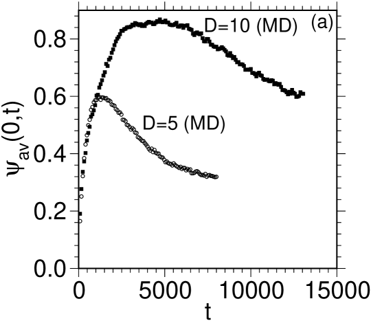
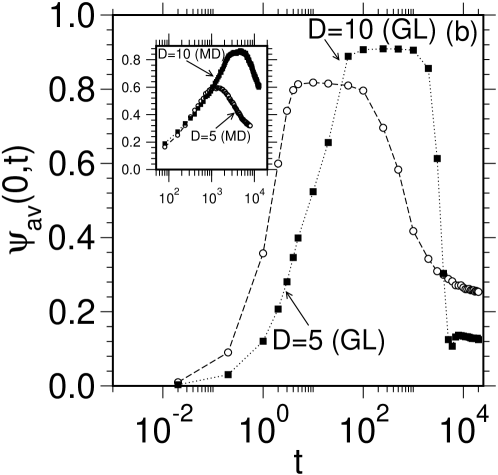
Figure 5: (a) Time-dependence of the local order parameter $\psi_{\rm av}(0,t)$ at the surface $z=0$. We show data for $D=5$ and $D=10$. Note that we have averaged the MD data over a layer of thickness $\Delta z=1$ to estimate $\psi_{\rm av}(0,t)$. (b) Time-dependence of $\psi_{\rm av}(0,t)$, obtained from the Ginzburg-Landau (GL) simulations described in Sec. II.C 40 . The GL data was obtained as an average over 5 independent runs with $L=256$. We plot the data on a log-linear scale. The inset shows the MD data from (a), also on a log-linear scale.

It is also interesting to examine the evolution of the local order parameter $\psi_{\rm av}(0,t)$ at the surface $z=0$ (see Fig. 5a) or $z=D$ (which is analogous to Fig. 5a). Note that we have averaged the MD data over a layer of thickness $\Delta z=1$ to estimate $\psi_{\rm av}(0,t)$ (whereas for the calculation of $\psi_{\rm av}(z,t)$ in Fig. 4 $\Delta z=0.25$ was used). The quantity $\psi_{\rm av}(0,t)$ rises rapidly, and reaches a maximum at about two decades, before it starts decreasing. The rapid rise is expected from the phenomenological theory (see Sec. II C). Of course, due to the lack of conservation of the local order parameter adjacent to the walls, there is an immediate response to the surface potential at the wall. For both $D=5$ and $D=10$, even runs up to $t=2\cdot 10^{4}$ do not suffice to estimate the final values of $\psi_{\rm av}(0,t)$ clearly. This non-monotonic relaxation is a consequence of the structural rearrangement of the concentration inhomogeneities in the films. Figure 5b shows corresponding data for $\psi_{\rm av}(0,t)$ vs. $t$ from our recent simulations, using the GL model described in Sec. II.C 40 . (Note that a logarithmic time-axis is chosen in Fig. 5b.) The behavior of the GL data is qualitatively similar to that of the MD results. However, a pronounced intermediate plateau is formed in the GL case, whereas the MD data only show a maximum – see the inset of Fig. 5b, which plots the data from Fig. 5a on a logarithmic time-scale. The reason for this difference lies in the formation of a long-lived metastable layered state with pronounced A-rich layers in the GL case, which is not observed in the MD simulations.

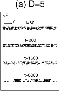
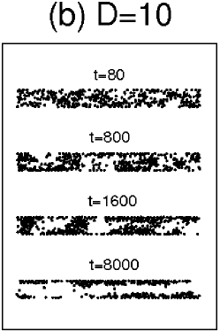
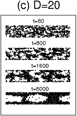
Figure 6: Snapshots of the concentration distribution in cross-section slices (of linear dimensions $\sigma\times L\times D$) through the films, for (a) $D=5$, (b) $D=10$, and (c) $D=20$. The cross-section was centered at $x=L/2$. The A-particles are marked black, while the B-particles are not shown. These pictures correspond to the times $t=80,800,1600,8000$ in all cases.

One way to further elucidate the morphological evolution in the MD simulations is to look at snapshot pictures of the concentration in cross-section planes through the films (see Fig. 6). At $t=80$, the distribution of the particles is rather random, but by $t=800$ the existence of domain structures is fairly evident. This interconnected structure coarsens ($t=1600$), and ultimately breaks up into compact domains that connect the enrichment layers at both walls. (In the snapshot for $D=10$, at $t=8000$, only the enrichment layers are seen, but this observation is accidental. The slice shown cuts through a region free of columnar A-rich domains over the lateral scale $L=64$, while other slices parallel to the one shown do cut through such domains. But we include this example in order to emphasize that strong fluctuations occur, not only from one run to the next run, but also in the course of the time evolution of individual runs. Thus, individual snapshot pictures give qualitative insight only.)

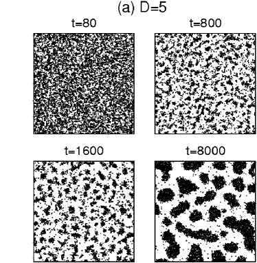
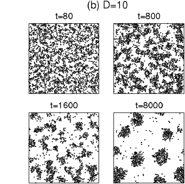
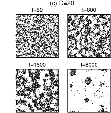
Figure 7: Snapshots of the concentration distribution in cross-section slices (of linear dimensions $L\times L\times\sigma$) centered at the plane $z=D/2$ of the films. We show pictures for (a) $D=5$, (b) $D=10$, and (c) $D=20$. The A-particles are marked black, while the B-particles are not shown. Note that $L=128$ for $D=5$, but $L=64$ for $D=10,20$.

Thus, Fig. 6 already provides evidence of the simultaneous presence of surface enrichment layers and lateral phase separation. A clear picture of lateral phase separation is obtained if we examine the concentration distribution in slices (of width $\sigma$) centered at the $L\times L$ mid-plane at $z=D/2$ (see Fig. 7). These pictures resemble snapshot pictures of 2-$d$ spinodal decomposition, though for an off-critical composition. Of course, the concentration is conserved in a strictly 2-$d$ system, whereas the concentration is not conserved in the shown $L\times L\times\sigma$ slice. As a matter of fact, it decreases systematically with increasing time, due to the progressive formation of A-rich surface enrichment layers. This is particularly evident in the late-time snapshots ($t=8000$) for $D=10$ and $D=20$, respectively.

In order to quantitatively characterize the lateral phase separation, we introduce the layer-wise correlation function:

$$C(\rho,z,t)=\langle\psi(0,z,t)\psi(\vec{\rho},z,t)\rangle-\langle\psi(0,z,t)\rangle\langle\psi(\vec{\rho},z,t)\rangle.$$ (20)

We also define a layer-wise length scale $\ell(z,t)$ from the decay of this function with lateral distance $\rho$:

$$C(\rho=\ell,z,t)=\frac{1}{2}C(0,z,t)\quad.$$ (21)

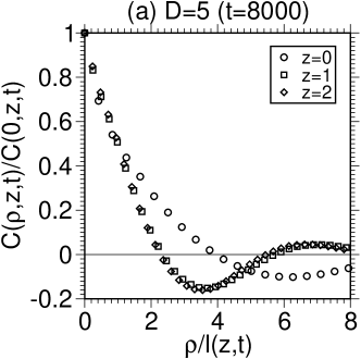
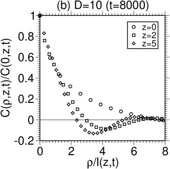
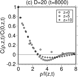
Figure 8: Plot of normalized correlation function $C(\rho,z,t)/C(0,z,t)$ vs. $\rho/\ell(z,t)$ at $t=8000$ for (a) $D=5$, (b) $D=10$, and (c) $D=20$. We show data for several values of $z$ (distance from the left wall), as indicated in the figure. The time $t=8000$ is chosen such that it corresponds to the later stages of coarsening.

In Fig. 8, we plot the scaled layer-wise correlation function, $C(\rho,z,t)/C(0,z,t)$ vs. $\rho/\ell(z,t)$ at $t=8000$, for $D=5,10,20$ and different values of $z$. The surface ($z=0$) is strongly enriched in the preferred component A – see Fig. 4 and Fig. 5. The corresponding correlation function measures small fluctuations about a strongly off-critical background. The correlation functions for the inner regions of the film do not scale either. (If there were scaling, all the data sets in Figs. 8a-c would superimpose, as they do when similar plots are made in studies of bulk spinodal decomposition.) This is because the correlation function is a function of the off-criticality op87 ; sp88 , and different values of $z$ are characterized by different average compositions – see the depth profiles for $t=8000$ in Fig. 4b (for $D=5$) and Fig. 4d (for $D=10$).

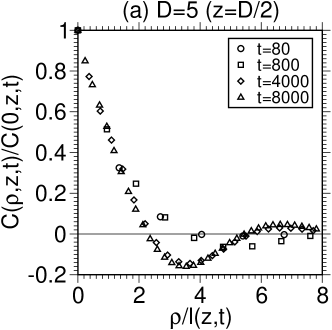
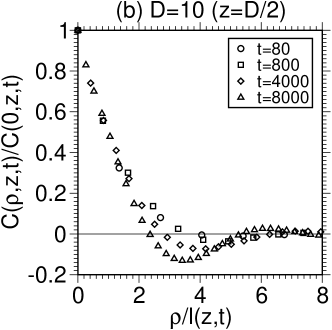
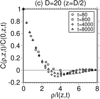
Figure 9: Plot of normalized correlation function $C(\rho,z,t)/C(0,z,t)$ vs. $\rho/\ell(z,t)$ for $z=D/2$, and (a) $D=5$, (b) $D=10$, and (c) $D=20$. We show data for times $t=80,800,4000,8000$ in all cases, as indicated by the different symbols.

In Fig. 9, we show the scaled correlation function in the film center for $D=5,10,20$ at different times. Again, there is no scaling of the data sets. This lack of scaling is expected, however, since the average volume fraction of A in the central region changes with time – see Fig. 4. For the case of $D=5$, there is a reasonable superposition of the curves for $t=4000$ and $t=8000$. This is consistent with the observation that the average concentration at the center remains approximately unchanged over this time-regime – see Fig. 4b. In the asymptotic regime, the system evolves via the lateral coarsening of columnar domains. Therefore, we expect the depth profiles $\psi_{\rm av}(z,t)$ vs. $z$ (as in Fig. 4) to become independent of time at sufficiently large times. In this regime, we will recover dynamical scaling for the layer-wise correlation functions.

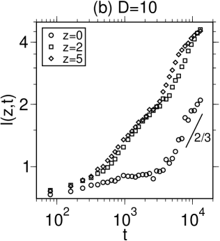
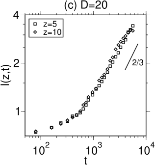
Figure 10: Time-dependence of layer-wise length scale $\ell(z,t)$, plotted on a log-log scale. We show data for different values of $z$, and (a) $D=5$, (b) $D=10$, (c) $D=20$. The straight lines have a slope of 2/3.

In Fig. 10, we plot the layer-wise length scale [$\ell(z,t)$ vs. $t$] for $D=5,10,20$ on a log-log plot, in order to check for possible power laws. At early times, no well-defined power law can be identified at all. This is not surprising as one does not expect a universal growth law to apply when the length scale is of the same order as the inter-particle distance. The gradual increase of the slope of $d[\ln\ell(t)]/d(\ln t)$ is consistent with data from experimental and simulational studies of spinodal decomposition in the bulk 21 ; 22 ; 23 ; 24 ; 25 ; 46 ; 47 ; 48 ; 49 ; 50 . Surprisingly, at later times, the MD data appear to be compatible with a power law with an effective exponent $\simeq 2/3$. We do not see evidence for any of the other growth laws discussed in the context of fluids (see Sec. IIB) over an extended period of time. One might have expected that the LS evaporation-condensation mechanism or the droplet diffusion-coagulation mechanism would dominate over some time-range, but this is not the case. As regards the Siggia tube-coarsening mechanism, the interconnected domain structures break up so early that hydrodynamic mechanisms can hardly become operative.

It would be premature to claim that the log-log plots in Fig. 10 are evidence that the inertial mechanism [Eq. (5)] has been seen. According to theory, this mechanism should be visible only if the length scale $\ell(t)\gg\ell_{\rm in}=\eta^{2}/(n\gamma_{\rm AB})$. Fortunately, the material parameters which determine $\ell_{\rm in}$ are known for our model, as emphasized in Sec. III. Putting the numbers in, we estimate that $\ell_{\rm in}\sim O(10^{2})$! Such large values of $\ell_{\rm in}$ are compatible with studies of the late stages of domain growth in $d=3$ using the lattice Boltzmann method 53 .

One might then conclude that the effective power law $\ell(t)\propto t^{2/3}$ seen in Fig. 10 is only a transient phenomenon, and the power laws that are expected in this case (see Sec. IIB) will come into play at later times. An alternative possibility is that novel growth laws arise due to the interplay of wetting kinetics and lateral phase separation in the “bulk” of the film. However, we note that our results have a striking qualitative similarity to the Brownian-dynamics results of Farrell and Valls 50 . These authors studied phase separation in strictly 2-$d$ fluid mixtures, and found a rapid crossover to a power law $\ell(t)\propto t^{\phi}$ with $\phi\simeq 2/3$.

Obviously, more work with both simulations and theory is needed to resolve the nature of applicable growth laws. However, this cannot be done by simply running our simulations longer. This is because the condition $\ell(z,t)\ll L$ is needed to ensure that finite-size effects in the lateral direction are negligible. Further, the condition $\ell(z,t)\ll L$ is also needed to provide a reasonable self-averaging of $C(\rho,z,t)$ [defined in Eq. (20)]. One can divide the system laterally into independent blocks of linear size $\ell(z,t)$ to judge the error in the estimation of $C(\rho,z,t)$. Therefore, the relative error is less for $D=5$ (where $L=128$) than for $D=10$ and 20 (where $L=64$), and it increases when $\ell(z,t)$ increases. Thus, the irregularities in $\ell(z,t)$ for $D=10,20$ when $t\geq 1000$ are probably due to insufficient statistics (as only three independent runs were made).

V Summary and Discussion

Let us conclude this paper with a summary and discussion of our results. Here, we have presented comprehensive results from molecular dynamics (MD) simulations of surface-directed spinodal decomposition (SDSD). We have used a simple model system, namely a symmetric binary Lennard-Jones (LJ) mixture, confined between identical flat and structureless parallel walls which preferentially attract the A-particles. Only very thin films are accessible – the distance between the origins of the wall potentials was $(D+1)=6,11,21$ in units of the LJ parameter. Further, the finite size of the lateral linear dimension $L$ ($L=128$ for $D=5$, and $L=64$ for $D=10,20$) constrains our work to the early and intermediate stages of domain growth. In this regime, the characteristic length scale of lateral phase separation $\ell(z,t)$ has grown by approximately one decade. Note that we have also restricted attention to deep quenches, much below the critical temperature of phase separation, but above the triple-point temperature, so crystallization is not an issue in our study. At the chosen temperature ($T=1.1$, i.e., $T/T_{\rm c}\simeq 0.67$), the bulk phase separation occurs between almost pure A and B fluids. The interfaces are locally sharp (with a correlation length $\xi\sim 1$), and the time-scale for structural relaxation in the fluids is manageable for MD work. The shear viscosity has been estimated previously 37 to be $\eta\simeq 7$ at $T=1.1$, in the standard LJ units. Thus, the advantages of the present approach are as follows: (a) all material parameters of the model are explicitly known; (b) at small scales, a qualitatively reasonable description of fluid structure is ensured; and (c) long-range hydrodynamic interactions (resulting from the conservation laws in fluid dynamics) are automatically included, although only a short-range LJ potential is chosen to model the interaction among the point particles.

We use this model to elucidate all the main characteristics of SDSD. The surfaces become the origin of SDSD waves, which consist of alternating enrichment and depletion layers of the preferred component A. These waves coalesce in the central region of the film, giving rise to a layered structure – see the $t=800$ profile in Fig. 4b and the $t=4000$ profile in Fig. 4d. This layered state subsequently breaks up into a columnar structure that coarsens laterally – see the cross-sections in Figs. 6 and 7. Therefore, the local concentration of A-particles at the walls grows rapidly at first, resulting in rather large values at early times, followed by a decrease at later times (Fig. 5).

In the initial stages of phase separation, domain growth in the film interior resembles spinodal decomposition in bulk mixtures, where a bicontinuous percolating structure forms at compositions near the critical concentration. During this stage, $\ell(z,t)$ grows only rather slowly (Fig. 10). In this regime, the concentration of A in the film center decreases, due to the growth in thickness of the surface enrichment layers. Therefore, the percolating structure breaks up into separated A-rich droplets which have a cylindrical shape, with height of order $D$ in the $z$-direction and radius of order $\ell(z,t)$. However, these droplets are connected through the A-rich enrichment layers at the walls. The observation that, in this droplet growth stage, the local concentration at the surface decreases can be understood as follows. For the chosen parameters, the B-rich phase exhibits incomplete wetting of A at the walls – for complete wetting, no overshoot of $\psi_{\rm av}(z=0,t)$ vs. $t$ would be expected in Fig. 5. A remarkable feature of our results is that domain growth is compatible with the inertial growth law, $\ell(t)\propto t^{2/3}$, during the droplet growth stage (Fig. 10). This is reminiscent of studies 50 of phase separation in strictly 2-$d$ fluids, where Langevin equations including hydrodynamic interactions were simulated.

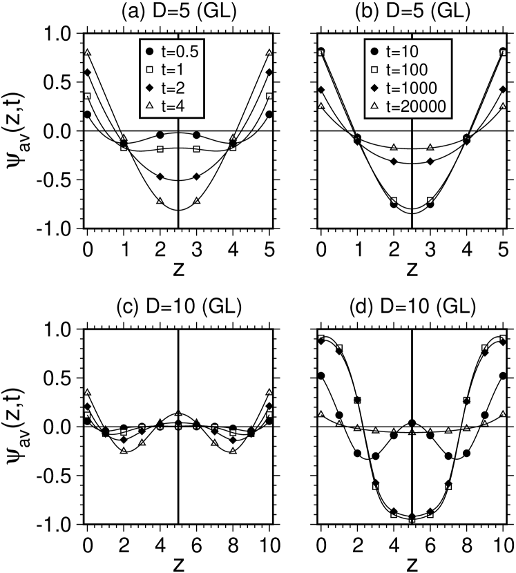
Figure 11: Laterally averaged order parameter profiles, $\psi_{\rm av}(z,t)$ vs. $z$, obtained from the GL simulations described in Sec. II.C 40 . The GL data was obtained as an average over 5 independent runs with $L=256$. We show data for films of thickness (a) $D=5$ at early times ($t=0.5,1,2,4$); (b) $D=5$ at late times ($t=10,100,1000,20000$); (c) $D=10$ at early times ($t=0.5,1,2,4$); (d) $D=10$ at late times ($t=10,100,1000,20000$). The symbol usage is the same for (a),(c) as well as for (b),(d).

It is clear that an extension of the brute force MD approach to much larger linear dimensions (needed at later times) requires prohibitively large amounts of computer time. On the other hand, our MD study does reach mesoscopic length scales, which are significantly larger than inter-particle distances. This suggests that our MD study should be supplemented by Langevin studies of the Ginzburg-Landau (GL) models described in Sec. II.C, so as to enable a simulation extending from microscopic to macroscopic scales. Let us briefly discuss a comparison for the early stages of SDSD in thin films, where the hydrodynamic interactions can be disregarded. Figure 11 is analogous to Fig. 4, but is taken from a GL simulation of model B with appropriate boundary conditions 40 . The details of this simulation are discussed at the end of Sec. II.C. The qualitative similarity of the evolution of the depth profiles in Figs. 4 and 11 is striking. For the GL simulations, the spatial degrees of freedom were rather coarsely discretized (with $\Delta x=1$), and hence the small-scale structure close to the walls cannot be resolved. Apart from this difference, the GL profiles are in good agreement with those obtained from the MD simulation for short times, if we equate the time units as $t_{\rm GL}\simeq 160~{}t_{\rm MD}$. Recall that the natural time-scale in fluids is given in terms of the structural relaxation time 103 , and the latter is of the same order as the shear viscosity, which is $\eta\simeq 7$ LJ units in this case. Since the MD time unit $t_{\rm MD}\equiv t_{0}\simeq 1/\sqrt{48}\simeq 1/7$ LJ units, we conclude that the natural fluid time-scale is about 50 MD time units.

The qualitative behavior of the GL results 40 (formation of surface enrichment layers and a metastable layered state $\rightarrow$ break up due to lateral phase separation $\rightarrow$ coarsening of columnar structures) is similar to the results of the present MD study. However, in quantitative respects, the intermediate stages of coarsening are rather different for the GL model. When the layered state breaks up into a laterally inhomogeneous state in the GL model, one often encounters a period of time where $\ell$ stays roughly constant, or even decreases. We do not observe such a transient behavior in the MD runs – as a matter of fact, the layered state does not survive for any appreciable period of time. Further, asymptotic domain growth in the GL model is compatible with an $\ell(t)\propto t^{1/3}$ law, as predicted by the Lifshitz-Slyozov theory. On the other hand, our MD results are consistent with a growth law $\ell(t)\propto t^{2/3}$. Clearly, a GL study of SDSD in thin films, which incorporates hydrodynamic interactions, would be very desirable. Further, a detailed comparison of the present MD results with corresponding lattice Boltzmann studies should be worthwhile, but is left to future studies. Finally, we hope that the present work will further stimulate experimental studies of phase separation in thin films.

Acknowledgments: We thank the Deutsche Forschungsgemeinschaft (DFG) for support via grant No Bi 314/18-2 (SKD), the Emmy Noether Program (JH), and grant SFB 625/A3 (SP).

Figure 2: Schematic phase diagrams (a,b) and corresponding states (c) of a symmetric AB mixture in a thin film of thickness $D$. The film is symmetric, viz., both walls attract the A-particles with the same strength. We emphasize that the wetting transition only occurs in the limit $D\rightarrow\infty$. For finite $D$, the transition of the walls from nonwet (or partially wet) to wet (or completely wet) is rounded into a smooth gradual change. This transition is of second order in (a), while (b) refers to a first-order wetting transition. In (b), a prewetting transition line exists in the one-phase region, with one end being a prewetting critical point at high temperatures. The other end of this line is at the wetting transition temperature $T_{\rm w}$, at the coexistence curve that separates the two-phase region from the one-phase region. Note that the critical concentration of a symmetric binary mixture is $x^{\rm crit}_{\rm A}=0.5$ in the bulk, but is shifted to a larger value $x_{\rm A}$ in the thin film. Further, the critical temperature of the film typically is lower than in the bulk, $T_{\rm c}(D)<T_{\rm c}(\infty)=T_{\rm c}$. For the case of first-order wetting and large enough $D$, a thin-film analog of the prewetting transition exists, as evidenced by the thin-film critical point at the left side of the phase diagram. When the thin enrichment layer segregation meets the lateral segregation of the “thick” film, a thin-film triple point occurs at a temperature close to $T_{\rm w}$. For thin films, this triple point and the left critical point may merge and annihilate each other, and then the corresponding phase diagram is similar to that in (a). In (c), we provide schematic pictures of the thin-film states in the case of lateral phase separation.

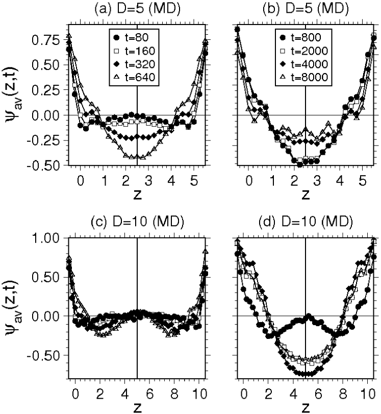
Figure 4: Laterally averaged order parameter profiles, $\psi_{\rm av}(z,t)$ vs. $z$, for films of thickness (a) $D=5$ at early times ($t=80,160,320,640$); (b) $D=5$ at late times ($t=800,2000,4000,8000$); (c) $D=10$ at early times ($t=80,160,320,640$); (d) $D=10$ at late times ($t=800,2000,4000,8000$). The symbol usage is the same for (a),(c) as well as for (b),(d).

References

- (1) Y. Champion and H. J. Fecht (eds.), Nano–Architectured and Nano–Structured Materials (Wiley–VCH, Weinheim, 2004).
- (2) E. L. Wolf, Nanophysics and Nanotechnology (Wiley–VCH, Weinheim, 2004).
- (3) C. N. R. Rao, A. Müller, and A. K. Cheetham (eds.), The Chemistry of Nanomaterials (Wiley–VCH, Weinheim, 2004).
- (4) R. Kelsall, I. W. Hamley, and M. Geoghegan (eds.), Nanoscale Science and Technology (Wiley-VCH, Weinheim, 2005).
- (5) G. Decker and J. B. Schlenoff (eds.), Multilayer Thin Films: Sequential Assembly of Nanocomposite Materials (Wiley–VCH, Weinheim, 2002).
- (6) H. Watarai, Interfacial Nanochemistry: Molecular Science and Engineering at Liquid-Liquid Interfaces (Springer, Berlin, 2005).
- (7) A. Marrion (ed.), The Chemistry and Physics of Coatings (Springer, Berlin, 2004).
- (8) J. Charvolin, J.-F. Joanny, and J. Zinn-Justin (eds.), Liquids at Interfaces (North-Holland, Amsterdam, 1990).
- (9) S. Granick (ed.), Polymers in Confined Environments, Advances in Polymer Science, Vol. 138 (Springer, Berlin, 1999).
- (10) B. Dünweg, D. P. Landau, and A. I. Milchev (eds.), Computer Simulations of Surfaces and Interfaces (Kluwer Acad. Publ., Dordrecht, 2003).
- (11) H. J. Butt, K. Graf, and M. Kappl, Physics and Chemistry of Interfaces (Wiley-VCH, Weinheim, 2003).
- (12) P. G. de Gennes, Rev. Mod. Phys. 57, 827 (1985).
- (13) D. E. Sullivan and M. M. T. da Gama, in C. A. Croxton (ed.), Fluid Interfacial Phenomena (Wiley, New York, 1986), chap. 2.
- (14) S. Dietrich, in C. Domb and J. L. Lebowitz (eds.), Phase Transitions and Critical Phenomena, Vol. 12 (Academic Press, London, 1988), chap. 1.
- (15) M. Schick, in Ref. 8 , p. 415.
- (16) G. Forgacs, R. Lipowsky, and T. M. Nieuwenhuizen, in C. Domb and J. L. Lebowitz (eds.), Phase Transitions and Critical Phenomena, Vol. 14 (Academic Press, London, 1991), chap. 2.
- (17) K. Binder, in D. G. Pettifor (ed.), Cohesion and Structure of Surfaces (Elsevier Science, Amsterdam, 1995), p. 121.
- (18) D. Bonn and D. Ross, Rep. Prog. Phys. 64, 1085 (2001).
- (19) M. M. Telo da Gama, in Ref. 10 , p. 239.
- (20) K. Binder, D. P. Landau, and M. Müller, J. Stat. Phys. 110, 1411 (2003).
- (21) J. D. Gunton, M. San Miguel, and P. S. Sahni, in C. Domb and J. L. Lebowitz (eds.), Phase Transitions and Critical Phenomena, Vol. 8 (Academic Press, London, 1983), p. 267.
- (22) S. Komura and H. Furukawa (eds.), Dynamics of Ordering Processes in Condensed Matter (Plenum Press, New York, 1988).
- (23) A. J. Bray, Adv. Phys. 43, 357 (1994).
- (24) K. Binder and P. Fratzl, in G. Kostorz (ed.), Phase Transformations in Materials (Wiley-VCH, Weinheim, 2001), p. 409.
- (25) A. Onuki, Phase Transition Dynamics (Cambridge Univ. Press, Cambridge, 2002).
- (26) S. Dattagupta and S. Puri, Dissipative Phenomena in Condensed Matter: Some Applications (Springer, Berlin, in press).
- (27) R. A. L. Jones, L. J. Norton, E. J. Kramer, F. S. Bates, and P. Wiltzius, Phys. Rev. Lett. 66, 1326 (1991).
- (28) S. Puri and K. Binder, Phys. Rev. A 46, R4487 (1992); Phys. Rev. E 49, 5259 (1994).
- (29) G. Brown and A. Chakrabarti, Phys. Rev. A 46, 4829 (1992).
- (30) G. Krausch, Mater. Sci. Eng. Rep. R 14, 1 (1995).
- (31) S. Puri and H. L. Frisch, J. Phys.: Condens. Matter 9, 2109 (1997).
- (32) K. Binder, J. Non–Equ. Thermodyn. 23, 1 (1998).
- (33) S. Puri and K. Binder, Phys. Rev. Lett. 86, 1797 (2001); Phys. Rev. E 66, 061602 (2002).
- (34) J. M. Geoghegan and G. Krausch, Prog. Polym. Sci. 28, 261 (2003).
- (35) S. Puri, J. Phys.: Condens. Matter 17, R101 (2005).
- (36) S.K. Das, S. Puri, J. Horbach, and K. Binder, Phys. Rev. Lett. 96, 016107 (2006).
- (37) S. K. Das, J. Horbach, and K. Binder, J. Chem. Phys. 119, 1547 (2003).
- (38) S. K. Das, J. Horbach, and K. Binder, Phase Transitions 77, 823 (2004).
- (39) K. Binder, S. K. Das, J. Horbach, M. Müller, R. Vink, and P. Virnau, in S. Attinger and P. Koumoutsakos (eds.), Multiscale Modelling and Simulation (Springer, Berlin, 2004), p. 169.
- (40) S. Puri and K. Binder, J. Stat. Phys. 77, 145 (1994).
- (41) S. K. Das, S. Puri, J. Horbach, and K. Binder, Phys. Rev. E 72, 061603 (2005).
- (42) T. Kawasaki and T. Ohta, Prog. Theoret. Phys. 59, 362 (1978).
- (43) E. Siggia, Phys. Rev. A 20, 595 (1979).
- (44) M. San Miguel, M. Grant, and J. D. Gunton, Phys. Rev. A 31, 1001 (1985).
- (45) H. Furukawa, Phys. Rev. A 31, 1103 (1985); ibid 36, 2288 (1987).
- (46) H. Furukawa, Physica A 204, 237 (1994).
- (47) S. Puri and B. Dünweg, Phys. Rev. A 45, R6977 (1992).
- (48) T. Koga and K. Kawasaki, Phys. Rev. A 44, R817 (1991); Physica A 196, 389 (1993).
- (49) A. Shinozaki and Y. Oono, Phys. Rev. E 48, 2622 (1993).
- (50) T. Koga, K. Kawasaki, M. Takenaka, and T. Hashimoto, Physica A 198, 473 (1993); T. Koga, H. Jinnai and T. Hashimoto, Physica A 263, 369 (1999).
- (51) J. E. Farrell and O. T. Valls, Phys. Rev. B 40, 7027 (1989); Phys. Rev. B 42, 2353 (1990); Phys. Rev. B 43, 630 (1991).
- (52) V. M. Kendon, J.-C. Desplat, P. Bladon, and M. E. Cates, Phys. Rev. Lett. 83, 576 (1999); V. M. Kendon, M. E. Cates, I. Pagonabarraga, J.-C. Desplat, and P. Bladon, J. Fluid Mech. 440, 147 (2001).
- (53) I. Pagonabarraga, A. J. Wagner, and M. E. Cates, J. Stat. Phys. 107, 39 (2002).
- (54) F. J. Alexander, S. Chen, and D. W. Grunau, Phys. Rev. B 48, 634 (1993).
- (55) T. Lookman, Y. Wu, F. J. Alexander, and S. Chen, Phys. Rev. E 53, 5513 (1996).
- (56) C. Appert, J. F. Olson, D. H. Rothman, and S. Zaleski, J. Stat. Phys. 81, 181 (1995).
- (57) S. Bastea and J. L. Lebowitz, Phys. Rev. Lett. 78, 3499 (1997).
- (58) S. I. Jury, P. Bladon, S. Krishna, and M. E. Cates, Phys. Rev. E 59, R2535 (1999).
- (59) A. J. Briant, P. Papatzacos, and J. M. Yeomans, Philos. Trans. R. Soc. London, Ser. A 360, 485 (2002).
- (60) A. Dupuis and J. M. Yeomans, Langmuir 21, 2624 (2005); Future Generation Computer System 20, 993 (2004); Pramana 64, 1019 (2005).
- (61) A. J. Wagner and J. M. Yeomans, Phys. Rev. Lett. 80, 1429 (1998).
- (62) H. Furukawa, Phys. Rev. E 61, 1423 (2000).
- (63) A. J. Wagner and M. E. Cates, Europhys. Lett. 56, 556 (2001).
- (64) M. Laradji, S. Toxvaerd, and O. G. Mouritsen, Phys. Rev. Lett. 77, 2253 (1996).
- (65) E. Velasco and S. Toxvaerd, Phys. Rev. Lett. 71, 388 (1993).
- (66) P. Ossadnik, M. F. Gyure, H. E. Stanley, and S. Glotzer, Phys. Rev. Lett. 72, 2498 (1994).
- (67) W.-J. Ma, P. Keblinski, A. Maritan, J. Koplik, and J.R. Banavar, Phys. Rev. E 48, R2362 (1993).
- (68) S. Toxvaerd, Phys. Rev. Lett. 83, 5318 (1999).
- (69) K. Binder, in C. Domb and J. L. Lebowitz (eds.), Phase Transitions and Critical Phenomena, Vol. 8 (Academic Press, London, 1983), p. 1.
- (70) M. E. Fisher and H. Nakanishi, J. Chem. Phys. 75, 5857 (1981); H. Nakanishi and M. E. Fisher, J. Chem. Phys. 78, 3279 (1983).
- (71) R. Evans and P. Tarazona, Phys. Rev. Lett. 52, 557 (1984).
- (72) D. Nicolaides and R. Evans, Phys. Rev. B 39, 9336 (1989).
- (73) R. Evans, J. Phys.: Condens. Matter 2, 8989 (1990).
- (74) K. Binder and D. P. Landau, J. Chem. Phys. 96, 1444 (1992).
- (75) K. Binder, Ann. Rev. Phys. Chem. 43, 33 (1992).
- (76) Y. Rouault, J. Baschnagel, and K. Binder, J. Stat. Phys. 80, 1009 (1995).
- (77) T. Flebbe, B. Dünweg, and K. Binder, J. Phys. II (France) 6, 667 (1996).
- (78) K. Binder, P. Nielaba, and V. Pereyra, Z. Phys. B 104, 81 (1997).
- (79) M. Müller and K. Binder, Macromolecules 31, 8323 (1998).
- (80) M. E. Fisher, Rev. Mod. Phys. 46, 597 (1974).
- (81) K. Binder and E. Luitjen, Phys. Rep. 344, 179 (2001).
- (82) L. D. Gelb, K. E. Gubbins, R. Radhakrishnan, and M. Slivinska-Bartkowiak, Rep. Prog. Phys. 62, 1573 (1999).
- (83) D. M. Kroll and G. Gompper, Phys. Rev. B 39, 433 (1989).
- (84) J. O. Indekeu, Int. J. Mod. Phys. 138, 309 (1994).
- (85) J. Drelich, Colloids Surf. A 116, 43 (1996).
- (86) T. Getta and S. Dietrich, Phys. Rev. E 57, 655 (1998); C. Bauer and S. Dietrich, Eur. Phys. J. B 10, 767 (1999).
- (87) A. Milchev and K. Binder, J. Chem. Phys. 114, 8610 (2001).
- (88) L. G. MacDowell, M. Müller, and K. Binder, Coll. Surf. A 206, 277 (2002).
- (89) I. M. Lifshitz and V. V. Slyozov, J. Phys. Chem. Solids 19, 35 (1961).
- (90) K. Binder and D. Stauffer, Phys. Rev. Lett. 33, 1006 (1974); K. Binder, Phys. Rev. B 15, 4425 (1977).
- (91) H. W. Diehl, in C. Domb and J. L. Lebowitz (eds.), Phase Transitions and Critical Phenomena, Vol. 10 (Academic Press, New York, 1986), p. 75.
- (92) P. C. Hohenberg and B. I. Halperin, Rev. Mod. Phys. 49, 435 (1977).
- (93) S. Puri and Y. Oono, J. Phys. A 21, L755 (1988).
- (94) K. Binder and H. L. Frisch, Z. Phys. B 84, 403 (1991).
- (95) K. Binder and G. Ciccotti (eds.), Monte Carlo and Molecular Dynamics of Condensed Matter Systems (Italian Physical Society, Bologna, 1996).
- (96) D. C. Rapaport, The Art of Molecular Dynamics Simulation (Cambridge University Press, Cambridge, 1995).
- (97) K. Binder, J. Horbach, W. Kob, W. Paul, and F. Varnik, J. Phys.: Condens. Matter 16, S429 (2004).
- (98) F. Varnik and K. Binder, J. Chem. Phys. 117, 6336 (2002).
- (99) A. Milchev, D. W. Heermann, and K. Binder, Z. Phys. B 63, 521 (1986).
- (100) Y. Oono and S. Puri, Phys. Rev. Lett. 58, 836 (1987); Phys. Rev. A 38, 434 (1988); S. Puri and Y. Oono, Phys. Rev. A 38, 1542 (1988).
- (101) S. Puri, Phys. Lett. A 134, 205 (1988).