The breaking of quantum double symmetries by defect condensation
Abstract
In this paper, we study the phenomenon of Hopf or more specifically quantum double symmetry breaking. We devise a criterion for this type of symmetry breaking which is more general than the one originally proposed in [1, 2], and therefore extends the number of possible breaking patterns that can be described consistently. We start by recalling why the extended symmetry notion of quantum double algebras is an optimal tool when analyzing a wide variety of two dimensional physical systems including quantum fluids, crystals and liquid crystals. The power of this approach stems from the fact that one may characterize both ordinary and topological modes as representations of a single (generally non-Abelian) Hopf symmetry. In principle a full classification of defect mediated as well as ordinary symmetry breaking patterns and subsequent confinement phenomena can be given. The formalism applies equally well to systems exhibiting global, local, internal and/or external (i.e. spatial) symmetries. The subtle differences in interpretation for the various situations are pointed out. We show that the Hopf symmetry breaking formalism reproduces the known results for ordinary (electric) condensates, and we derive formulae for defect (magnetic) condensates which also involve the phenomenon of symmetry restoration. These results are applied in two papers which will be published in parallel [3, 4].
keywords:
Quantum doubles , liquid crystals , phase transitions , defect condensates , Hopf algebras , topological phasesPACS:
02.20.Uw , 64.60.-i , 61.30.-v , 61.72.-y, ††thanks: Present address: Physics Department, Princeton University, Jadwin Hall, Princeton, NJ 08544, United States
1 Introduction and motivations
In recent years it has become clear that in the setting of two-dimensional (quantum) physics, the notion of quantum double algebras or quantum groups plays an important role. One of the main reasons is that these extended symmetry concepts allow for the treatment of topological and ordinary quantum numbers on equal footing. This means that the representation theory of the underlying - hidden - Hopf algebra labels both the topological defects and the ordinary excitations. This is also the case in non-Abelian situations where the mutual dependence of these dual quantum numbers would otherwise be untractable. Moreover, as the Hopf algebras involved turn out to be quasi-triangular they are naturally endowed with a -matrix which describes the topological interactions between the various excitations in the medium of interest [5, 6]. This theory has found interesting applications in the domain of Quantum Hall liquids [7, 8, 9, 10, 11], exotic phases in crystals and liquid crystals [3], as well as 2-dimensional gravity [12]. It also appears to furnish the appropriate language in the field of topological quantum computation [13, 14, 15, 16].
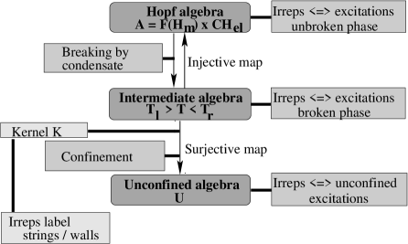
Once this (hidden) extended symmetry was identified, the authors of [1, 2] studied the breaking the Hopf symmetry by assuming the formation of condensates, respectively of ordinary (which we call electric), defect (magnetic), or mixed (dyonic) type. As was to be expected, the ordinary condensates reproduce the conventional theory of symmetry breaking, though the analysis of confinement of topological degrees of freedom, using the braid group, is not standard. In [1, 2] it was shown that when considering Hopf symmetry breaking, the usual formalism of symmetry breaking had to be extended with significant novel ingredients. One assumes the condensate to be represented by a fixed vector in some nontrivial representation of the Hopf algebra . This leads to the definition of an intermediate algebra as the suitably defined stabilizer subalgebra of the condensate. The complication that arises at this level is that certain representations of may braid nontrivially with the condensate, which in turn means that the condensate cannot be single valued around a particle belonging to such a representation. If this happens to be the case, it implies that such particles (representations) necessarily are confined. The effective low energy theory of the non-confined degrees of freedom is then characterized by yet a smaller algebra called . So the breaking of Hopf symmetries involves three algebras: the unbroken algebra , the intermediate algebra , and the unconfined algebra .
In this paper we show that the assumptions made about the structure of the intermediate residual symmetry algebra in [1, 2] can be relaxed. This leads to a new definition of the residual symmetry algebra which contains as a subalgebra, which means that the residual phase may have a richer spectrum. We will discuss the new criterion in some detail and point out its importance.
We conclude by deriving general formulae for and for the case of electric and defect condensates, in phases whose corresponding Hopf algebra is what we call a modified quantum double , where and are finite groups. is the magnetic group, i.e. the defect group. is the electric group, or the residual symmetry group1. We know what to expect for electric condensates, and for that case our method reproduces the known results. The problem of defect condensates is more interesting, and provided the main motivation for this work. In this paper we focus on the basic structure and the more formal aspects of the symmetry breaking analysis and we mainly present general results, involving both confinement and liberation phenomena. In two separate papers we give detailed applications of these results: one paper on defect mediated melting [4] (which discusses also the phenomenon of symmetry restoration), and another on the classification of defect condensates in non-abelian nematic crystals [3].
The starting point in this paper will be situations where a continuous internal or external (space) symmetry is broken to a possibly non-abelian, discrete subgroup . This may happen through some Higgs mechanism in which case we speak of discrete gauge theories [17], or by forming some liquid crystal for example. Topological (line) defects can then be labelled by the elements of the discrete residual symmetry group2 . Familiar examples of such defects are dislocations, disclinations, vortices, flux-tubes etc. Such a theory has a (hidden) Hopf symmetry corresponding to the so called quantum double of . This Hopf symmetry is an extension of the usual group symmetry3. The elements of are denoted by , where is some function on the group , and some element of the group algebra of (later on we will omit the sign). A basis for the space of functions on a discrete group is a set of delta functions which project on each group element. We denote these projectors by , these are just delta functions () defined by: }. The element is basically a measurement operator (projecting on a subspace), while involves a symmetry operation. In other words, if we denote the elements of the group by , where labels the group elements, we can write
where the and are complex numbers. This follows from the fact that the span , and the span the group algebra of , which we denote by . An alternate notation for is , which shows that it is a combination of and .
The multiplication of two elements of is defined by
| (1) |
Note that the multiplication on the group part is just the ordinary group multiplication, but the multiplication of the functions is not just pointwise but twisted by a conjugation. This is a nontrivial feature which implies that the product is not a simple tensor product. There are two structures on a Hopf algebra of special interest to our purposes (for an introduction to Hopf algebras, see for example [18]). One is the so called counit which turns out to be of particular relevance in the present context. is an algebra morphism from the Hopf algebra to , defined through . The other structure we wish to mention is the antipode which is a kind of inverse needed to introduce conjugate or antiparticle representations. is an algebra antimorphism from to , which satisfies . A quantum double is further endowed with an invertible element which implements the braiding of representations. It encodes the topological interactions and in particular the possible exotic “quantum statistics properties” of the excitations in the system.
The sectors of the theory, or the physical excitations for that matter, can be labelled by the irreducible representations of . These are denoted as , where the label denotes the conjugacy class to which the topological (magnetic) charge of the excitation belongs, whereas denotes a representation of the centralizer group of a chosen preferred element of . fixes the “ordinary” or electric charge. Clearly, describes in general a mixed electric and magnetic, usually called dyonic, excitation. Pure defects or ordinary excitations correspond to the special cases where one of the two labels becomes trivial. We denote the carrier space on which acts as . The Hopf algebra structure requires a well defined comultiplication which ensures the existence of well defined fusion or tensor product rules for the representations of the algebra.
The quantum double appears when the defect group , which we call the magnetic group, and the residual symmetry group , which we call the electric group, are the same group . This is often the case, because the magnetic group is equal to , when is connected and simply connected. However, there are cases where and are not equal. For example, if we want to distinguish between chiral and achiral phases, we have to include inversions (or reflections). The inclusion of inversions does not alter the defect group (because the inversions live in a part of that isn’t connected to the identity), but it can alter the electric group. We are thus led to the structure of a modified quantum double , which is a special case of what is called a bicrossproduct4 of the Hopf algebras and . The structures in are very similar to those in , we give them in appendix A. The crucial point is that the electric group acts on the magnetic group, namely a residual symmetry transformation transforms the defects. We denote the action of on by . In the case of , the action is simply conjugation: . To obtain the structures of from those of , one basically replaces all occurrences of by .
2 Breaking, braiding and confinement
In the previous section we mentioned that a Hopf symmetry captures the fusion and braiding properties of excitations of spontaneously broken phases. In particular we mentioned the modified quantum double , which is relevant for a phase with magnetic group and electric group . In this section we will show that this Hopf symmetry description allows for a systematic investigation of phase transitions induced by the condensation of some excitation. Since electric, magnetic and dyonic modes are treated on equal footing, we will unify the study of phase transitions induced by the formation of condensates of all three types of modes.
The use of Hopf symmetries to analyze phase transitions was pioneered by Bais, Schroers and Slingerland [1, 2]. In this article we stay close to their work. An important departure however, is the definition of ”residual symmetry operators”. Based on physical arguments we put forward a new definition, which, though similar, is more general than the previous one.
2.1 Breaking
We want to study the ordered phases arising if a condensate forms, corresponding to a non-vanishing vacuum expectation value of some vector which we denote as in some representation of the Hopf algebra. This vacuum vector breaks the Hopf-symmetry , and just as in the conventional cases of spontaneous symmetry breaking we have to analyze what the residual symmetry algebra is.
The natural criterion to determine the residual symmetry that was proposed in [1, 2] is
| (2) |
where is the representation in which lives. The motivation for this criterion is that an operator is a residual symmetry operator if it acts on as the trivial representation .
This condition was subsequently analyzed in [1, 2], where it was argued that one must impose further restrictions on . Namely, it was imposed that be the maximal Hopf subalgebra of that satisfies the condition (2). This restriction was made under the quite natural physical assumption that one should be able to fuse representations of .
We have taken a closer look at this restriction, and the point we make in this paper is that need not be a Hopf algebra. It turns out that there is no physical reason to require to be Hopf, and in fact lifting that requirement opens up a number of very interesting new possibilities that appear to be essential in describing realistic physical situations. Rather than talking about a single Hopf-algebra we have to distinguish two algebras (not necessarily Hopf) and . One can choose either one and we choose to define the breaking with . is defined as the set of operators in that satisfy
| (3) |
We will explain the physical motivation for this criterion later on. Stated in words: the residual symmetry operators belonging to are operators that cannot distinguish whether a given particle has fused with the condensate or not. Therefore these operators are so to say “blind” to the condensate, and the measurements they are related to are not affected by the presence of the condensate. We note for now that need not be a Hopf algebra, but that it contains the Hopf algebra as a subalgebra. Still, all its elements satisfy , thus the operators in also act as the vacuum representation on .
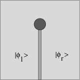
The important difference with the previous analysis of [1, 2], is that, as we have lifted the Hopf algebra requirement on , we will in general no longer have a well defined tensor product for the representations of . At first sight this seems problematic from a physical point of view, but the opposite turns out to be the case, the ambiguity that arises reflects the physical situation perfectly well. Imagine that we bring some localized excitation into the medium, moving it in from the left, then it may well be that the vacuum is not single valued when “moved” around this excitation. If such is the case the excitation will be confined, and we obtain a situation as depicted in Figure 1. The confined particle is connected to a domain wall. The condensate to the right of the wall is in the state , and to the left it is in the state . Thus the question arises where the condensate takes on the original value . When we say the condensate is in the state , and we want to study confined excitations, we must specify whether the state of the condensate is to the far left or the far right of the plane, away from any excitations. We cannot a priori impose that the state of the condensate to the far left and the far right is the same, because then we wouldn’t allow for confined excitations. Choosing to set , i.e. setting the state of the condensate to the far right, gives as intermediate symmetry algebra. Choosing gives us a different intermediate algebra . As mentioned before we’ll work with .
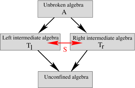
One may now restrict oneself to the unconfined representations and obtain that they form the representations of yet another algebra, the unconfined (Hopf) algebra . Putting it all together we have arrived at the picture in figure 2 for the generic symmetry breaking scheme.
The mathematical structure is appealing and exactly reflects the
subtlety of having to deal with confined particle
representations.
One may show that the maximal Hopf-subalgebra satisfying
the criterion (2) is contained in the
intersection of and :
| (4) |
It is also possible to demonstrate that if is a Hopf algebra then we have necessarily the relation . We will show these and other results later.
In the following sections we motivate the Hopf symmetry breaking formalism by way of examples, and we fully analyze electric and defect condensates starting with phases whose Hopf symmetry is a modified quantum double . The breaking by electric condensates proceeds along familiar lines (i.e. Landau’s theory of phase transitions). However, our arguments are more complete also in these situations, because within our formalism we arrive at a residual symmetry algebra where all defects are still present, and we then find by analyzing which defects are confined, and removing them from the spectrum.
The fact that we reproduce the theory of electric condensates is encouraging. More interesting nontrivial results occur when we analyze defect condensates. Applications of the results of this paper to defect condensates in general classes of nematic liquid crystals [3], and defect mediated melting [4], will be published elsewhere.
Excitations in the broken phase, which has as its symmetry algebra, should form representations of . We must now take a close look at these excitations: some of them turn out to be attached to a domain wall, i.e. their presence would require a half-line singularity in the condensate, and such a wall costs a finite amount of energy per unit length (as we will show later in a simple example). To see this, we must first discuss braiding. It is also useful to discuss the issue of braiding, to point out characteristic differences between phases in which local and global symmetries are broken.
2.2 Braiding
Braiding addresses the question of what happens to a multi-particle state when one particle is adiabatically transported around another. To answer this question one is led to introducing a braid operator, whose properties we briefly recall. We focus our discussion on phases with a Hopf symmetry. We start with some heuristic arguments first involving the braiding of a defect and an ordinary excitation, then the braiding of two defects, and finally that of two ordinary excitations. We will assume throughout that is discrete.
Consider the braiding of an electric mode with a defect in the gauge theory case, because the global case is more subtle. This question goes back to the very definition (or measurement) of the defect [19]. If we have a discrete gauge theory with a defect , then is the “topological charge” of the defect, and it is defined as the path-ordered exponential of the gauge field along a path around the defect:
This phase factor basically corresponds to the change of the wave function (which takes a value in some irreducible representation of the gauge group ) of some particle coupled to the gauge field when it is parallel transported around the defect. The outcome is
| (5) |
So is defined through the condition of a vanishing covariant derivative: .
Thus as an electric mode is transported around the defect, it is acted on by the topological charge defining the defect. We can choose a gauge such that the field is constant everywhere except along a line going “up” from the origin. Then half-braiding already gives , because underneath the defect is constant, i.e. braids trivially with the defect if it passes below the defect. This just shows that this distinction is gauge dependent, because the operator itself is. Indeed, even the path ordered exponential in (5) is not gauge invariant in the nonabelian case, however the conjugacy class to which it belongs is. In a locally invariant theory any physical outcome can only depend on some gauge invariant expression involving this path ordered exponential.
Let us now discuss the braiding of two defects [17, 6]. If we carry a defect counterclockwise around a defect then gets conjugated by and becomes , while gets conjugated to . We can encode this behavior by defining a braid operator . If lives in and in , then is a map from to whose action is defined by (in the local theory this involves adopting some suitable gauge fixing):
| (6) |
The braid operator encodes the braiding properties of the defects.
Note that it braids the defect to the right halfway around the
other defect, it implements a half-braiding or an
interchange. To achieve a full braiding, we have to apply the
monodromy operator which equals .
The equation for the braiding of defects and we have
just discussed applies equally well to the cases of global and
local symmetry breaking.
Finally, it is clear that electric modes braid trivially with each other5:
| (7) |
Before turning to more formal aspects of braiding let us comment on the case of global symmetry. For example in a crystal the defects are defined using a Burgers vector (giving a displacement after circumventing a dislocation) or a Frank vector (specifying a rotation being the deficit angle after one carries a vector around a disclination). The first has to do with translations and the other with discrete rotations, both are elements of the discrete symmetry group of the lattice. The story is thus very similar to the local case. The essence is that the local lattice frame is changed while circumventing the defect (one speaks of “frame dragging”) and that will obviously affect the propagation of local degrees of freedom, whether these are ordinary modes or other defects.
There is also a “continuum approach” to lattice defects where these are considered as singularities in the curvature and torsion of some metric space. In other words, the defects affect the space around them, which will leave its traces if one is to bring a particle around the defect. This idea has been used in crystals, and the resulting geometry is of the Riemann-Cartan type6 where the disclinations and dislocations can be considered as singular nodal lines of curvature and torsion respectively. For an introduction, see [20] and [21]. Clearly this geometrical approach to defects assumes some suitable continuum limit to be taken, which turns the theory into an gauge theory (just like gravity is an gauge theory).
Describing phases with global symmetries in terms of gauge fields leads to the analog of the Aharonov-Bohm effect in global phases. This has been studied in many phases, such as superfluid helium [22], crystals [23], and uniaxial nematic liquid crystals [24] (neglecting diffusion).
So far it is clear that for the global theory, the outcome of braiding is basically the same as in the local case. The frame dragging however is locally measurable and cannot be changed by local gauge transformations. This means that the global theory may admit additional (nonivariant) observables.
We have seen that in basically all situations the action of the braid operator on a two-particle state consisting of a defect and an ordinary (electric) excitation is
| (8) | |||
| (9) |
The beauty of many Hopf algebras - and the quantum double is one of them - is that they are quasitriangular, which means that they are naturally endowed with a universal R-matrix denoted by . is an element of . It encodes the braiding of states of the irreps of : to braid two states, in and in , act with on , and then apply the flip operator . This gives the action of the braid operator :
| (10) |
The operator trivially interchanges any two vectors and around:
| (11) |
The braid (or rather monodromy) operator shows up in invariant physical quantities. For example in the gauge theory case, the expression for the cross section for the nonabelian analogue of Ahoronov-Bohm scattering involving the monodromy operator was given by E. Verlinde [25]:
| (12) |
where is the initial internal wavefunction of the whole system, and the incoming momentum. For example, for the case of an electric mode to the left of a vortex , we have . If the braiding is trivial, i.e. , then there is no scattering.
The question whether this expression for the cross section is also valid in the case of global symmetries, has not been answered conclusively, see for example [26]. As far as the analysis of conceivable ways to break Hopf symmetries, the general theory applies to both situations, but in the actual application there is a precise mathematical difference between phases with local or global symmetries.
2.3 Confinement
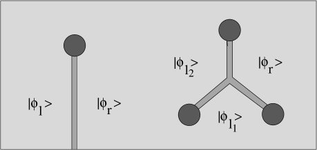
We have already indicated that excitations which braid nontrivially with the vacuum state cannot be strictly local excitations, because the condensate cannot be single valued around them. Such an excitation can only be excited at the price of creating a physical halfline singularity attached to it. One has to create a configuration of a domain wall ending at a defect and therefore we say that such a defect is confined. The fate - such as confinement - of defects in phase transitions where the topology changes was discussed in relation with a particular exact sequence of homotopy mappings in [27]. We will see that the condensate and hence the vacuum vector takes a different value to the left and to the right of the domain wall. And since the domain wall emanating from the excitation costs a finite amount of energy per unit length, we have to conclude that such an excitation will be linearly confined. A finite energy configuration requires another confined excitation on the other end of the wall. We will call a configuration consisting of a number of confined constituents connected by a set of walls, a hadronic composite, in analogy with the hadrons in QCD, being the unconfined composites of confined quarks (see Figure 3). The excitations that braid trivially with the condensate are clearly unconfined, and they can propagate as isolated particles.
To illustrate some of these aspects in more detail, we take a look at the ubiquitous XY-model in two dimensions, and reinterpret the phase transition to the ordered state as an example where confinement plays a role.
Let be the angular variable of the XY model, and the order parameter. The equation that has to satisfy in order to minimize the free energy of the XY model is Laplace’s equation in two dimensions:
| (13) |
There are point singular solutions of (13) that correspond to a defect of charge centered at . There are also other singular solutions of (13), in which the singularity is a half-line. They are labelled by a and a vector and the corresponding solution is given by
| (14) |
with the polar angle.
Note that for , there is indeed no line singularity. For , there is a line starting at and going out to infinity, along which is discontinuous (we assume is constant in the ordered phase). To see that there is a discontinuity, we follow a loop around , and notice that as we go full circle turns by an angle . If , does not return to its original value as we finish travelling along our loop (remember that is defined modulo ). Thus there is a half line singularity in , which implies a half line singularity in . One easily checks that this line singularity carries a finite amount of energy per unit length. Thus, if , the free energy of the configuration increases linearly with the system size. Such a wall with an end is not a topological defect in the strict sense, since it does not carry a charge, but its appearance can be understood from analyzing the appropriate exact homotopy sequence [27] . We will call it a vortex with non-integer charge , and conclude that this vortex is confined. It is attached to a half-line singularity which corresponds to a domain wall, because the ”line” bounded by the defect is of one dimension lower than the dimension of the space. The usual definition implies that an excitation is confined if its energy increases linearly with the system size.
(a)  (b)
(b) 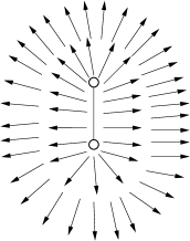
After symmetry breaking, the vortices of non-integer charge are confined. It is conceivable that there are noninteger charges in this phase, connected together by half-line singularities, such that the overall charge is integer. See Figure 4 for an example of a hadronic composite of two charge vortices.
As mentioned, the crucial characteristic of confined excitations is that the condensate takes on a different value to the left and right of the excitation. We started by condensing the order parameter field, such that it took on the value everywhere. Now we have an excitation such that the order parameter field takes the value to the left, and to the right of the half-line singularity connected to the excitation. To unambiguously define the vacuum state , we must make a choice how we treat the excitations. This we do by specifying that excitations, both confined and unconfined, enter the system from the left. Thus, we set , and as a confined excitation comes in from the left the condensate to the left of the excitation takes on the value . If an unconfined excitation comes in from the left, then .
Imagine a particle in a state coming in from the left. We want to know whether is confined of not, i.e. we need to know if , in which case is unconfined. This is where braiding comes in: is the outcome of half-braiding counterclockwise around . Thus, to find out whether is confined, we braid the condensate around the excitation, using the braid operator . For to be unconfined, the condensate has to braid trivially around , both clockwise and counterclockwise. We must check that both braidings are trivial, because the half-line singularity could run along the positive or the negative x-axis in fig. 4. This leads to the following test of whether an excitation is confined or unconfined:
| is unconfined | ||
Let us apply this criterion to the vortices in the XY model, to see which ones are unconfined. Denote a vortex of charge by . We set . Then gets frame dragged as we braid it counterclockwise around , and picks up a phase factor . Clockwise braiding is trivial, since we’ve chosen the convention that the clockwise braiding of an electric mode to the right of a defect is trivial7. Thus
and a vortex is unconfined . Thus the defects are precisely the unconfined vortices.
In the high temperature phase, the “electric” excitations are irreps of the electric group . If we also consider projective irreps, then the electric excitations are irreps of the universal covering group of . The irreps are denoted by , they are labelled by an . All these irreps braid trivially with the condensate , because the condensate is in a state in an electric irrep, and electric irreps braid trivially with each other. Thus in the ordered phase all the electric excitations are unconfined. The situation is different from the situation where defects condense as is discussed in [4].
So indeed the phase transition from the high temperature to the ordered phase in the XY-model can in this sense be described as a confining transition.
3 Hopf symmetry breaking: the formalism
In this section we will first study symmetry breaking for a phase described by a general Hopf algebra . Then we will specialize to the cases where is a modified quantum double: . The quantum double is a special case of the modified quantum double, with .
3.1 The criterion for symmetry breaking
We consider a physical system whose excitations (or particles) are labeled by irreps of a quasitriangular Hopf algebra . We say that a condensate forms in a state of an irrep of , so that our ground state is a state filled with the particles in the state . We now have to define the residual symmetry algebra , which is a symmetry algebra with the property that the excitations of the new ground state form irreps of .
The residual symmetry algebra consists of the operators that are ‘well defined with respect to the condensate’. Before we explain what that means, let us first consider the case of a system whose symmetry is an ordinary group . is broken spontaneously to by a condensate in a state of an irrep of . is the stabilizer of , i.e. the subset of symmetry transformations in that leave the condensate invariant. And because they leave the condensate invariant we can implement these transformations on excitations of the condensate. Thus they act on the excitations, and since by definition they also commute with the Hamiltonian, they transform low energy excitations into excitations of same energy, which can therefore be organized in irreps of H .
Now consider a particle in state of an irrep of the original symmetry . If we fuse with , and act on the outcome of this fusion with an , the result is the same as when we act on with first, and then fuse the outcome with . This follows from
| (15) |
since . Thus we can also define the residual symmetry group to be the set of transformations that are insensitive to fusion with the condensate. Whether a particle in an irrep of fuses with the condensate or not, the action of is the same. Thus we define residual symmetry operators to be operators that are not affected by fusion with the condensate. When the symmetry is spontaneously broken from to , the residual symmetry operators are the elements of .
This definition of residual symmetry operator can be carried over to the case of a condensate in an irrep of a Hopf symmetry . The residual symmetry operators are the operators that are not affected by fusion with the condensate. The residual symmetry operators form a subalgebra of , which we call the residual symmetry algebra . There is a subtlety in the definition of : an operator is an element of if its action on any particle in any irrep of is the same whether has fused with the condensate or not. But we must specify whether fuses with from the left or the right! Namely, in the systems we are considering and are not (necessarily) the same state, because of the possibility of nontrivial braiding. Thus we have to fix a convention. This convention is set by our earlier choice of having all particles come in from the left. Remember that we had to make this choice because some excitations of the condensate may be confined. Thus we define as follows: for any particle in any irrep of , we have
| (16) |
Since and are states of particles of , their fusion is set by the coproduct of :
| (17) |
where is in the irrep of , and in the irrep of . Since this equation has to hold for all vectors in all irreps of , it is equivalent to8
| (18) |
consists of all operators that satisfy this criterion. We will now prove that is a subalgebra of . We also prove two more properties of which will play a role later on.
Lemma 1
The elements of a finite dimensional Hopf algebra that satisfy
form a subalgebra of that satisfies:
-
1.
-
2.
The elements of leave tensor products of the vacuum invariant.
[Proof.]
That is an algebra follows from the fact that is an algebra morphism.
-
1.
Using the definition of and the coassociativity of the coproduct,
-
2.
We just proved that . Using this, we get
We call the right residual symmetry algebra.
What if we condense the sum of two vectors in different irreps,
? According to (18),
is part of the right residual symmetry algebra of
if
| (19) | |||||
Since we are dealing with irreps, the only way to get an equality is
by equating the first terms on the left-hand side and right-hand
side of this equation, and the last terms, separately. So , the intersection of the right residual
symmetry algebras of and . Therefore, we need
only treat the condensation of vectors in one irrep, since we can
then take intersections of the right residual symmetry algebras of
condensates in different irreps to get the right residual symmetry
algebra for
any condensate.
We will now specialize to the case where is a modified quantum double:
where and are groups (see Appendix A).
The irreps of are labelled by an orbit in under the action of , and an irrep of the normalizer of a preferred element .
In Appendix A we show how to write elements of as functions . In this notation the derivations to come are more elegant. Consider symmetry breaking by a condensate in an irrep of .
Lemma 2
Take . Then
| (20) | |||||
[Proof.] We use the formulae in Appendix A.
was obtained by condensing to the right of our system. If we choose to condense to the left, we get another residual symmetry algebra:
| (21) |
We call the left residual symmetry algebra.
It is interesting to compare this criterion to the one in [2]. There, the residual symmetry algebra is denoted by , and is defined as the largest Hopf subalgebra of whose elements satisfy
| (22) |
The motivation for this criterion is: The residual symmetry operators act on the condensate like the vacuum irrep does.
The important difference between and is that we don’t require to be a Hopf algebra. In particular, we don’t expect the residual symmetry to have a coproduct. In fact there is a physical reason why we don’t need to have a coproduct for . We have chosen the condensate to be on the right. If we bring in a confined excitation from the left, the condensate will be in a state to the left of this excitation. Now consider a second particle coming in from the left, it sees the condensate , and it is therefore an excitation associated with the residual symmetry of , which needn’t be equal to the residual symmetry of ! Thus, we have to keep track of the ordering of the particles, i.e. it is crucial to know in which order we brought in the particles from the left. We will see that - not surprisingly - this translates into the absence of a coproduct in , namely we can’t simply fuse irreps of . Before we can discuss this in more detail, we need to take a closer look at the structure of the residual symmetry algebras.
3.2 Relationship between , and
We will now establish a number of interesting connections between , and . All the operators in and satisfy (22):
Thus the operators of and act on the condensate like the vacuum irrep does, just as the operators of do. At the same time, we have the inclusions
| (23) |
The left and right residual symmetry algebras contains . We prove these statements in the following lemma.
Lemma 3
and satisfy the following:
-
1.
All elements of and of satisfy (22):
-
2.
[Proof.]
-
1.
implies:
where we used one the axioms of a Hopf algebra: . This proves the claim for . The proof for is analogous.
-
2.
is a Hopf algebra, so
This proves . The proof that is analogous.
and are not necessarily Hopf algebras, while is a Hopf algebra by definition. It turns out that is a Hopf algebra ! Similarly, is a Hopf algebra . Also, . Thus and are interesting extensions of : if they are equal to each other, then they are equal to . Thus, the difference between and is a measure of the departure of (and ) from being a Hopf algebra.
We need one assumption about to prove these propositions: the antipode of must satisfy . Modified quantum doubles, for example, satisfy this property.
First we prove a little lemma.
Lemma 4
If the antipode of satisfies , then and .
[Proof.] According to (86), and using :
Say , then using the last equation
| Apply to left the and right, and use and to get | ||
So . Similarly we can prove that . Since is invertible, we have and , where is the dimension as a vector space. Therefore, using and , we get
| (24) |
Thus . Since , we must have . Applying to both side of this equation, we get . This lemma states that the antipode brings us from to , and back. In appendix A we show how is used to construct the antiparticle or conjugate irrep of a given irrep. Thus, going from to is tantamount to replacing all particles by their antiparticles!
Using lemma 4, we can prove all our propositions about the relationships between , and .
Proposition 5
For an n-dimensional Hopf algebra whose antipode satisfies , we have
[Proof.]
-
•
We assume . Take . To prove that is a Hopf subalgebra of , we need to prove three things:(25) The first demand is trivial, because , so that
(26) For the second demand: since , we have , and . Choose a basis of , and a basis of . Then
Write out in terms of the bases of and of : Now for . Using lemma 4, .
Thus is a Hopf subalgebra of .
-
•
According to lemma 3, we have , and all satisfy . was defined as the largest Hopf subalgebra of whose elements satisfy , so if is a Hopf algebra we must have . -
•
We already proved that . Thus if we assume we have .Since , is a Hopf algebra. Thus . From lemma 4, we know that . Thus .
Done: .
-
•
Obvious. -
•
Lemma 4 taught us that and . Apply to the left and right of to obtain . Done: .
3.3 and : Hopf or not?
We are interested in finding out which condensates yield a right residual symmetry algebra that is a Hopf algebra. From proposition 5 we know that is a Hopf algebra is the same Hopf algebra.
As a rather general case, consider a phase with a modified quantum double as its Hopf symmetry: . We can write elements of as functions (see appendix A). Now condense in an irrep of . We saw in lemma 2 that a function is an element of if it satisfies
where is the preferred element of .
Analogously to the derivation of lemma 2, we can prove that the functions in are precisely those that satisfy
| (27) | |||||
Proposition 5(4) tells us that proving that is a Hopf algebra is equivalent to proving that . Thus, to prove that is a Hopf algebra, we must prove that if a function satisfies (27), it automatically satisfies (20):
| (28) |
This implication is automatically satisfied if is an abelian group, because then and commute. Thus, if the magnetic group is abelian, is necessarily a Hopf algebra.
Also, if is in the center of , and is acted on trivially by all of , then (28) is satisfied. Electric condensates are an example, since for electric condensates. is in the center of , and acts trivially on .
If the original phase is a phase, then we have similar results: is a Hopf algebra if is abelian, or if is in the center of . We needn’t demand that all of acts trivially on , since this immediately follows from being in the center of .
3.4 Requirement on the condensate
If the condensate is , then our ground state is filled with the particles in the state . We know that if an excitation of this ground state braids nontrivially with the condensate, then it is connected to a domain wall which costs a finite amount of energy per unit length. Thus, if were to braid nontrivially with itself, it wouldn’t make sense to think of a condensate. Thus we require of our condensate that it braid trivially with itself:
| (29) |
Note that we are braiding indistinguishable particles, and if has spin , then the braiding picks up an extra phase factor . The spin factor should be taken into account when verifying the trivial self braiding condition.
Recently fermionic condensates have received considerable theoretical and experimental attention[28], and we could definitely treat those as well with our methods. We may then relax the trivial self braiding condition exactly because identical fermions don’t braid trivially with each other: they pick up a minus sign under half-braiding.
3.5 Unconfined excitations and the algebra
3.5.1 The conditions of trivial braiding
Now that we’ve learned how to derive , we want to study the unconfined excitations of . We found a criterion for determining whether an excitation was confined: If the excitation doesn’t braid trivially with the condensate , then it is confined.
The condensate is in a state of an irrep of . Now consider an excitation of the ground state, sitting in an irrep of . Since the universal R matrix , we cannot simply act with on states in the tensor product representation , because we can only act with elements of on states of . We need a projection of onto , so that we can act with on states of . If has an inner product, then we can use this inner product to define the projection P. Take an orthonormal basis of , and an orthonormal basis9 of . Together, the and form an orthonormal basis of , such that the span , and for all and we have 10
| (30) |
where denotes the inner product between and . Now take any , and write
| (31) |
Thus we have our projection: . It is known that this projection is in fact independent of our choice of basis: given a vector space with an inner product, the perpendicular projection onto a vector subspace is uniquely defined.
Modified quantum doubles come equipped with an inner product (107):
We use this inner product to define the projection operator , just as we discussed above. Now we can define the braiding of a state of with :
| Counterclockwise | (32) | ||||
| Clockwise | (33) |
where in the second line we used: .
We want to find out which irreps of braid trivially with the condensate, thus the braiding has to be trivial for all in the vector space on which acts. We still need a definition of ”trivial braiding”. A natural definition is: braids trivially with the condensate if it braids just like the vacuum irrep does. This definition immediately implies that the vacuum irrep is unconfined, since obviously braids like does. Thus the conditions for trivial braiding of an irrep of with the condensate living in the irrep of become
| (34) |
| (35) | |||||
is an unit matrix, where is the dimensionality of the irrep .
If these equations are satisfied, then we can replace in these equations by for any state of . Thus if satisfies the trivial braiding conditions (34) and (35), then all the states of braid trivially with .
An irrep that satisfies these two equations is said to braid trivially with the condensate. If an irrep doesn’t braid trivially with the condensate, it is a confined excitation, attached to a physical string that goes out to infinity which costs a finite amount of energy per unit length.
3.5.2 The unconfined symmetry algebra
The trivial braiding equations (34) and (35) divide the irreps of into confined and unconfined irreps. We cannot simply take the tensor product of irreps of , since isn’t a Hopf algebra. The reason for the absence of a coproduct is the presence of confined excitations. The condensate to the right of a confined excitation takes on the value , while it takes on a different value to the left of the excitation. Thus particles coming in from the left see a different condensate: they are excitations of the residual symmetry algebra of .
The situation is actually a little more complicated, because the value of the condensate to the left of a state of an irrep of depends on the explicit state of . Thus is not unique for an irrep .
We will discuss how to deal with these issues later. For now, we note that unconfined excitations do not suffer from such complications, since the condensate takes on a constant value around unconfined excitations. Thus we expect the fusion rules of unconfined excitations to be associative, if we only consider their composition with other unconfined excitations. There should be a Hopf algebra , called the unconfined symmetry algebra, whose irreps are precisely the unconfined irreps, and whose fusion rules give the fusion channels of the unconfined excitations into other unconfined excitations.
To obtain , we first determine all unconfined irreps of . Then we take the intersection of the kernels of all unconfined irreps11, and denote it by . Finally, we define the algebra
| (36) |
This is an algebra because is an ideal (i.e. an invariant subalgebra) of . Its irreps are precisely the unconfined irreps.
Our claim is that is a Hopf algebra. Though we have not attempted to prove this in full generality, we found it to be true in all the cases we’ve worked out. In view of our discussion earlier, it is physically natural that is a Hopf algebra, while needn’t be. However the mathematical proof if this conjecture may not be so easy, and this definitely deserves further study. Such a proof should make use of the trivial self braiding condition (29) that we formulated for the condensate , because if this condition is dropped then we have found cases where isn’t a Hopf algebra.
3.5.3 Trivial braiding for
In the next section, we will see that for the electric and defect condensates in a phase with symmetry, the residual symmetry algebra takes on a special form:
| (37) |
where is a subgroup of , and is a subgroup of whose elements satisfy
| (38) |
This last equation tells us that the action of on is well defined: is a modified quantum double, so that the action of on satisfies (108):
Since , all also satisfy this equation. The action of on is given by:
| (39) |
is a transformation group algebra, so we can use the canonical theorem on the irreps of transformation group algebras given in Appendix A. The irreps are labelled by an orbit in under the action of , and an irrep of the normalizer of a preferred element of . We denote irreps of by . The conditions (34) and (35) for to braid trivially with in reduce to
| (40) |
| (41) | |||||
where the and are chosen representatives of left cosets of .
The proof of these equations is rather lengthy. Some intermediate steps are
When the modified quantum double is a quantum double , the conditions for an irrep of to braid trivially with the condensate become
| (42) |
| (43) | |||||
We will now use these equations to work out and for various condensates in modified quantum doubles. We start with electric condensates, and show that the conventional theory of electric condensates (Landau’s theory) is reproduced. After that we study a variety of defect condensates.
4 Condensates in modified quantum doubles
In the previous sections we formulated the general conditions which determine the residual symmetries in the case where a Hopf symmetry is spontaneously broken by the formation of a condensate in a state . We were led to consider an intermediate algebra (or ) and an unconfined algebra which would be manifest in the low energy spectrum of the broken phase. In this section we will present some rather general derivations of and for certain classes of vacua .
We start with a brief discussion of ”conventional” symmetry breaking by an ordinary (electric) type condensate. We recover the well known results with the added feature that the confinement of certain types of defect follows from our formalism. This was already obtained in [2], but with a different definition of the residual symmetry algebra.
In the next subsection we analyze the situations that arise if one considers defect condensates. We point out that these can be of various types leading to different low energy phenomena. We refrain from discussing the case of mixed (or dyonic) condensates. These can definitely be studied using our formalism, but they have to be dealt with on a case to case basis, while for the case of ordinary and defect condensates we were able to extract general formulae.
4.1 Ordinary (electric) condensates
Consider a phase described by a quantum double , and condense a state of an electric irrep of . Then equation (20) tells us that the functions in satisfy
where is the stabilizer of , i.e. the set of elements that satisfy . 1 is the unit matrix. Since the condensate is purely electric, the magnetic group is unbroken, thus all of is present in . is a Hopf algebra in this case, which implies that the tensor product of irreps is well defined, and associative.
Some defects are confined. The trivial braiding conditions (42) and (43) tell us that only the defects are unconfined. Thus the unconfined symmetry algebra is
| (45) |
One of the consequences of electric symmetry breaking is the lifting of degeneracies. Namely, excitations which used to be in the same irrep are now split into different irreps, which may have different energies. This splitting of energy levels is experimentally measurable, in principle.
To treat a phase with inversion symmetry, such as an achiral tetrahedral nematic with symmetry (see [3]), we need the formulae for electric symmetry breaking of modified quantum doubles . The derivation of and after the condensation of a state of an electric irrep of a modified quantum double is analogous to the derivation given above for a quantum double . The result is
| (46) | |||
| (47) |
For example, for , , so that .
As an example, we’ve worked out all possible electric breaking patters from , see table 1. Although we haven’t found references that systematically work out all electric condensates for all irreps as we have done, the theory behind electric condensates is well known and in that sense this is nothing new. Our interest was to rederive the results for ordinary condensates from the Hopf symmetry description of liquid crystals. A reference that offers a detailed analysis of the theory of ordinary condensates in bent-core nematic liquid crystals is [29], where a wealth of non-abelian phases are discussed. An analysis of the order of the phase transitions using Renormalization group calculations is done in [30].
| Original symmetry | Irrep | ||
|---|---|---|---|
| of condensate | |||
As a side note, the transition from to in table 1, induced by the condensate of a state in the irrep of , is an example of spontaneous symmetry breaking from an achiral to a chiral phase, since does not contain any inversions or reflections, while does. This may be the explanation of the experimental discovery of a phase built up of achiral molecules, whose symmetry is spontaneously broken to a chiral phase[32]. For a relevant discussion, see [29].
4.2 Defect (magnetic) condensates
There are different types of defect condensates which we wish to analyze. Consider a phase described by a quantum double , or a modified quantum double , and pick a magnetic representation ( is the trivial representation of the centralizer ). A basis of the vector space on which this irrep acts is given by , where the are the different defects in . We consider the following types of condensates:
-
•
Single defect condensate
(48) -
•
Class sum defect condensate
(49) where is a conjugacy class in the case, and an orbit in under the action of in the case. We denote the condensate by , where is the preferred element of .
-
•
Combined defect condensate
(50) where is a subset of the defects in one class. We need only take the elements to be within one class because, as we mentioned earlier, we need only study the cases where the condensate is the sum of vectors in the same irrep.
The single defect and class sum defect condensates are a special case of combined defect condensate. The derivation of and for a combined defect condensate is rather technical, so we will discuss the results for the single defect and class sum defect condensates first, and then derive the general formulae.
4.2.1 Single defect condensate
Consider a phase with symmetry, and condense in the magnetic irrep . We’re condensing the chosen preferred element in the conjugacy class . This is not a restriction on our choice of defect, since was chosen arbitrarily. The condensate satisfies the trivial self braiding condition (29).
The function that corresponds to the vector is (see appendix A)
| (51) |
The criterion (20) that defines becomes
| (52) |
where we define to be the smallest subgroup of that contains .
This result for has a very natural interpretation: the residual electric group is , the subgroup of that doesn’t conjugate the defect. The magnetic part is not necessarily a group. It consists of left cosets of . The defects are now defined modulo the condensate defect . In other words, if a particle in a magnetic irrep of the residual symmetry fuses with the condensate , it is left unchanged. Thus its defect is defined modulo .
Using our previous propositions, we can prove that is a Hopf algebra is a normal subgroup of is a group.
The unconfined symmetry algebra is
| (53) |
If we condense another defect in the conjugacy class , the symmetry algebras are12 :
| (54) | |||
| (55) |
The results for a single defect condensate in a phase with symmetry are analogous:
| (56) | |||
| (57) |
As an example, we’ve worked out all single defect condensates in an achiral tetrahedral nematic in table 2. For a discussion of the derivation of these results, and for single defect condensates in octahedral and icosahedral nematics, see [3].
| Single defect condensate in | |||
|---|---|---|---|
4.2.2 Class sum defect condensates
Consider a phase with symmetry, and condense the sum of the defects in the conjugacy class :
A class sum defect condensate satisfies the trivial self braiding condition (29):
In going from the second to the third line, we use the fact that for any .
A class sum condensate doesn’t break the electric group at all! Namely, conjugation acts trivially on a conjugacy class, since for any we have
| (58) |
Thus this condensate is invariant under all residual symmetry transformations in . For this reason, in the case of a local gauge theory this condensate is indeed the only physically admissible gauge invariant magnetic condensate. Namely, in the phase of a gauge theory, with a discrete group, the only residual gauge transformations are global, because is discrete and the gauge transformation must be continuously defined on the space. These gauge transformations act trivially on the class sum defect condensates, thus these condensates are indeed gauge invariant.
The residual and unconfined symmetry algebras are
| (59) | |||
| (60) |
where is the smallest subgroup of that contains the class . From this definition, it follows that is a normal subgroup of . Thus is a group.
If we condense a class sum defect condensate in a modified quantum double , the outcome is
| (61) | |||
| (62) |
As an example, we’ve derived all class sum defect condensates in an achiral tetrahedral nematic in table 3. The class sum defect condensates in an achiral octahedral, and an achiral icosahedral nematic are discussed in [3].
| Defect conjugacy classes of | |||
|---|---|---|---|
4.2.3 Combined defect condensates
The formal derivation
We will now derive all the formulae for defect condensates we have come across.
Start with a phase with symmetry. Choose an irrep , and consider a condensate of the form , with a subset of the defects in one conjugacy class.
The demand of trivial self braiding (29) gives
| (63) | |||||
It would be interesting in itself to construct the general solution to this constraint, and to determine how many different defect condensates satisfy this criterion. For example the defect-antidefect condensate always satisfies this criterion13, as does the superposition any set of commuting elements in a certain conjugacy class, and class sum defect condensates. This trivial self braiding condition will play a crucial role in determining .
The derivation of and is rather formal. We give the results first, and then we derive them:
For the derivation, we must introduce various definitions. Define the following subset of (which needn’t be a subgroup):
| (64) |
where is the normalizer of the chosen preferred element in , and satisfies . In function notation, the condensate wave function is
| (65) |
Define the following subgroup of :
| (66) | |||||
| (67) |
is composed of the global symmetry transformations that leave the condensate invariant.
Also define
| (68) |
Using (121): , we can prove that
| (69) |
From this equation we can derive that the elements of satisfy
| (70) |
Finally, we need one more definition:
| (71) |
where is the smallest subgroup of that all the , i.e. the defects in the condensate.
The trivial self braiding equation (63) implies that . Thus, according to (69) and (70)
| (72) |
The residual symmetry algebra is given by the set of functions that satisfy (20):
| (73) |
We will now prove that
| (74) |
Note that need not be a group.
To prove (74), take . Then such that . Namely, if such an doesn’t exist, then , thus according to (67), and .
Now substitute into (73): so the equation implies for all . Acting with all the on gives us all the , thus for all . Thus, in the first component must be constant on left K cosets, since is generated by the . Thus .
is a little harder to extract. It is given by
| (75) |
For the case of a quantum double
| (76) |
To prove (75) and (76), we must find out which irreps of braid trivially with the condensate in the irrep of .
Our residual symmetry algebra is of the form (37), with and . Thus we can use the conditions (40) and (41) to determine the irreps of that braid trivially with the condensate. The unconfined symmetry algebra is then the Hopf algebra whose irreps are precisely the unconfined irreps.
Equation (40) states that for an unconfined irrep , with the preferred element in the orbit :
| (77) |
where the are chosen representatives of left cosets in .
Using (72), equation (77) becomes
Choosing , we get . (40) is actually equivalent to in this case, because follows from . To prove this, note that , so . Thus
In proving the third equal sign we used the fact that .
Thus (40) has taught us that for an irrep to be unconfined, we must have . The magnetic part of the unconfined symmetry algebra is therefore . From the definition of and , we can prove that
| (78) |
Thus is a normal subgroup of . is the unconfined magnetic group.
Equation (41) further restricts :
Choose an such that . This is equivalent to saying that for some . Now choose in (41):
Now . Since and , we have , so . Thus . Now acts trivially on the magnetic group , due to (121). Thus necessarily , since the elements of are normalizers of all elements of , so they are also normalizers of . This means that . 4.2.3) becomes
Observe that the set . Since must send all to the unit matrix 1, must send all of to the unit matrix (since is generated by ). We conclude that is in the kernel of , and the electric group is .
At the start of this last derivation, we filled in in (41). The case gives nothing new, because
| (79) |
where in the last line we used a fact that we proved earlier: . Thus (41) becomes
This is equation is satisfied if , which we already proved.
Summarizing, the unconfined magnetic group is , and the unconfined electric irreps are those that have in their kernel, which means that the electric group is . Thus we have derived (75). Had we started with a quantum double (), the unconfined symmetry algebra becomes , because in that case .
Acknowledgement: F.A.B. would like to thank the Yukawa Institute for Theoretical Physics in Kyoto, and in particular prof. R. Sasaki for their hospitality. Part of the work was done while visiting there.
Appendix A Quasitriangular Hopf algebras
In this appendix we summarize the mathematical structure and notation connected to the Hopf algebras, which are extensively used in this paper and in previous literature. The applications focus on the quantum double of a finite (possibly non-abelian) group . The essential information is collected in a few comprehensive tables. In the text we merely comment on the meaning and the physical interpretation/relevance of the basic concepts. We conclude with a discussion of modified quantum doubles.
Algebras are an ubiquitous mathematical structure. Another - maybe less familiar mathematical notion - is that of a coalgebra, a structure that is in a precise sense a dual object to an algebra. A Hopf algebra is simultaneously an algebra and a coalgebra, with certain compatibility conditions between the two structures. In the following subsections we systematically go through some definitions and important examples.
A.1 Algebras, coalgebras, and their duals
An algebra is a vector space over a field (which we will take to be ), with a bilinear multiplication. We can think of the multiplication as a map . The algebras we discuss will all have a unit element, i.e. an element which satisfies . Thinking of it as a map one could say that the unit embeds the field into the center of the algebra. We write . We require that be an algebra morphism (the field is also an algebra, with itself as ground field). The algebras we consider are associative with respect to their multiplication.
An important example for our purposes is the group algebra
of a finite group. Label the groups elements by . The group
algebra is then the set of objects of the form , with . This algebra is important,
as it contains all the information about the group. For example,
irreducible representations of the group algebra are in one-to-one
correspondence with irreducible representations of the group.
In the physical models we consider, the regular (electric) modes
transform under an irrep of the group, which is equivalent to
saying that they transform under an irrep of the corresponding
group algebra.
A coalgebra is a vector space equipped with a comultiplication and counit. The comultiplication is a linear map . The counit is a linear map . They must satisfy the formal relations:
We see in Table 4 that the group algebra naturally has a coalgebra structure, where the comultiplication defines the action of the group on the tensor product space.
Given an algebra , its dual14 can be given a natural coalgebra structure. Similarly, given a finite dimensional coalgebra, its dual has a algebra structure (in a slightly less natural way reminiscent of the isomorphism for a finite dimensional vector space). The structure of the duals are given in Table 4, and the structures are given explicitly for the group algebra and the function algebra, which are each other’s duals. An example of a dual structure is the following: given a coalgebra with a coproduct , the dual has the following multiplication (which we denote by a star ): . Thus the coproduct of is used to define the multiplication in . Similarly, the counit of is used to define the unit in .
| Hopf algebra | Dual Hopf algebra | |||
| e.g.: Group algebra | Functions on the group | |||
| Basis: {} | ||||
| Algebra | Dual algebra | |||
| product | ||||
| unit | ||||
| Co-algebra | Dual co-algebra | |||
| co-product | ||||
| co-unit | ||||
| antipode | ||||
, the set of functions from to , is the coalgebra dual to the algebra . It is also an algebra, and in fact it is a Hopf algebra (see next section). These functions form a vector space, which is spanned by the functions15 with . A coalgebra structure is then defined by
| (80) |
We need only define these functions on a basis of since they are linear.
Using the definition of the coproduct one arrives upon evaluation
on a pair of elements of at,
| (81) |
A.2 Hopf algebra’s
A Hopf algebra is simultaneously an algebra and a coalgebra, with
certain compatibility conditions. Namely, we demand that
and be algebra morphisms. This is equivalent
to demanding that and
be coalgebra morphisms (see [33]).
A Hopf algebra also contains an antipodal map , which is the
unique map from to that satisfies
| (82) |
From this definition, one can derive the following relations:
| (86) | |||||
Physically, the antipode map is used to construct antiparticle representations out of particle representations. This will become clear if we are to talk about representation theory, where given an irrep , we define the antiparticle or conjugate irrep as , where denotes transposition. is an irrep because is an antimorphism, and so is the transposition. When we fuse particle and antiparticle irreps, we don’t necessarily get the vacuum representation, but it is guaranteed that is present in the fusion rules. This is completely analogous to the case of ordinary groups.
The standard example of a Hopf algebra is the group algebra. We have already discussed the algebraic and coalgebraic structure. It is turned into a Hopf algebra by defining the antipode as the inverse:
| (87) |
So in fact all the familiar ingredients of a group(algebra) make it already into a Hopf algebra. Given a finite dimensional Hopf algebra , one can quite generally define a Hopf algebra structure on , and is then called the dual Hopf algebra. The definitions are quite natural and are given in Table 4. Note that for the dual Hopf algebra the antipodal map again involves the inverse, in the sense that .
In the context of our physical applications, the dual version of the algebra has very much to do with the topological defects and could be called the “magnetic” part of the algebra. When we have discussed the representation theory it will become clear what the physical states are and what the action of the elements of the dual algebra mean. One thing that may already be clear at this point is that, if the topological charge corresponds to a group element, then the comultiplication of the dual or function algebra determines the action on the tensor product representation of the dual, and therefore describes the fusion properties of the defects. It is then clear from the expressions (A.1) and (A.1) that the fusion indeed leads to the required multiplication of group elements.
A.3 Quasitriangularity
A Hopf algebra is called quasitriangular when there is an invertible element of that satisfies:
| (88) | |||||
| (89) |
where if we write , then
where is in the i-th, and in the j-th position.
The action of the R element on a tensorproduct of two representations is to “braid” the two particles and is of crucial importance to get the complete physical picture of particles and defects which exhibit nontrivial braid properties. From the first equations (88) one derives that the Yang-Baxter equation is satisfied. Equation (89) is the important statement that the generators of the braid group commute with the action of the Hopf algebra. This leads to the decomposition of multi-particle states in product representations of the braid and the Hopf algebra, thereby allowing for a clear definition of what we mean by quantum statistics and nonabelian anyons, etc. We will return to this subject shortly.
A.4 The quantum double
| Double algebra | ||
| Ex: Hopf double algebra | ||
| Basis: {} | ||
| Algebra | ||
| product | ||
| unit | ||
| Co-algebra | ||
| co-product | ||
| co-unit | ||
| antipode | ||
| Central (ribbon) element | ||
| R-element | ||
Given a Hopf algebra , there is a natural way to “double”
it, creating a new Hopf algebra called Drinfeld’s quantum
double of . As a vector space, , so it’s a tensor product of and its dual. For the
discussion of the Hopf algebra structure on , see
[33]. For our purposes, we need only know what the
structure is like for a discrete group. We also
specify a braid matrix, making it a quasitriangular Hopf algebra.
As vector space, is , which is the same as
for finite . Denote the basis elements of
as or (the latter is the notation used in
[6]), where , and is defined by
().
If we look upon as an
element of , the function it corresponds to is . We can also define , and . We’ve therefore
embedded and into , and from these embeddings
obtained a basis of (meaning that any element can be written
as a sum of products of these basis elements). The structure of
is set by the following formulae:
| (90) | |||
| (91) | |||
| (92) | |||
| (93) | |||
| (94) |
The complete structure is summarized in Table 5, including the ribbon element (discussed later).
These relations can also be given in the language of functions in . The notation that comes along with this formulation proves very convenient in actual calculations, so it is useful to give the corresponding definitions here:
| (95) | |||
| (96) | |||
| (97) | |||
| (98) | |||
| (99) |
This formulation is also important because it can be carried over to define the quantum doubles of continuous groups , where is compact, or locally compact. For results on such cases, see [34] and [35].
We finally should mention that the quantum double has a central element, denoted by and called the ribbon element. Its eigenvalue can be used as a label on the representations of the . In applications it defines the phase obtained after rotating the particle state by and is therefore called the spin factor of a given representation. It plays a central role in defining a suitable generalization of the spin statistics connection, to which we turn next.
A.5 A non-Abelian spin statistics connection
Let us briefly return to the important role played by the element which as mentioned, generates the action of the braid group on a multi-particle states corresponding to some state in a tensor product of representations of . We noted already that the braiding with commutes with action of :
| (100) |
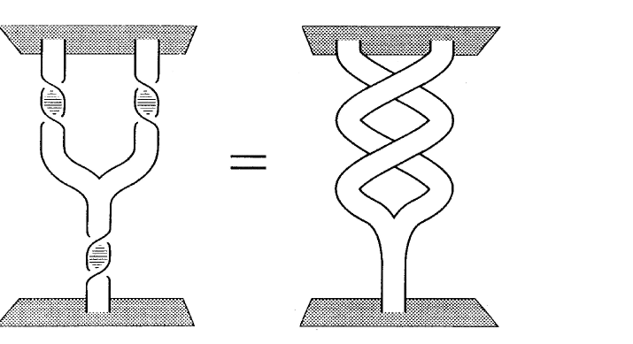
where (i.e. followed by a trivial permutation of the two strands). From this it follows that the -particle states form representations of , with the braid group on strands. We speak of non-abelian statistics if the theory realizes states that correspond to higher dimensional representations of . In this context it is an important question to what extent one can still speak of a spin-statistics connection. One can indeed write down a generalized spin-statistics theorem in terms of the action of the braid group end the central ribbon element which corresponds to physically rotating the defect over an angle and therefore generating the phase factor due to the (fractional) spin of the particle in question. It reads:
| (101) |
and can be represented graphically by the “suspenders diagram” depicted in Figure 6. Note that the concept of a spin statistics connection has become considerably more intricate. It is no longer an attribute carried by a single particle. It may involve two different particles (mutual statistics) and is also dependent on the channel in which they are fused.
A.6 Representation theory
The irreducible representations of follow from the observation that it’s a transformation group algebra (see [2] for details). Since we will come across other transformation group algebras in the main text, we give the general definition. As a vector space, the transformation group algebra is , where is a finite set and is a finite group. A basis is given by
| (102) |
Just as in the quantum double case, we can consider it to be the vector space of functions
| (103) |
The element corresponds to the function
| (104) |
Furthermore, there is an action of the group on . This means that the elements act as bijections of , in a manner that is consistent with the group structure (i.e. we have a homomorphism from to bijections of ). Denote the action of on by . We now turn this vector into an algebra, by introducing a multiplication.
Definition 6
is a transformation group algebra if the multiplication of and is given by:
| (105) |
In function notation:
| (106) |
We define an inner product on . We give it in both notations: in terms of elements , and in terms of functions .
| (107) |
We can split up into orbits under the action of . The orbit of an is given by . Call the collection of orbits. For each orbit , choose a preferred element , and define the normalizer to be the subgroup of that satisfy . The and play a central role in the determination of the irreps.
Theorem 7
Choose an orbit in , a preferred element of ,
and an irrep of . The orbit
. Let be any
element in such that . Then the
form representatives of left cosets in . Further
call the basis vectors
of the vector space on which the irrep acts.
An irreducible unitary representation of
is given by inducing the irrep . A basis of
the vector space is , and the action of
is given by
where is defined by . This is
possible because sits in a particular
coset of , and the are representatives of the left cosets.
Furthermore, all unitary irreducible representations are
equivalent to some , and is
equivalent to iff and is
equivalent to .
Thus irreps of a transformation group algebra are labelled by an orbit in under the action of , and an irrep of the normalizer of a chosen preferred element of .
The notation in terms of basis elements makes the action of the irreps transparent. An alternate notation for the Hilbert space is . Then the action of a global symmetry transformation is simply
In words, the part of g that ”shoots through” the defect acts on the electric part.
| Representations of | ||
|---|---|---|
| representation | defect/magnetic label, ordinary/electric label | |
| Conjugacy class (orbit of representative element ). | ||
| is a representation of the normalizer of in . | ||
| carrier space | ||
| action of on | ||
| central element | ||
| spin factor | ||
| tensor products | ||
| Clebsch-Gordan series: | ||
The function notation is rather opaque, but extremely useful in calculations in the main text. The Hilbert space of the irrep is given by:
To make contact with the notation above, corresponds to the vector attached to the “flux” . For example, the function associated with is . To explain the rest of the definition, note that
which explains why .
Then the action of on under the irrep
gives a new function , defined by
One easily checks that this is equivalent to the definition given above.
The quantum double is a special case of a transformation group algebra, with and . Thus in the orbits of under the action of are conjugacy class of . is the centralizer of the preferred element of .
We proved earlier on that the antipode can be used to create an antiparticle irrep from any irrep . In the case of , the antiparticle irrep of is , where is the conjugacy class of , and . In particle, for an electric irrep the antiparticle irrep is . An example of this is the 3 irrep of , which is the antiparticle irrep of 3. The quarks transform under the 3 irrep, while the antiquarks transform under the irrep of .
A.7 Modified quantum doubles
In the main text we came across phases whose Hopf symmetry was a variation on a quantum double, which we called a modified quantum double. We will now give the general definition of a modified quantum double16.
As a vector space a modified quantum double is , where and are two groups. It is also a transformation group algebra, so there is an action of on . We denote the action of on by . We require this action to satisfy the following relation:
| (108) |
A basis of is given by . is a Hopf algebra with the following structure:
| (112) | |||||
These structures satisfy all the axioms of a Hopf algebra, thus is a Hopf algebra. Just as in the quantum double case, we can write elements of as functions in . An element of is a function
| (113) |
The element corresponds to the function
| (114) |
The structures of are
| (115) | |||
| (116) | |||
| (117) | |||
| (118) |
Making quasitriangular, i.e. introducing a braid matrix, is not that easy. We have found a way to do it that applies to all physical systems we looked at. We need a homomorphism:
| (119) |
that satisfies the following relations:
| (120) | |||
| (121) | |||
| (122) |
is then a quasitriangular Hopf algebra with the following braid matrix:
| (123) |
The inverse of is
| (124) |
The quantum double is a special case of a modified quantum double, with , , and .
Appendix B Defining a coproduct for
is not always a Hopf algebra, because the coproduct of does not necessarily satisfy . It does satisfy . This means that we cannot take the tensor product of irreps of , in other words we cannot fuse two particles in . We can only fuse particles in with particles of coming in from the left.
The reason we can’t fuse particles of is that some excitations of the condensate are confined. The condensate takes on the value to the right, and to the left of a confined excitation, in an irrep of . Thus particles coming in from the left see the condensate . Thus particles to the left of are excitations of , and they transform under irreducible representations of the right residual symmetry algebra of .
Matters are complicated further by the observation that given two states and in a confined irrep , the value of the condensate to the left of need not be equal to the value the condensate takes to the left of . Thus the condensate does not take a well defined value to the left of the irrep .
One possible interpretation of a configuration with a confined excitation , is that the condensate has only condensed to the right of . To the left of the system is in the unbroken phase, with symmetry. Thus particles to the left of are irreps of . We can fuse particles in irreps of with , and look at the fusion rules. The outcome of this fusion tells us what the particle in the irrep can become when it enters the ordered phase.
This interpretation of a confined excitation is reasonable, but it is unsatisfactory. Namely, we still want to be a able to fuse the irreps of the residual symmetry algebra. There should be a finite set of quantum numbers in the broken phase, and we should be able to tell which of these quantum numbers can form hadronic composites. We want to be able to talk about the fusion of the quantum numbers in the broken phase without bringing in the quantum numbers of . We know that if is a Hopf algebra, we can fuse irreps of . We will now discuss how to fuse irreps of when is not a Hopf algebra.
B.1 A purely magnetic phase
Let us first study a simple system that only has magnetic degrees of freedom. Its symmetry algebra is , with some finite group. A basis of is given by , where is a projection operator. It measures the flux of a configuration : if the flux of a state is , then . If the flux of isn’t , then .
Now consider a single defect condensate . Then using (56) (with ) we find for the residual symmetry algebra:
| (125) |
where is the subgroup of generated by . Let us assume that is not a normal subgroup of , so that is not a Hopf algebra. A basis of is given by , where consists of a set of representatives of the left cosets in . These projection operators measure defects modulo the condensed defect . This is a consequence of our definition of operators in : the operators in are the operators that do not notice when a particle fuses with the condensate .
If we apply the coproduct on a basis element of , we obtain
| (126) |
This coproduct has a natural interpretation: if a projection operator measures a defect on the right, then the projection operators on the left measure defects modulo . Thus : the condensate on the left is conjugated by . Note that the defect of the particle that measured is only defined modulo g, but this doesn’t affect , since .
We assume that there is a confined excitation in an of , and that . We have a condensate to the left of the confined excitation measured by that is different from the condensate to the right. We can, however, redefine our projection operators to the left of the confined excitation. The projection operators to the left of are defined modulo . A basis of these projection operators is , where consists of a set of representatives of the left cosets in .
To every projection operator , we associate a projection operator in :
| (127) |
Using this definition, we can define a coproduct for :
| (128) |
is a map from to . One can check that is an algebra morphism, i.e.
| (129) |
We can use to fuse two irreps and of :
| (130) |
is not coassociative, i.e.
| (131) |
This implies that the tensor product of three irreps , and of is not associative:
| (132) |
The interpretation of this non coassociativity is as follows: when we take the tensor product , is defined with respect to the condensate to the right of . If a third particle comes in from the left, then it becomes defined with respect to the condensate between and . So we have a natural ordering for the tensor product, namely we must take , which corresponds to having in the system, then bringing in from the left, and then bringing in . is unphysical, because it isn’t clear how the particles were put in the system.
B.2 The general case
In general, if we bring in from the left in that order, the resulting configuration is . We have been forced to introduce an ordering in our fusion. This ordering corresponds to an ordering in the coproduct:
| (133) |
Once we have defined a non coassociative coproduct , we can fuse confined excitations , and study the possible hadronic composites. To define a , we need a linear map with the following properties:
where was a subideal of such that . The last demand is equivalent to demanding that we do not alter at the level of . Then we define
| (134) |
We can be more explicit in the case of a condensate in a phase described by a modified quantum double , when the right residual symmetry algebra is of the form (37) : . We’ve seen that is of this form for electric condensates, and defect condensates. The action of on is well defined, because acts trivially on . For every orbit in under the action of , pick a preferred element . Now define a map such that . In other words, sends every left coset into a chosen element in . We demand that17 for all
| (135) |
Using , we define
| (136) |
It is straightforward but lengthy to verify that is an algebra morphism18. Thus we have a coproduct
| (137) |
B.3 An example:
As an example, we consider a phase described by the quantum double of the double cover of an even dihedral group: . The group has the following structure:
| (138) |
with .
Now condense a single defect19 . The right residual and unconfined symmetry algebras are
| (139) | |||
| (140) |
where .
The irreps of are given in Table 7, and the irreps of , which occurs as a centralizer of two orbits in , are given in Table 8.
We write the basis of the irrep as , where corresponds to the defect (remember that the defects are defined modulo the condensate ). The action of on this basis is set by
We can write this compactly in one equation:
| (141) |
| Preferred | |||
| element | |||
| Orbit | |||
| in | |||
| Normalizer | = | = | = |
| Irrep of | |||
| Irrep of | |||
| Unconfined | |||
| irreps |
| Element of | ||||||||
|---|---|---|---|---|---|---|---|---|
| Irrep | ||||||||
The left cosets in are . To define the coproduct, we must choose for every . If we choose , then the coproduct is coassociative. This can be traced back to the fact that the form a group. Note that in general, it is not possible to choose representatives of the cosets so that they form a group.
Using , we can determine the following fusion rule:
| (142) |
The unconfined irreps are given in Table 8. This fusion rules implies, for example, that and can fuse to , which is unconfined. Thus we have made a hadronic composite.
If we choose , the fusion rules are the same, even though the coproduct is not coassociative. However, in this case the definition of the particles is altered. Namely, if an irrep is present to the right, then in the irrep coming in from the left should be interpreted as . This can be checked by applying the projection operators:
| (143) |
We have therefore discovered that our choice of coproduct alters the meaning of the labels of our irreps, when they are to the right of a confined excitation. The reason for this is the following: we can determine the irreps of , and that gives us a finite set of labels. When we have one particle in an irrep of in the system, its meaning is unambiguous. Now if a confined excitation is present, then we know that the residual symmetry algebra of the condensate to the left of the excitation may be different from the right residual symmetry algebra . However, we still want to use the same labels for particles to the left of the confined excitations, because they are excitations of a symmetry algebra isomorphic to . Thus we are adding information to the labels of irreps of , namely we are defining their meaning when they appear to the left of a confined excitation. They should not be considered as the same particle: for example, should not be interpreted as the fusion of with itself. The correct interpretation is that we have the confined excitation of , and we brought in a particle from the left, which under our choice of coproduct is labelled by .
In summary, for the condensate in , the fusion rules are independent of the choice of coproduct. We do not expect this to be a general result (although in the cases we’ve worked out the fusion rules don’t depend on the choice of coproduct). The physics of the phase, on the other hand, should not depend on our choice of coproduct, since this choice boils down to a definition of our labels. An interesting follow up on this research would be to study the influence of the choice of coproduct on the fusion rules.
Notes
1 : Modified quantum doubles are a slight variation on quantum doubles. Their precise definition is discussed in Appendix A.
2 : We assume here that is simply connected. If it isn’t, we can take the universal covering group of , and then should be
replaced by the lift of in the universal covering group in all formulae.
3 : A comprehensive summary of the algebraic framework of Hopf algebras, focusing on our specific needs is given in Appendix A. For an extensive introduction to the use of Hopf algebras in the present physical context we refer to [6].
4 : See Appendix A, and for an extensive background [18].
5 : Actually, if we are braiding two indistinguishable electric particles, then the braiding may give a phase factor. Under half-braiding the wavefunction of the system picks up a phase factor , where is the spin of the particles.
6 : The difference with standard Riemann geometry is that one doesn’t assume that the metric is torsion free, i.e. the Christoffel symbols are not required to satisfy . In the Cartan formulation the spin connection and the vielbein are considered as independent, while in Riemannian geometry they are linked by the no torsion condition.
7 : In a gauge theory, this amounts to picking a gauge such that the Dirac string points ‘upwards’ in the drawings. In the global case, we orient the defect such that the frame dragging happens in the upper half plane.
8 : We thank dr. Joost Slingerland for discussions on this point. He studied this relation independently.
9 : is the vector space consisting of all vectors in perpendicular to all vectors in .
10 : We can find such a basis of using the Gram-Schmidt orthogonalization procedure.
11 : The kernel of a map is the set of elements which the irrep maps to zero. These elements form an ideal , meaning that if and , then and .
12 : To prove this, use and .
13 : Note that and needn’t be in the same conjugacy class.
14 : The dual of an algebra is defined as , the set of linear functions from to .
15 : Different, strictly equivalent notations are frequently used here: . In particular we have the identities , the last delta being the usual Kronecker delta.
16 : We came up with this structure to deal with phases with inversion or reflection symmetries. It turns out to be a special case of a bicrossproduct of Hopf algebras, see e.g. [18].
17 : It is not at all clear that this can always be achieved, even though it is possible in the simple cases we’ve looked at.
18 : is not an algebra morphism of , it is only an algebra morphism when restricted to .
19 : We take even dihedral groups, because in , condensing yields , which is slightly less interesting, but note that we can still study hadrons! Only the hadron must be in the trivial irrep, since that is the only unconfined irrep.
References
- [1] F.A. Bais, B.J. Schroers, J.K. Slingerland, Broken quantum symmetry and confinement phases in planar physics, Phys. Rev. Lett. 89 (2002) 181601
- [2] F.A. Bais, B.J. Schroers, J.K. Slingerland, Hopf symmetry breaking and confinement in (2+1)-dimensional gauge theory, JHEP 05 (2003) 068
- [3] C.J.M. Mathy, F.A. Bais, Nematic phases and the breaking of double symmetries, arXiv:cond-mat/0602109, 2006.
- [4] F.A. Bais, C.J.M. Mathy, Defect mediated melting and the breaking of quantum double symmetries, arXiv:cond-mat/0602101, 2006.
- [5] F.A. Bais, P. van Driel, M. de Wild Propitius, Quantum symmetries in discrete gauge theories, Phys. Lett. B280 (1992) 63-70
- [6] M. de Wild Propitius, F.A. Bais, Discrete gauge theories, in: G. Semenoff and L. Vinet (Ed.), Particles and Fields, CRM Series in Mathematical Physics, Springer Verlag, New York, 1998, p. 353-439.
- [7] G.W. Moore, N. Read, NonAbelians in the Fractional Quantum Hall Effect, Nucl. Phys. B360 (1991) 362-396
- [8] N. Read, E. Rezayi, Beyond paired Quantum Hall states: parafermions and incompressible states in the first excited Landau Level, Phys. Rev. B59 (1999) 8084.
- [9] C. Nayak, F. Wilczek, Quantum Hall states of high symmetry, Nucl. Phys. B450 (1995) 558-568.
- [10] J.K. Slingerland, F.A. Bais, Quantum groups and nonabelian braiding in Quantum Hall systems, Nucl. Phys. B612 (2001) 229-290.
- [11] P. Fendley, E. Fradkin, Realizing non-Abelian statistics, Phys. Rev. B72 (2005) 024412.
- [12] F.A. Bais, N.M. Muller, Topological field theory and the quantum double of SU(2), Nucl. Phys. B530 (1998) 349-400.
- [13] A.Y. Kitaev, Fault-tolerant quantum computation by anyons, Ann. Phys. 303 (2003) 2-30.
- [14] J. Preskill, Reliable Quantum Computers, Proc. Roy. Soc. Lond. A454 (1998) 385-410.
- [15] M.H. Freedman, A. Kitaev, Z. Wang, Simulation of topological field theories by quantum computers, Commun. Math. Phys. 227 (2002) 587-603.
- [16] E. Dennis, A. Kitaev, A. Landahl, J. Preskill, Topological quantum memory, J. Math. Phys. 43 (2002) 4452-4505.
- [17] F.A. Bais, Flux metamorphosis, Nucl. Phys. B170 (1980) 32-43.
- [18] S. Majid, Foundations of Quantum Group Theory, Cambridge University Press, 1995.
- [19] M. de Wild Propitius, Topological interactions in broken gauge theories, PhD thesis, Universiteit van Amsterdam, 1995.
- [20] H. Kleinert, Gauge Fields in Condensed Matter, Vol. I: Superflow and Vortex Lines, Disorder Fields, Phase Transitions, World Scientific, Singapore, 1989.
- [21] M.O. Katanaev, Geometric theory of defects, PHYS-USP 48(7) (2005) 675-701.
- [22] M.V. Khazan, Analog of the Aharonov-Bohm effect in superfluid He3-A, JETP Lett. 41 (1985) 486.
- [23] C. Furtado, V.B. Bezerra, F. Moraes, Berry’s quantum phase in media with dislocations, Europhys. Lett. 52 (2000), 1.
- [24] P. McGraw, Global analogue of Cheshire charge, Phys. Rev. D50 (1994) 952-961.
- [25] E. Verlinde, A Note on Braid Statistics and the Non-Abelian Aharonov-Bohm Effect, in: S. Dal (Ed.), International Colloquium on Modern Quantum Field Theory, Bombay 1990, World SCientific, Singapore, 1991.
- [26] J. March-Russell, J. Preskill, F. Wilczek, Internal frame dragging and a global analog of the Aharonov-Bohm effect, Phys. Rev. Lett. 68 (1992) 2567-2571.
- [27] F.A. Bais, The topology of monopoles crossing a phase boundary, Phys. Lett. B98 (1981) 437.
- [28] M. Greiner, C.A. Regal, D.S. Jin, Fermionic condensates, in: AIP Conf. Proc., vol. 77-, 2005, p. 209-217.
- [29] T.C. Lubensky, L. Radzihovsky, Theory of bent-core liquid-crystal phases and phase transitions, Phys. Rev. E 66 (2002) 031704.
- [30] L. Radzihovsky, T.C. Lubensky, Fluctuation-driven 1st-order isotropic-to-tetrahedratic phase transition, Europhys. Lett. 54(2) (2001) 206-212.
- [31] J.A. Salthouse, M.J. Ware, Point group character tables and related data, Cambridge University Press, 1972.
- [32] T. Niori, T. Sekine, J. Watanabe, T. Furukawa, H. Takezoe, J. Mater. Chem. 6 (1996) 1231.
- [33] C. Kassel, Quantum groups, Springer Verlag, Berlin, 1995.
- [34] T.H. Koornwinder, N.M. Muller, The quantum double of a (locally) compact group, J. of Lie Theory 7 (1997) 101-120.
- [35] T.H. Koornwinder, F.A. Bais, N.M. Muller, Tensor product representations of the quantum double of a compact group, Comm. in Math. Phys. 198 (1998) 157-186.