Nematic phases and the breaking of double symmetries

Abstract

In this paper we present a phase classification of (effectively) two-dimensional non-Abelian nematics, obtained using the Hopf symmetry breaking formalism. In this formalism one exploits the underlying double symmetry which treats both ordinary and topological modes on equal footing, i.e. as representations of a single (non-Abelian) Hopf symmetry. The method introduced in the literature Bais:2002pb ; Bais:2002ny and further developed in a paper published in parallel bmbreaking:2006 allows for a full classification of defect mediated as well as ordinary symmetry breaking patterns and a description of the resulting confinement and/or liberation phenomena. After a summary of the formalism, we determine the double symmetries for tetrahedral, octahedral and icosahedral nematics and their representations. Subsequently the breaking patterns which follow from the formation of admissible defect condensates are analyzed systematically. This leads to a host of new (quantum and classical) nematic phases. Our result consists of a listing of condensates, with the corresponding intermediate residual symmetry algebra $\mathcal{T}_{r}$ and the symmetry algebra $\mathcal{U}$ characterizing the effective “low energy” theory of surviving unconfined and liberated degrees of freedom in the broken phase. The results suggest that the formalism is applicable to a wide variety of two dimensional quantum fluids, crystals and liquid crystals.

I Introduction

The goal of this paper is to apply a Hopf symmetry breaking analysis to defect condensates in nematics. The subject of quantum liquid crystal phases is quite extensive, and we first highlight some nematic phases where our methods are the most relevant. Then we describe how Hopf symmetries (in particular, double symmetries) characterize the degrees of freedom in phases with spontaneously broken symmetry, and discuss the Hopf symmetries relevant to the exotic nematic phases we focus on in this work. Finally, we describe the formalism for symmetry breaking, and work out all possible defect mediated phase transitions in exotic achiral nematics, be they classical or quantum. Such phases have only been observed in “classical” systems, in which we do not expect quantum superpositions of defects to form condensates. Still, we choose these phases because they highlight the power and generality of our approach. There are known examples of quantum liquid crystals in which a rank two tensor order parameter field is needed to describe the phase, and our methods are definitely applicable to such systems, though capturing the exotic nonabelian phases requires at least a third rank tensor.

I.1 Defect condensates

Classical liquid crystals have been studied for a long time. Recently there has been a renewed interest in exotic liquid crystals, and they have been invoked to explain certain phases in bent-core liquid crystals. An exhaustive analysis of ordinary symmetry breaking patterns in classical nematics can be found in the literatureLubensky:bent-core . In a sense, our study complements this analysis, as we work out an exhaustive analysis of defect mediated phase transitions and their interpretation as the breaking of certain double symmetries.

The literature on liquid crystal phases in quantum Hall systems has vastly grown in recent years Kivelson ; Radz . In High-Tc superconductivity, the stripe phase is a two dimensional quantum smectic, and recently a theoretical study has analyzed the possibility of having a topological nematic phase in such a system Zaanen . The nematic order is arrived at by a defect condensate from a crystalline phase, in other words through a non trivial vacuum expectation value of some disorder parameter. This in contrast with the more conventional spin nematic order, known to exist in superfluids Coleman and High-Tc superconductors Zaanen2 , where a biaxial nematic phase has been found. Research on spin nematic order is still vibrant.

Our work offers a general approach to the study of all conceivable condensate mediated phase transitions using an analysis similar in vein to Landau theory. Just like Landau theory, it could serve as the kinematical backbone of more detailed dynamical studies (involving effective Hamiltonians and a renormalization group analysis, for example). In this paper we focus on exotic nematics whose residual symmetry correspond to the tetrahedral, octahedral or icosahedral group. We choose such phases to expose the power of our method, and because as described above there is an ever growing interest in quantum liquid crystal phases.

II Nematic phases and double symmetries

In this section we define nematic phases quite generally in terms of symmetries, focusing on systems that are effectively two dimensional. We then briefly recall how the representation theory of an underlying Hopf (quantum double) symmetry leads to a description that treats regular excitations, topological point defects and dyons on equal footing (for details, see a paper published in parallelbmbreaking:2006 ). On rather general grounds we determine the Hopf symmetries that characterize the relevant nematic phases. The precise outcome for nematics is a modified quantum double, which is a variation on Drinfeld’s quantum double of a group. The generality of the approach makes our methods applicable to basically all “nematics”, be they classical or quantum, global or gauged. In fact, any phase that results from spontaneous condensation phenomena can be subjected to a similar analysis. Our first task is to classify all modes in these media as irreps of a Hopf symmetry. This classification serves as a crucial ingredient in the analysis of the next section, where we study phase transitions induced by the condensation of defects.

II.1 Nematic liquid crystals

A nematic liquid crystal is a phase with complete translational symmetry, and incomplete rotational symmetry deGennes ; Mermin ; Chaikin . The phase then inherits the name of the residual rotational group: if the residual rotational group is the tetrahedral group, for example, the phase is called a tetrahedral nematic.
The residual internal rotational symmetry group $H$ can be any proper subgroup of $G=SO(3)$. $H$ is the stabilizer of some fixed tensor in a representation of $G$. This implies that $H$ must be a closed subgroup of $SO(3)$. The closed subgroups of $SO(3)$ are well known:

$$G=SO(3)\mapsto H\in\{C_{n},D_{n},T,O,I,SO(2)\rtimes\mathbb{Z}_{2}\},$$ (1)

where we used the notation employed in the crystallography literatureButler . $C_{n}=\mathbb{Z}_{n}$, the abelian cyclic group of order $n$. $D_{n}$ is the dihedral group of order $n$, $T$ is the tetrahedral group, $O$ the octahedral group, and $I$ the icosahedral group.

If we want to consider inversion symmetries, then we break $G=O(3)$ to a closed subgroup $H$ of $O(3)$. In the case of an achiral tetrahedral nematic, $O(3)$ is broken to $T_{d}$ (we adopt the crystallographic notation for the symmetries of a tetrahedron including reflections).

We will call the residual symmetry group $H$ the electric group of the phase, and in general we will denote an electric group of a phase by $H_{el}$.

II.2 Excitations

In general, in a phase where a group $G$ is spontaneously broken to a subgroup $H$, one distinguishes between three types of modes: regular excitations in what is often called the “electric” sector , topological defects corresponding to the magnetic sector, and mixed excitations in the dyonic sector.

II.2.1 Regular excitations

Regular excitations (or regular modes) are smooth, low energy excitations of the basic fields that characterize the system. Examples are continuity modes (present because of conservation laws), and Goldstone modes. These modes may be coupled to each other (such as is the case in classical nematics Chaikin ). We will often refer to these regular modes as electric modes.

The regular modes transform under irreps $\Pi_{\alpha}$ of the symmetry group $H$. The corresponding states form a vector space on which the elements of $H$ act as linear transformations. The states are denoted as $|\xi^{j}>$, where the $\xi^{j}$ stand for all the numbers we need to characterize the state, spatial coordinates and other quantum numbers. Multi-particle states are described by tensor products of the elementary representations which are assumed to be reducible and can be decomposed into irreducible components given by the appropriate Clebsch-Gordan series:

$$\Pi_{\alpha}\otimes\Pi_{\beta}=N_{\alpha\beta}^{\gamma}\Pi_{\gamma}\;,$$ (2)

These rules for combining representations are also called fusion rules. They imply that if we bring particles $1$ and $2$, in states $|\xi_{1}^{i}>$ and $|\xi_{2}^{j}>$ respectively, closely together, and we measure the quantum numbers of the combined system, that we can get different outcomes, precisely given by the Clebsch-Gordan coefficients corresponding to the decomposition (2).

Let us consider one of the irreps $\Pi_{\alpha}$, and choose a basis for the corresponding vector space denoted by $\{|e_{j}^{\alpha}>\}$, where j labels the different basis vectors. We then write for the (matrix) action of $g\in H$ in that basis:

$$\alpha(g)\cdot|e_{j}^{\alpha}>=\alpha(g)_{j}^{k}\cdot|e_{k}^{\alpha}>.$$ (3)

The physical requirements on the representations are that they are unitary, because the state should stay normalized under the action of $G$. However, if $H$ is not simply connected, then in a quantum nematic the states can transform under projective representations of $H$. This means that the action of $H$ on the states is not a group homomorphism: the action of $g_{2}$ first and then $g_{1}$ is not equal to the action of $g_{1}g_{2}$. The actions may only differ by a phase:

$$\alpha(g_{1})\alpha(g_{2})\Psi=e^{\varphi(g_{1},g_{2})}\alpha(g_{1}g_{2})\Psi$$ (4)

This is allowed because the phase factor disappears when we calculate (transition) probabilities $|\Psi|^{2}$. For example, half integral spin representations transform under a projective representation of $SO(3)$. As a matter of fact projective representations of a group $H$ correspond to (faithful) representations of $\tilde{H}$, defined as the lift of $H$ in the universal covering group $\tilde{G}$ of $G$. For example, a spin $\frac{1}{2}$ particle forms a doublet, which is a faithful representation of $SU(2)$.

II.2.2 Topological defects

Topological point defects in two spatial dimensions (or line defects in three dimensions) correspond to nontrivial configurations of some order parameter field which are stable for topological reasons. The point defects are characterized by the first homotopy group $\pi_{1}(G/H)$ of the vacuum manifold $G/H$. The group element that corresponds to a given defect is called its topological charge or magnetic flux. In general we will denote the magnetic group of a phase by $H_{m}$.

Using a standard theorem from homotopy theory:

$$\pi_{1}(G/H)\simeq\pi_{0}(\tilde{H}),$$ (5)

we find that the point defects are characterized by the zeroth homotopy group (which studies the connected components) of $\tilde{H}$. In particular, if $H$ is a discrete group, then $\Pi_{1}(G/H)=\tilde{H}$. Let us assume that $H$ is discrete, then we will call $\Pi_{1}(G/H)$ the magnetic group $H_{m}$ of the phase. The first observation we should make about the composition rule for the defect charges is that it is specified by the structure of the first homotopy group and corresponds therefore to group multiplication. We have to say more about this though, because in the cases of interest these groups are non-Abelian which at first sight gives rise to unwanted ambiguities in the fusion rules for defects.

Let us now denote the (internal) physical state corresponding to a defect charge $g$ by a ket $|g>$. The defect states form a vector space $V$ spanned by the $|g>$ with $g\in\tilde{H}$: $V=\{\sum_{j}\lambda_{j}|g_{j}>:\lambda_{j}\in\mathbb{C},g_{j}\in H\}$. The vector space spanned by group elements and equipped with the group multiplication is called the group algebra and denoted $\mathbb{C}H$.

In our quantum treatment it can make sense to add certain defect states. A state $|g_{1}>+|g_{2}>$, for example, would correspond to a quantum superposition of the defects $g_{1}$ and $g_{2}$. A priori there is no obvious classical interpretation for this superposition. We note however that there are actually cases where superpositions of defects can be given a classical interpretationbmmelting:2006 .

States in different irreps cannot form a superposition: the span of states in one irrep forms a superselection sector. To figure out how many defects are in one sector, we need to know how the electric group $H_{el}$ acts on the magnetic group $H_{m}$. As a matter of fact, if we have a defect in our system and act on the system with a global symmetry transformation, then we may obtain a different defect. Given $h\in H_{el}$ and $g\in H_{m}$, we denote the action of $h$ on $g$ by $h\cdot g$. This action satisfies

$$h_{1}\cdot(h_{2}\cdot g)=(h_{1}h_{2})\cdot g\quad\forall h_{1},h_{2}\in H_{el},g\in H_{m}$$

$$h\cdot(g_{1}g_{2})=(h\cdot g_{1})(h\cdot g_{2})\quad\forall h\in H_{el},g_{1},g_{2}\in H_{m}$$

The first equation is natural, it simply says that the group $H_{el}$ acts on $H_{m}$ as a group. The second equation implies that the action of a global symmetry transformation $h$ on a configuration that is composed of two defects next to each other, with topological charges $g_{1}$ and $g_{2}$, is equal to the action on each defect separately with $h$.

For example, if $H_{m}=H_{el}\equiv H$, the action of a global symmetry transformation $h\in H$ on defect $|g>$ is a group conjugation of the topological charge:

$$h\cdot|g>=|hgh^{-1}>$$ (6)

The defect representations are therefore labelled by the defect classes $A$ in $H_{m}$Bais:1980fm . These classes correspond to sets of defects that are transformed into each other under the action of $H_{el}$. We should think of the classes $A$ as defect representations $\Pi^{A}$, and they represent $H_{el}$ invariant sectors of the theory.

At this stage of the analysis the defect representations $\Pi^{A}$ might be reducible. However, the algebra can be extended with other operators in our theory which make the classes irreducible representations. We can in principle measure the precise flux of a defect, using (global) Aharonov-Bohm scattering experimentsdwpb1995 ; Preskill . Correspondingly there exist certain projection operators $P_{g}$ in our theory ($g\in H_{m}$), that act on the defects according to

$$P_{g}|g^{\prime}>=\delta_{g,g^{\prime}}|g^{\prime}>.$$ (7)

These projection operators span a vector space which is isomorphic to the vector space of functions from $H_{m}$ to $\mathbb{C}$, which we denote by $F(H_{m})$. Namely $P_{g}$ can be associated with the function on $H_{m}$ defined by $P_{g}(g^{\prime})=\delta_{g,g^{\prime}}$. $F(H_{m})$ can be turned into an algebra by taking pointwise multiplication, and this is precisely the algebra of the projection operators! Thus we will associate the projection operators with $F(H_{m})$.

The defect classes form irreps under the combined action of $H_{el}$ and $F(H_{m})$. Note that we’ve described the action of $F(H_{m})$ and $H_{el}$ separately, and we need to know what happens when a projection operator and a global symmetry transformation are applied in succession. Thus we want to turn the combination of $H_{el}$ and $F(H_{m})$ into an algebra, i.e. we want to be able to multiply elements of $H_{el}$ and $F(H_{m})$. Physics dictates what the answer is: the multiplication in this algebra is set by dwpb1995

$$hP_{g}=P_{h\cdot g}h.$$ (8)

The physical motivation for this equation is as follows: if we measure a flux $g$ with $P_{g}$, and then conjugate the defect with $h$, we have a flux $h\cdot g$. This action is equivalent to first acting on the defect with $h$, and then measuring $h\cdot g$ with $P_{h\cdot g}$.
We call the algebra defined in this way a modified quantum double (because it closely resembles the quantum double $D(H)$, which is a special case of the modified quantum double with $H_{m}=H_{el}=H$), and denote it by $F(H_{m})\times\mathbb{C}H_{el}$. As a vector space, the modified quantum double is simply $F(H_{m})\otimes\mathbb{C}H_{el}$. The multiplication is set by the action defined above. Thus we conclude that the defects transform under irreps of $F(H_{m})\times\mathbb{C}H_{el}$.
The tensor product $|g_{1}>\otimes|g_{2}>$ of two defects is to be interpreted as “a configuration with defect $g_{1}$ to the left of defect $g_{2}$”. The order is important: if we measure the total flux of $|g_{1}>|g_{2}>$ we get $g_{1}g_{2}$, while the total flux of $|g_{2}>|g_{1}>$ is $g_{2}g_{1}$. Thus we define the action of the projection operators on the tensor product as follows:

$$P_{h}(|g_{1}>\otimes|g_{2}>)=\delta_{h,g_{1}g_{2}}(|g_{1}>\otimes|g_{2}>).$$ (9)

We now give a couple of examples of nematic phases and their associated modified quantum double:

• A chiral tetrahedral nematic
  A tetrahedral nematic has internal symmetry $H_{el}=T$, where $T$ is the tetrahedral group. There are no reflections in $H$ because the phase is chiral. The magnetic group is $H_{m}=\Pi_{1}(SO(3)/T)=\tilde{T}$, where $\tilde{T}$ is the double cover of $T$ in $SU(2)$. Therefore the relevant modified quantum double is $\mathcal{A}=F(\tilde{T})\times T$. If we are considering a quantum mechanical nematic, and we have spinors around, then $\mathcal{A}=F(\tilde{T})\times\tilde{T}\equiv D(\tilde{T})$. This is the quantum double of $\tilde{T}$.
  

• An achiral tetrahedral nematic
  Now $H_{el}=T_{d}$, the group of symmetries of a tetrahedron including reflections. The magnetic group is the same as in the chiral case: $H_{m}=\Pi_{1}(O(3)/T_{d})=\Pi_{1}(SO(3)/T)=\tilde{T}$. Therefore $\mathcal{A}=F(\tilde{T})\times T_{d}$. If we allow for spinor electric irreps, then $\mathcal{A}=F(\tilde{T})\times\tilde{T_{d}}$.
  Note that the algebra multiplication is determined by the action of the electric group on the magnetic group, which we still need to calculate. We do this in the next section.

• A uniaxial nematic
  The local symmetry is $H_{el}=SO(2)\rtimes\mathbb{Z}_{2}$. The magnetic groups is $\Pi_{1}(SO(3)/SO(2)\rtimes\mathbb{Z}_{2})\simeq\mathbb{Z}$, but the analysis is actually more subtle: the relevant modified quantum double turns out to be

  $$\mathcal{A}=F(\widetilde{SO(2)\rtimes\mathbb{Z}_{2}})\times\mathbb{C}SO(2)\rtimes\mathbb{Z}_{2}.$$ (10)

  where $\widetilde{SO(2)\rtimes\mathbb{Z}_{2}}$ is the cover of $SO(2)\rtimes\mathbb{Z}_{2}$ in $SU(2)$. The defects carry a continuous label. We stated before that $H_{m}$ is always discrete, and indeed in this case $\Pi_{1}(SO(3)/SO(2)\rtimes\mathbb{Z}_{2})\simeq\mathbb{Z}_{2}$. Thus there is only one nontrivial defect homotopy class. Given a configuration of the fields that corresponds to this defect, we can always act on the configuration with the residual rotational symmetries of $SO(2)\subset H_{el}$ to obtain a continuous family of configurations that correspond to the same defect. Because the defects in this family all have the same energy, we should expect a zero mode in this defect sector. This in turn leads to interesting phenomena, such as Cheshire charge (for a discussion, in a two dimensional context, see references Bais:2003mx ). Cheshire charge is usually associated with gauge theories, but it can exist in global theories as wellMcGraw . We point out that the Hopf symmetry approach is applicable to these cases, though beyond the scope of this paper.

II.2.3 Dyonic modes

We now want to complete our description of the full “internal” Hilbert space by including the mixed sectors carrying both nontrivial electric and magnetic charges. For every defect class $A$ we choose a preferred element $g_{A}$ as a representative, then all defects can be written as $h\cdot g_{A}$ for some $A$ and some $h\in H_{m}$. Call $N_{A}$ the normalizer of $g_{A}$. The normalizers of elements in the same defect class are isomorphic: $N_{h\cdot g_{A}}=hN_{A}h^{-1}$.
A dyonic mode is an electric mode in a topologically nontrivial sector corresponding to a defect $g_{A}$. In that case there is an important restriction due to the topological obstruction to globally implement all global symmetry transformations of $H_{el}$ Bala ; dwpb1995 . Only the subgroup $N_{A}$ can be globally implemented, and hence the electric modes in such a sector will transform under an irrep $\alpha$ of $N_{A}$.
Extending our ket notation to all dyonic/mixed sectors we denote a state with electric component $|e^{\alpha}_{j}>$ and a defect $h\in A$ in the background by $|h,e^{\alpha}_{j}>$ (following the notation in the literature Dijkgraaf ). The $|e^{\alpha}_{j}>$ form a basis of the vector space on which $\alpha$ acts, so that the $|h,e^{\alpha}_{j}>$ (with $h\in A$) are a basis of the vector space associated to the dyon. We denote this irrep of our dyon by $\Pi^{A}_{\alpha}$.
The action of global symmetry transformations on this vector space is subtle. If we take a transformation $n\in N_{A}$, then

$$n\cdot|h,e^{\alpha}_{j}>\equiv\Pi^{A}_{\alpha}(n)|h,e^{\alpha}_{j}>=|h,\alpha(n)e^{\alpha}_{j}>,$$ (11)

i.e. $n$ acts on the electric mode.
But if the transformation $g\notin N_{A}$, it will transform the defect, while at the same time it can act on the electric mode! To describe this action, it is convenient to define another notation for the vectors in $\Pi^{A}_{\alpha}$.
First note that the elements of the defect class $A$ are in one-to-one correspondence with left $N_{A}$-cosets in $H_{el}$. Choose representatives $x^{A}_{i}$ of left $N_{A}$ cosets, such that $x^{A}_{1}=e$. Then $x^{A}_{i}$ corresponds to $h^{A}_{i}=x^{A}_{i}\cdot g_{A}$, where $h^{A}_{i}$ is an element of $A$. This association is well defined because it is independent of the particular choice of representative $x^{A}_{i}$ of the left $N_{A}$ coset, since by definition the elements of $N_{A}$ commute with $g_{A}$. Furthermore, different $x^{A}_{i}$ correspond to different elements $h^{A}_{i}$ of $A$, and we have $A=\{h^{A}_{1}=g_{A},h^{A}_{2},h^{A}_{3},\ldots,h^{A}_{n}\}$ . Now a basis of the vector space on which $\Pi^{A}_{\alpha}$ acts is given by $\{|h^{A}_{i},e^{\alpha}_{j}>\}$.
Alternately, we can denote $|h^{A}_{i},e^{\alpha}_{j}>$ by $x^{A}_{i}\times|e^{\alpha}_{j}>$. In this notation, acting on the defect $h^{A}_{i}$ with $g$ corresponds to multiplying $x^{A}_{i}$ by $g$ from the left. Thus

$$g\cdot|h^{A}_{i},e^{\alpha}_{j}>=gx^{A}_{i}\times|e^{\alpha}_{j}>=x^{A}_{k}n\times|e^{\alpha}_{j}>\equiv|h^{A}_{k},\alpha(n)e^{\alpha}_{j}>$$

where $gx^{A}_{i}=x^{A}_{k}n$, with $n\in N_{A}$. In other words, $gx^{A}_{i}$ sits in some left $N_{A}$ coset. Since the $x^{A}_{k}$ form representatives of left $N_{A}$ cosets, $gx^{A}_{i}$ is equal to $x^{A}_{k}n$ for some $k$ and some $n\in N_{A}$. This $n$ then acts on the electric part of the dyon. This notation is the most transparent notation we can adopt for the action of $g$ on the dyon.
The action of the projection operator $P_{h}$ on the dyon is

$$P_{h}\cdot|h^{A}_{i},e^{\alpha}_{j}>=\delta_{h,h^{A}_{i}}|h^{A}_{i},e^{\alpha}_{j}>,$$ (12)

thus it projects the defect part.
Summarizing, the $\Pi^{A}_{\alpha}$ are irreps of $F(H_{m})\times\mathbb{C}H_{el}$. It turns out that these are all the irreps of $F(H_{m})\times\mathbb{C}H_{el}$. We denote the vectors on which $\Pi^{A}_{\alpha}$ acts by $V^{A}_{\alpha}$.

Note that the electric and magnetic modes discussed are also irreps of $F(H_{m})\times\mathbb{C}H_{el}$. Namely, electric modes are irreps $\Pi^{C_{e}}_{\alpha}$, with $C_{e}$ the conjugacy class of the identity $e$: $C_{e}=\{e\}$, and the excitations carry irreps of the full group, i.e. $N_{A}=H_{el}$. Magnetic modes are irreps $\Pi^{A}_{1}$ (where $1$ is the identity or trivial representation), dyons with a trivial representation of $N_{A}$. In this sense the quantum double offers a unified description of electric, magnetic and dyonic modes.

The steps towards classifying all the irreps of the double $F(H_{m})\times\mathbb{C}H_{el}$ are relatively straightforward Bais:2002ny :

• Determine the defect classes $A$ of $H_{m}$, i.e. the classes under the action of $H_{el}$

• Pick a preferred element $g_{A}$ for every $A$, and determine the normalizer $N_{A}$ of $g_{A}$

• Determine the irreps $\alpha$ of $N_{A}$

• The irreps of $F(H_{m})\times\mathbb{C}H_{el}$ are the set $\{\Pi^{A}_{\alpha}\}$.

II.3 The Hopf symmetry description of achiral non-Abelian nematics

II.3.1 General aspects

We haven’t shown that all properties of electric, magnetic and dyonic excitations are captured by $F(H_{m})\times\mathbb{C}H_{el}$. For example, we would like $F(H_{m})\times\mathbb{C}H_{el}$ to reproduce the fusion rules of these modes. This can be done, by introducing the coproduct $\Delta$ which in turn determines the tensor products of the irreps. This works as follows: $\Delta$ is a map from $F(H_{m})\times\mathbb{C}H_{el}$ to $F(H_{m})\times\mathbb{C}H_{el}\otimes F(H_{m})\times\mathbb{C}H_{el}$, that respects the multiplication (i.e. it’s an algebra morphism):

$$\Delta(P_{h}gP_{h^{\prime}}g^{\prime})=\Delta(P_{h}g)\Delta(P_{h^{\prime}}g^{\prime})$$ (13)

Given an element $P_{h}g$, the coproduct can be written out in a basis of $F(H_{m})\times\mathbb{C}H_{el}\otimes F(H_{m})\times\mathbb{C}H_{el}$:

$$\Delta(P_{h}g)=\sum_{h_{1},h_{2}\in H_{m},g_{1},g_{2}\in H_{el}}\lambda_{h_{1},g_{1},h_{2},g_{2}}P_{h_{1}}g_{1}\otimes P_{h_{2}}g_{2}.$$

Because this is rather cumbersome notation, we adopt the more convenient Sweedler’s notation instead. For any $a\in F(H_{m})\times\mathbb{C}H_{el}$ we write

$$\Delta(a)=\sum_{(a)}a^{(1)}\otimes a^{(2)}.$$ (14)

This means we can write $\Delta(a)$ as a sum of elements of the form $a^{(1)}\otimes a^{(2)}$, with $a^{(1)}$ and $a^{(2)}\in F(H_{m})\times\mathbb{C}H_{el}$.
Now if we have two irreps $\Pi^{A}_{\alpha}$ and $\Pi^{B}_{\beta}$, their tensor product is a representation of $F(H_{m})\times\mathbb{C}H_{el}$ whose action on $a$ is given by

$$(\Pi^{A}_{\alpha}\otimes\Pi^{B}_{\beta})a\equiv(\Pi^{A}_{\alpha}\otimes\Pi^{B}_{\beta})\Delta(a)=\sum_{(a)}\Pi^{A}_{\alpha}(a^{(1)})\otimes\Pi^{B}_{\beta}(a^{(2)}).$$

It is possible to choose the coproduct in such a way that it produces the right fusion rules. The answer is dwpb1995 ; bmbreaking:2006

$$\Delta(P_{h}g)=\sum_{h^{\prime}\in H_{m}}P_{hh^{\prime-1}}g\otimes P_{h^{\prime}}g.$$ (15)

$F(H_{m})\times\mathbb{C}H_{el}$ is also a Hopf algebra. This means there is even more structure on $F(H_{m})\times\mathbb{C}H_{el}$ than we have defined until now. Here we will only introduce the structures that are relevant for this chapter and the next.
A Hopf algebra has a counit $\varepsilon$, which corresponds to the trivial or vacuum representation. For the case of $F(H_{m})\times\mathbb{C}H_{el}$, $\varepsilon$ is defined by

$$\varepsilon(P_{h}g)=\delta_{h,e}.$$ (16)

One may also consider $\varepsilon$ as a one-dimensional representation of the double $F(H_{m})\times\mathbb{C}H_{el}$, whose tensor product with any irrep $\Pi^{A}_{\alpha}$ gives $\Pi^{A}_{\alpha}$:

$$\Pi^{A}_{\alpha}\otimes\varepsilon\simeq\varepsilon\otimes\Pi^{A}_{\alpha}\simeq\Pi^{A}_{\alpha}.$$ (17)

We introduce one more structure: the antipode $S$, defined for $F(H_{m})\times\mathbb{C}H_{el}$ by

$$S(P_{h}g)=P_{g^{-1}\cdot h^{-1}}g^{-1}.$$ (18)

It is used to define the conjugate or antiparticle representation $\overline{\Pi^{A}_{\alpha}}$ of $\Pi^{A}_{\alpha}$:

$$\overline{\Pi^{A}_{\alpha}}(P_{h}g)=({\Pi^{A}_{\alpha}}S(P_{h}g))^{t},$$ (19)

where t denotes the transpose. The properties of the antipode imply that this $\overline{\Pi^{A}_{\alpha}}$ is a representation, and that the vacuum representation $\varepsilon$ appears in the decomposition of $\overline{\Pi^{A}_{\alpha}}\otimes\Pi^{A}_{\alpha}$:

$$\overline{\Pi^{A}_{\alpha}}\otimes\Pi^{A}_{\alpha}=\varepsilon\oplus\bigoplus_{B,\beta}\Pi^{B}_{\beta}.$$ (20)

This property explains the term “antiparticle irrep”: an irrep and its anti-irrep can “annihilate” into the vacuum representation $\varepsilon$ (i.e. there is no topological obstruction to such a decay). This discussion applies to general Hopf algebras, and therefore to any physical system characterized by a Hopf symmetry.

II.3.2 Braiding and quasitriangular Hopf algebras

Braiding plays a crucial role in the double symmetry breaking formalism. We have discussed braiding as it features in the present context in some detail elsewhere bmmelting:2006 , therefore we will be brief here. We are especially interested in the way braiding is implemented in the algebraic structure of a modified quantum double. First we review the case where the Hopf symmetry $\mathcal{A}$ is a quantum double $D(H)$, which is a modified quantum double with $H_{el}=H_{m}=H$. Then we address the case where $\mathcal{A}=F(H_{m})\times\mathbb{C}H_{el}$, with $H_{m}\neq H_{el}$.

Braiding addresses the following question: What happens to a two-particle state when one excitation is adiabatically (i.e. slowly) transported around the other? The braiding properties are encoded in the braid operator $\mathcal{R}$. When two defects $|g>$ and $|h>$ ($g,h\in H_{m}=H$) are braided, it is known what the outcome is (it follows from homotopy theoryPoenaru ; Mermin ; Bais:1980fm ). If $|g>$ lives in $V^{A}$ and $|h>$ in $V^{B}$, then $\mathcal{R}$ is a map from $V^{A}\otimes V^{B}$ to $V^{B}\otimes V^{A}$ whose action is defined by

$$\mathcal{R}\cdot|g>\otimes|h>=|ghg^{-1}>\otimes|g>$$ (21)

Note that it braids the defect to the right halfway around the other defect, and we call this a half-braiding. To achieve a full braiding, or monodromy we have to apply $\mathcal{R}^{2}$.
The equation for the braiding of defects $|g>$ and $|h>$ we have just discussed applies equally well to the case of global as to the case of gauged symmetry.

Electric modes braid trivially with each other:

$$\mathcal{R}|v_{1}>\otimes|v_{2}>=|v_{2}>\otimes|v_{1}>.$$ (22)

The (full) braiding of an electric mode with a topological defect leads to the phase factor causing the famous Aharonov-Bohm effect. In the present non-Abelian context that means that if we carry a particle in a state $|v>$ of a representation $\alpha$ of the group $H$ adiabatically around a defect with topological charge $g\in H$ then that corresponds to acting with the element $g$ in the representation $\alpha$ on $|v>$:

$$\mathcal{R}|g>\otimes|v>=\alpha(g)|v>\otimes|g>.$$ (23)

In the global case, during the parallel transport the particle is following a curved path in its internal space. It is being “frame dragged”, as it is called Wilczek . To be specific, one defines a local coordinate frame somewhere at the start of the path in $G$ characterizing the defect. Then one lets the elements of the path act on this initial frame, to obtain a new frame everywhere on the path. An electric mode is then parallel transported around the defect if its coordinates are constant with respect to the local frames. This is basically the reason that one obtains the same outcome for parallel transport as in a local gauge theory, the only difference being that in a gauged theory the particular path in Hilbert space taken by the electric mode is gauge dependent and therefore not a physical observable. Only its topological winding number leads to an observable effect.

There is a continuum formulation of lattice defects in terms of curvature and torsion sources in Riemann-Cartan geometry Katanaev ; Kleinert2 . In this geometrical approach one can also explicitly evaluate the outcome of parallel transport of an electric mode around a defect. This idea has been applied to quite a few phases, such as superfluid helium, where the symmetry is also global Khazan . It has also been applied to uniaxial nematic liquid crystals in the one constant approximation McGraw (in the absence of diffusion).

One of the advantages of introducing the Hopf symmetry $\mathcal{A}$ (which we take to be a quantum double for now) is that a Hopf algebra is naturally endowed with a so called universal R matrix $R$. $R$ is an element of $\mathcal{A}\otimes\mathcal{A}$. It encodes the braiding of states in irreps of $\mathcal{A}$: to braid two states, $|\phi_{1}>$ in $\Pi_{1}$ and $|\phi_{2}>$ in $\Pi_{2}$, act with $R$ on $|\phi_{1}>\otimes|\phi_{2}>$, and then apply the flip operator $\tau$ This composition is called the braid operator $\mathcal{R}$:

$$\mathcal{R}(|\phi_{1}>\otimes|\phi_{2}>)=\tau\circ(\Pi_{1}\otimes\Pi_{2})\circ R\circ|\phi_{1}>\otimes|\phi_{2}>.$$

where the action of $\tau$ is just to flip any two vectors $|\phi_{1}>$ and $|\phi_{2}>$:

$$\tau(|\phi_{1}>\otimes|\phi_{2}>)=|\phi_{2}>\otimes|\phi_{1}>.$$ (24)

If $|\phi_{1}>$ is in the vector space $V_{1}$, and $|\phi_{2}>$ in $V_{2}$, then $|\phi_{1}>\otimes|\phi_{2}>$ is a vector in $V_{1}\otimes V_{2}$. Then $\mathcal{R}(|\phi_{1}>\otimes|\phi_{2}>)$ is a vector in $V_{2}\otimes V_{1}.$

The universal R matrix is an invertible element of $\mathcal{A}\otimes\mathcal{A}$, i.e. there is an $R^{-1}\in\mathcal{A}\otimes\mathcal{A}$ which satisfies

$$RR^{-1}=R^{-1}R=1\otimes 1.$$ (25)

$\mathcal{R}$ corresponds to braiding the particle on the right in a counterclockwise fashion halfway around the particle on the left. Using $R^{-1}$, we can define the inverse braiding, which is the clockwise braiding of the particle on the right halfway around the particle on the left:

$$\mathcal{R}^{-1}=R^{-1}\circ\tau.$$ (26)

It is sometimes convenient to write $R$ in Sweedler’s notation:

$$R=\sum_{(R)}R^{(1)}\otimes R^{(2)}.$$ (27)

We can let $R$ act on n-particle states. To do this, We define

$$R_{ij}=\sum_{(R)}1\otimes\cdots\otimes R^{(1)}\otimes\cdots\otimes R^{(2)}\otimes\cdots\otimes 1$$ (28)

where $R^{(1)}$ is in the i-th, and $R^{(2)}$ in the j-th position. $R_{ij}$ implements the half-braiding of particles $i$ and $j$. $i$ needn’t be smaller than $j$. For example, on a two particle state $R_{21}=\sum_{(R)}R^{(2)}\otimes R^{(1)}$.

For the $D(H)=F(H)\times\mathbb{C}H$ case, the universal R matrix is given by

$$R=\sum_{g\in G}P_{g}e\otimes g.$$ (29)

The braid operator $\mathcal{R}$ that is derived from this $R$ reproduces the braiding of the different modes discussed in this section.

The universal R matrix satisfies the Yang-Baxter equation:

$$R_{12}R_{13}R_{23}=R_{23}R_{13}R_{12}.$$ (30)

Figure 1: The Yang-Baxter equation.

A Hopf algebra with a universal R matrix is called a quasitriangular Hopf algebra, and the quantum double $D(H)$ is quasitriangular.

So far we have discussed braiding for the quantum double of a discrete group, but we are also interested in the case where $H_{m}\neq H_{el}$, and then we need to know what the outcome is of braiding a vector $|v>$ around a defect $|g>$ (the braiding of defects is the same as above, see (21)). In the case of non-Abelian nematics (and many other cases), the vector $|v>$ is acted on by some element of $H_{el}$, and this element is independent of the vector $|v>$. In other words, there is a map $\Gamma:H_{m}\mapsto H_{el}$ that sends $g\in H_{m}$ to $\Gamma(g)$, which acts on $|v>$ when $|v>$ is parallel transported around $|g>$. $\Gamma$ is a group homomorphism, and is dictated by the physics of the system we are considering. In the cases we have studied (in particular the cases relevant for this article), $\Gamma$ also satisfies the following relations:

$$\forall g,g_{1},g_{2}\in H_{m},h\in H_{el}:$$ (31)

$$\Gamma(g_{1})\cdot g_{2}=g_{1}g_{2}g_{1}^{-1}$$ (32)

$$\Gamma(h\cdot g)=h\Gamma(g)h^{-1}.$$ (33)

$F(H_{m})\times\mathbb{C}H_{el}$ is then a quasitriangular Hopf algebra with the following braid matrix:

$$R=\sum_{g\in H_{m}}P_{g}e\otimes\Gamma(g).$$ (34)

This equation precisely encodes what we have described above. The inverse of $R$ is

$$R^{-1}=\sum_{g\in G}P_{g}e\otimes\Gamma(g^{-1}).$$ (35)

The quantum double $D(H)$ is a special case of a generalized quantum double, with $H_{m}=H_{el}=H$, $h\cdot g=hgh^{-1}\;\forall h,g\in H$, and $\Gamma\equiv id$, the identity operator. We will see examples of phases with nontrivial $\Gamma$ later on.

II.3.3 Achiral non-Abelian nematics

We will now explicitly describe the Hopf symmetry relevant for non-Abelian nematics with tetrahedral, octahedral and icosahedral residual symmetry. The Hopf symmetry $\mathcal{A}$ is of the form discussed above: $\mathcal{A}=F(H_{m})\times\mathbb{C}H_{el}$. We will explicitly describe the electric and magnetic groups, and the defect classes. We also analyze the consequence of the presence of inversions and reflections in $H_{el}$.

Achiral tetrahedral nematic

The electric group is $H_{el}=T_{d}$, the group of symmetries of a tetrahedron, including reflections (since the phase is achiral), see figure 2. We denote elements of $T_{d}$ as permutations of the four vertices of a tetrahedron, e.g. (12), (134), (13)(24), etc.

Before we can define the magnetic group, we first describe a common parameterization of $SU(2)$, and the two-to-one homomorphism from $SU(2)$ to $SO(3)$. To specify a rotation in $SO(3)$, one specifies an axis around which the rotation takes place, and a rotation angle $-\pi<\theta\leq\pi)$. Denote by $\hat{n}$ a unit vector along the axis of rotation, and define positive $\theta$ to correspond to counterclockwise rotation with respect to $\hat{n}$. Then this rotation is denoted by $R(\hat{n},\theta)$. In this parameterization we can envisage $SO(3)$ as a ball of radius $\pi$ with antipodal points on the surface identified.

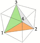
Figure 2: The tetrahedron, with labelled vertices.

We can parameterize matrices in $SU(2)$ in a very similar way: take any unit vector $\hat{n}$, and any angle $-2\pi<\theta\leq 2\pi)$. Notice how $\theta$ runs over a larger range than in the $SO(3)$ case, we now have a sphere with radius $2\pi$ and the surface of the sphere corresponds to the center element $-1$). Now associate to $\hat{n}$ and $\theta$ the following matrix in $SU(2)$:

$$u(\hat{n},\theta)=exp(i\frac{\theta}{2}\hat{n}\cdot\vec{\sigma})=cos(\frac{\theta}{2})\textbf{1}+isin(\frac{\theta}{2})\hat{n}\cdot\vec{\sigma}$$ (36)

where $\vec{\sigma}=(\sigma_{x},\sigma_{y},\sigma_{z})$ is a vector containing the three Pauli matrices, and 1 is the unit matrix.

$$\sigma_{x}=\left(\begin{array}[]{cc}0&1\\ 1&0\end{array}\right),\sigma_{y}=\left(\begin{array}[]{cc}0&-i\\ i&0\end{array}\right),\sigma_{z}=\left(\begin{array}[]{cc}1&0\\ 0&-1\end{array}\right)$$ (37)

The homomorphism $\rho:SU(2)\mapsto SO(3)$ is now easily accomplished: replace $u$ by $R$.

In the achiral tetrahedral phase, the magnetic group is $\tilde{T}$:

$$\Pi_{1}(O(3)/T_{d})=\Pi_{1}(SO(3)/T)=\Pi_{1}(SU(2)/\tilde{T})\simeq\tilde{T}.$$

$\tilde{T}$ is the inverse under $\rho$ of $T$, the tetrahedral group in $SO(3)$. Global symmetry transformations act on the defects in $\tilde{T}$, so the defects are grouped together in orbits under the action of the electric group, in this case $T_{d}$. We note that this is not the same as the conjugacy classes of $\tilde{T}$! To see this, we must first fix a notation for the defects. Write an element of $\tilde{T}$ as

$$u(\hat{n},\theta)=sgn(cos\frac{\theta}{2})u^{\prime}(\hat{n},\theta^{\prime}) -\pi<\theta^{\prime}\leq\pi$$ (38)

$$\theta^{\prime}=\theta(mod2\pi).$$

Every defect corresponds to a $u(\hat{n},\theta)$ (the endpoint of the path in $SU(2)$ that characterizes the defect). We denote the defects as cycles of $T$ with square brackets with a plus or minus sign, e.g. $\pm[123]$. The minus sign corresponds to the $2\pi$ defect, i.e. the nontrivial loop in $SO(3)$. The defect $[123]$ corresponds to the $u^{\prime}(\hat{n},\theta^{\prime})$ with $-\pi<\theta^{\prime}\leq\pi$ such that

$$R(\hat{n},\theta^{\prime})=(123).$$

We need to know the axis $\hat{n_{1}}$ in figure 2, such that $(123)$ corresponds to a $\frac{2\pi}{3}$ rotation around $\hat{n_{1}}$.

From the figure we see that $\hat{n_{1}}=\frac{1}{\sqrt{3}}(1,1,1).$ Thus we define $[123]=u(\hat{n_{1}},\frac{2\pi}{3})$. The trivial defect is denoted by $1$, and the $2\pi$ defect by $-1$.

Preferred element $g_{A}$	Conjugacy class $A$
$\pm e$	$C_{\pm e}=\pm\{e\}$
$\pm[123]$	$C_{\pm[123]}=$
	$\pm\{[123],[134],[142],[243]\}$
$\pm[124]$	$C_{\pm[124]}=$
	$\pm\{[124],[132],[234],[143]\}$
$[(12)(34)]$	$C_{[(12)(34)]}=$
	$\{\pm[(12)(34)],\pm[(13)(24)],$
	$\pm[(14)(23)]\}$

Table 1: The conjugacy classes of $\tilde{T}$, and the preferred elements $g_{A}$. When we write $\pm$ in front of a class, we mean that there are two classes, one with plus signs in front of all the elements, and one with minus signs in front of all the elements. On the other hand, if we write $\pm$ in front of an element inside a class, we mean that the both the element with a plus and minus sign in front of it are present in the class.

To have a notation for all the defects in $\tilde{T}$, we first define the following axes:

$$\hat{n_{1}}=\frac{1}{\sqrt{3}}(1,1,1) \hat{n_{2}}=\frac{1}{\sqrt{3}}(1,1,-1)$$

$$\hat{n_{3}}=\frac{1}{\sqrt{3}}(-1,1,1) \hat{n_{4}}=\frac{1}{\sqrt{3}}(-1,1,-1).$$

Then the defects are given by $\pm e$ and

$$\pm[123]=\pm u(\hat{n_{1}},\frac{2\pi}{3}) \pm[124]=\pm u(\hat{n_{2}},\frac{2\pi}{3})$$

$$\pm[124]=\pm u(\hat{n_{2}},\frac{2\pi}{3}) \pm[234]=\pm u(\hat{n_{3}},\frac{2\pi}{3})$$

$$\pm[134]=\pm u(\hat{n_{4}},\frac{2\pi}{3}) \pm[132]=\pm u(\hat{n_{1}},-\frac{2\pi}{3})$$

$$\pm[142]=\pm u(\hat{n_{2}},-\frac{2\pi}{3}) \pm[243]=\pm u(\hat{n_{3}},-\frac{2\pi}{3})$$

$$\pm[143]=\pm u(\hat{n_{4}},-\frac{2\pi}{3}) \pm[(12)(34)]=\pm u(\hat{z},\pi)$$

$$\pm[(13)(24)]=\pm u(\hat{y},\pi) \pm[(14)(23)]=\pm u(\hat{x},\pi).$$

Using our notation, we can determine the defect classes under the action of $T_{d}$. First consider an element $R(\hat{n},\phi)$ of $T$. Its action on a defect $u(\hat{n_{i}},\theta)$ gives $u(\hat{n},\phi)u(\hat{n_{i}},\theta)u(\hat{n},\phi)^{-1}$.

Classes of $\tilde{T}$ under the action of $T_{d}$
$C_{e}$
$C_{-e}$
$C_{[123]}\cup C_{[124]}$
$C_{-[123]}\cup C_{-[124]}$
$C_{[(12)(34)]}$

Table 2: The defect classes in a theory with $T_{d}$ symmetry. The classes are unions of conjugacy classes of $\tilde{T}$. The conjugacy classes of $\tilde{T}$ are defined in table 1.

Now consider transformations in $T_{d}$ that are not connected to the identity, such as the element $(12)$. These are called “large” symmetry transformations. We can always write a large symmetry transformation as $Inv\times R(\hat{n},\phi)$, where $Inv$ is the inversion matrix:

$$Inv=-\textbf{1}=\left(\begin{array}[]{ccc}-1&0&0\\ 0&-1&0\\ 0&0&-1\end{array}\right).$$ (39)

$Inv$ acts trivially on all the defects, thus the action of $Inv\times R(\hat{n},\phi)$ on a defect $u(\hat{n_{i}},\theta)$ gives $u(\hat{n},\phi)u(\hat{n_{i}},\theta)u(\hat{n},\phi)^{-1}$.

We will now write the large symmetry transformations as $Inv\times R(\hat{n},\phi)$. First we define the following axes:

$$\hat{m}_{1}=\frac{1}{\sqrt{2}}(1,-1,0)\quad\hat{m}_{2}=\frac{1}{\sqrt{2}}(-1,0,1)$$

$$\hat{m}_{3}=\frac{1}{\sqrt{2}}(0,1,1)\quad\hat{m}_{4}=\frac{1}{\sqrt{2}}(0,-1,1)$$

$$\hat{m}_{5}=\frac{1}{\sqrt{2}}(1,0,1)\quad\hat{m}_{6}=\frac{1}{\sqrt{2}}(1,1,0).$$

The inversions are given by

$$(12)=Inv\times R(\hat{m}_{1},\pi) (13)=Inv\times R(\hat{m}_{2},\pi)$$

$$(14)=Inv\times R(\hat{m}_{3},\pi) (23)=Inv\times R(\hat{m}_{4},\pi)$$

$$(24)=Inv\times R(\hat{m}_{5},\pi) (34)=Inv\times R(\hat{m}_{6},\pi).$$

We can now derive the multiplication table of $\tilde{T}$ using the multiplication in $SU(2)$. For example,

$$[123][123]=-[132]$$

$$[123][124]=[(14)(23)]$$

$$(12)[(12)(34)](12)=-[(12)(34)]$$

etc.

The Hopf symmetry of the achiral tetrahedral nematic is the modified quantum double $F(\tilde{T})\times\mathbb{C}T_{d}$. We just defined the action of $T_{d}$ on $\tilde{T}$, which sets the multiplicative structure of $F(\tilde{T})\times\mathbb{C}T_{d}$.

Now that we have elucidated the action of $H_{el}$ on $H_{m}$, we can determine the defect classes. These defect classes are the union of conjugacy classes of $\tilde{T}$. The conjugacy classes of $\tilde{T}$ are shown in table 1, and the defect classes in table 2. The “small” symmetry transformations (that are connected to the identity) simply conjugate the defects, while the large symmetry transformations may transform defects in different conjugacy classes into each other.

$g_{\mathcal{O}}$	Centralizer $N_{\mathcal{O}}$	Irreps
$\pm e$	$T$	$\Pi^{e}_{\alpha}$
$\pm[123]$	$\{e,(123),(132)\}\simeq\mathbb{Z}_{3}$	$\Pi^{\pm[123]}_{k}$, $k\in\mathbb{Z}_{3}$
$\pm[124]$	$\{e,(124),(142)\}\simeq\mathbb{Z}_{3}$	$\Pi^{\pm[124]}_{k}$, $k\in\mathbb{Z}_{3}$
$[(12)(34)]$	$\{e,(12)(34),(13)(24),(14)(23)\}$	$\Pi^{\pm[123]}_{k},k\in\mathbb{Z}_{4}$
	$\simeq\mathbb{Z}_{4}$

Table 3: The irreps of $F(\tilde{T})\times\mathbb{C}T_{d}$. The $\alpha$ are irreps of $T_{d}$.

The centralizers and irreps of $F(\tilde{T})\times\mathbb{C}T_{d}$ are given in table 3.

We must carefully interpret the result that defect classes can be larger than conjugacy classes. The defects in the same class have the same energy, since the symmetry transformations commute with the Hamiltonian. They also have isomorphic centralizers. However, the cores of defects only related by a large symmetry cannot be interchanged. This is due to the fact that the symmetry isn’t connected to the identity. Thus these defects are not topologically equivalent: they cannot be deformed into each other with a finite amount of energy. So we might conclude that we shouldn’t act with large symmetries on the defects, and we should work with conjugacy classes. However, we cannot simply neglect the large global symmetries, since they act on the electric modes.

Finally, we need a map $\Gamma$ from $H_{m}$ to $H_{el}$ to define a braiding (see above): $\Gamma$ is given by

$$\Gamma(\pm[123])=(123),\Gamma(\pm[(12)(34)])=(12)(34),etc.$$

Thus $\Gamma$ turns square brackets into round brackets and neglects the eventual minus sign.

Pref. el. $g_{A}$	Defect class $A$ of $\tilde{O}$
$\pm e$	$C_{\pm e}=\{\pm e\}$
$\pm[123]$	$C_{\pm[123]}=\pm\{[123],[124],[142],[132],[134],$
	$[234],[142],[143],[243]\}$
$\pm[1234]$	$C_{\pm[1234]}=\pm\{[1234],[1243],[1324],$
	$[1342],[1423],[1432]\}$
$[(12)(34)]$	$C_{[(12)(34)]}=\{\pm[(12)(34)],\pm[(13)(24)],\pm[(14)(23)]\}$
$[12]$	$C_{[12]}=\{\pm[12],\pm[13],\pm[23],\pm[14],\pm[24],\pm[34]\}$

Table 4: The defect classes of $\tilde{O}$ under the action $O_{i}$, and the preferred elements $g_{A}$. See 1 for a description of the notation.

Achiral octahedral nematic

The electric group is $O_{i}$, which is the octahedral group $O$ (consisting of the rotational symmetries of a cube), plus the inversions and reflections of a cube. $O$ is isomorphic to $S_{4}$ (all permutations of the diagonals of a cube). Thus we can write elements of $O$ as cycles, e.g. $(1234),(123),(23),(13)(24)$, etc. Defining $Inv$ as in equation (39), we have that $O_{i}=\{O,Inv\times O\}$. Thus elements of $O_{i}$ are (1234), (123), Inv, $Inv\times(134)$, etc.

In analogy with the achiral tetrahedral nematic discussed above, we can denote elements of the magnetic group $\tilde{O}$ as cycles with square brackets, with an eventual minus sign. Examples are $\pm[123],\pm[(12)(34)],\pm[(12)]$, where the minus sign is the $2\pi$ defect.

The Hopf symmetry is $F(\tilde{O})\times CO_{i}$. The defect classes in $\tilde{O}$ under the action of $O_{i}$ are given in table 4. The inversion $Inv$ acts trivially on the defects, so for the octahedral nematic the defect classes are in fact the conjugacy classes of $\tilde{O}$. In general, when a group carries a sublabel $i$, it means that the group contains $Inv$.

Pr. el. $g_{A}$	Defect class $A$ of $\tilde{I}$
$\pm e$	$C_{\pm e}=\pm\{e\}$
$\pm[123]$	$C_{\pm[123]}=\pm\{[123],[132],[124],[142],[125],$
	$[152],[134],[143],[135],[153],$
	$[145],[154],[234],[243],[235],$
	$[253],[245],[254],[345],[354]\}$
$\pm[12345]$	$C_{\pm[12345]}=\pm\{[12345],[12453],[12534],[13254],$
	$[13425],[13542],[14235],[14352],$
	$[14523],[15243],[15324],[15432]\}$
$\pm[12354]$	$C_{\pm[12354]}=\pm\{[12354],[12435],[12543],[13245],$
	$[13452],[13524],[14253],[14325],$
	$[14532],[15234],[15342],[15423]\}$
$[(12)(34)]$	$C_{[(12)(34)]}=$
	$\{\pm[(12)(34)],\pm[(12)(35)],\pm[(12)(45)],\pm[(13)(24)],$
	$\pm[(13)(25)],\pm[(13)(45)],\pm[(23)(45)],\pm[(14)(23)],$
	$\pm[(14)(25)],\pm[(14)(35)],\pm[(24)(35)],\pm[(15)(23)],$
	$\pm[(15)(24)],\pm[(15)(34)],\pm[(25)(34)]\}$
$\pm[123]$	$C_{\pm[123]}=\pm\{[123],[124],[125],[132],[134],$
	$[234],[135],[235],[142],[143],$
	$[243],[145],[245],[345],[152],$
	$[153],[253],[154],[254],[354]\}$

Table 5: The defect classes of $\tilde{I}$ under the action $I_{i}$, and the preferred elements $g_{A}$. See table 1 for a description of the notation.

Achiral icosahedral nematic

The electric group is $I_{i}$, which consists of the icosahedral group $I$ (the rotational symmetries of an icosahedron), plus inversions and reflections of the icosahedron. $I$ is isomorphic to $A_{5}$ (the even permutations of the five cubes inscribed inside an icosahedron). Thus we write elements of $I$ as cycles, e.g. (12345), (14)(23), etc. Just as in the octahedral case, $I_{i}=\{I,Inv\times I\}$.

We can denote elements of the magnetic group $\tilde{I}$ as cycles with square brackets, with an eventual minus sign. Examples are $\pm[123],\pm[(12)(345)],\pm[(15)]$, where the minus sign is the $2\pi$ defect. The Hopf symmetry is $F(\tilde{I})\times\mathbb{C}I_{i}$. The defect classes in $\tilde{I}$ under the action of $I_{i}$ are given in table 5. The inversion $Inv$ acts trivially on the defects, so the defect classes are the conjugacy classes of $\tilde{I}$.

III Defect condensates and Hopf symmetry breaking

III.1 The Hopf symmetry breaking formalism

Using the Hopf symmetry description of a phase, one can study phase transitions induced by the condensation of any mode, be it electric, magnetic or dyonic. The theory of Hopf symmetry breaking was first proposed by Bais, Schroers and Slingerland Bais:2002pb ; Bais:2002ny . who developed the framework that determines the physics of the broken phase, and applied it to discrete gauge theories. The aim of the present article is to apply this framework to non-Abelian nematics. It turns out that we were physically motivated to alter one step of the framework, namely the definition of the residual symmetry algebra. In this section, we briefly introduce the Hopf symmetry breaking formalism, relying strongly on physical motivation. The mathematics of our approach, which differ slightly from the mathematics in papers just mentioned, are discussed in another paper bmbreaking:2006 .

Classically, a condensate corresponds to a nonzero expectation of some (dis)order parameter field. This nonzero expectation value has certain symmetries, its symmetry group is called the residual symmetry group $H$. The quantum interpretation is that the ground state of the system corresponds to a non-vanishing homogeneous density of particles in some particular state. The residual symmetry operators are the operators that leave that particular state invariant. Whether we are working classically or quantum mechanically, the residual symmetry operators are determined the same way: determine the operators that act trivially on the condensate, which is a vector in some irrep of the original symmetry.

If the original symmetry was a group $G$, it would be easy to define what we mean by the symmetry operators of a vector $|\phi_{0}>$ in an irrep $\Pi$ of $G$, namely operators $h\in G$ that satisfy

$$h\cdot|\phi_{0}>=|\phi_{0}>.$$ (40)

If the original symmetry is a Hopf algebra $\mathcal{A}$, on the other hand, the definition of “residual symmetry operators” is not so trivial. This is discussed in a related paperbmbreaking:2006 : There is a physically very attractive definition of a “residual symmetry operator”: an operator is a residual symmetry operator if its action on a particle state is not affected by the fusion of that particle with the state of the particles in the condensate. This means that if this operator acts on any particle, and that particle fuses with the condensate, then the action of the operator on the particle before and after fusion with the condensate is the same. We have to make a choice at this point: whether the particle fuses with the condensate from the left or the right. This is an important point as we argue elsewherebmbreaking:2006 . Here we choose fusion with the condensate from the right. This leads to the definition of $\mathcal{T}_{r}$, the right residual symmetry algebra, which consists of all symmetry operators in $\mathcal{A}$ whose actions on a state are not affected by fusion of the state with the condensate on the right. $\mathcal{T}_{r}$ is the analog of the residual symmetry group when a group symmetry is spontaneously broken. We note that there are cases where $\mathcal{T}_{r}$ isn’t a Hopf algebra.

Once $\mathcal{T}_{r}$ has been established, we must take a close look at the particles in this broken theory, which we now consider to be the irreps of $\mathcal{T}_{r}$. It turns out that some particle species don’t braid trivially with the condensate. The presence of such particles in the system implies a half-line discontinuity in the condensate, across which the internal state of the condensate jumps, which means that these particles have to be connected to a domain wall. Hence, such particles will be confined. We can similarly determine which particles are unconfined, i.e. braid trivially with the condensate, and (in the cases we’ve worked out) these particles turn out to be the irreps of a new Hopf algebra called the unconfined symmetry algebra which will be denoted as $\mathcal{U}$.

Single defect condensate in
$\mathcal{A}=F(\tilde{T})\times\mathbb{C}T_{d}$	$K$	$\mathcal{T}_{r}$	$\mathcal{U}$
$|-e>$	$\tilde{C_{1}}$	$F(T)\times\mathbb{C}T_{d}$	$F(T)\times\mathbb{C}T_{d}$
$|[123]>$	$\tilde{C_{3}}$	$F(T/C_{3})\times\mathbb{C}C_{3}$	$D(e)$
$|[(12)(34)]>$	$\tilde{C_{2}}$	$F(T/C_{2})\times\mathbb{C}D_{2}$	$D(C_{2})$
$|-[(12)(34)]>$	$\tilde{C_{2}}$	$F(T/C_{2})\times\mathbb{C}D_{2}$	$D(C_{2})$

Table 6: Single defect condensates in a tetrahedral nematic. $\mathcal{A}$ is the original Hopf symmetry, $K$ is the smallest subgroup of $H_{m}$ that contains all the defects $g_{i}$ that are in the condensate, $\mathcal{T}_{r}$ is the residual symmetry algebra, and $\mathcal{U}$ is the unconfined Hopf symmetry.

Thus, in contrast with the conventional symmetry breaking analysis, we have to distinguish two steps in the symmetry breaking: first to the residual symmetry algebra $\mathcal{T}_{r}$, and then to the unconfined symmetry algebra $\mathcal{U}$. One should not make the mistake of believing that $\mathcal{U}$ contains all the information about the broken phase: one might believe that the confined particles should be neglected because they cost an infinite amount of energy to create in a system of infinite extent, since the half-line discontinuity costs a finite amount of energy per unit length. However, the half-line may end on another confined excitation, thus giving rise to a wall of finite length. We call a configuration consisting of confined excitations connected by walls, such that the overall configuration is unconfined, a hadronic composite, in analogy with hadrons in Quantum Chromodynamics, where hadrons are unconfined composites of confined quarks. $\mathcal{T}_{r}$ contains all the information about the hadrons, although it is not trivial to extract this informationbmbreaking:2006 experimentally.

III.2 Defect condensates and residual symmetry algebras

One can derive general formulae for $\mathcal{T}_{r}$ and $\mathcal{U}$ in the case of defect condensates in a phase with $F(H_{m})\times\mathbb{C}H_{el}$ symmetrybmbreaking:2006 . Here we will just summarize the resulting formulae, and in the next section apply them to the classification of all possible defect condensates in achiral tetrahedral, octahedral and icosahedral nematics.

Class sum def. condensate
of $\mathcal{A}=F(\tilde{T})\times\mathbb{C}T_{d}$	$K$	$\mathcal{T}_{r}$	$\mathcal{U}$
$|C_{-e}>$	$\tilde{C_{1}}$	$F(T)\times\mathbb{C}T_{d}$	$F(T)\times\mathbb{C}T_{d}$
$|C_{[123]}>,|C_{-[123]}>,$	$\tilde{T}$	$\mathbb{C}T$	$D(e)$
$\qquad|C_{[124]}>,|C_{-[124]}>$
$|C_{[(12)(34)]}>$	$\tilde{D_{2}}$	$F(\mathbb{Z}_{3})\times\mathbb{C}T_{d}$	$F(\mathbb{Z}_{3})\times\mathbb{C}(\mathbb{Z}_{3})_{d}$

Table 7: Conjugacy class sum defect condensates in an achiral tetrahedral nematic. $(\mathbb{Z}_{3})_{d}$ is isomorphic to the permutation group of 3 elements.

Given a phase with Hopf symmetry $\mathcal{A}=F(H_{m})\times\mathbb{C}H_{el}$, the condensate $|\phi_{0}>$ is a vector in some irrep $\Pi^{A}_{\alpha}$ of $\mathcal{A}$. We must demand that $|\phi_{0}>$ braid trivially with itself, otherwise the condensate is ill-defined (the condensate itself would be filled with half-line singularities). Thus we demand that

$$\mathcal{R}\cdot|\phi_{0}>|\phi_{0}>=|\phi_{0}>|\phi_{0}>.$$ (41)

Now let us take $|\phi_{0}>$ to be a defect condensate, which means it is a vector in a magnetic irrep $\Pi^{A}_{1}$ ($1$ is the trivial irrep of the normalizer $N_{A}$). There are different types of defect condensates which we wish to analyze. A basis of the vector space on which this irrep acts is given by $\{|g^{A}_{i}>\}$, where the $g^{A}_{i}$ are the different defects in $A$. We consider the following types of condensates:

• Single defect condensate

  $$|\phi_{0}>=|g^{A}_{i}>$$ (42)

• Class sum defect condensate

  $$|\phi_{0}>=\sum_{g_{i}\in A}|g_{i}>=:|C_{g_{A}}>$$ (43)

  where $C_{g_{A}}$ is a defect class (i.e. the orbit of $g_{A}$ under the action of $H_{el}$). We denote the condensate by $|C_{g_{A}}>$, where $g_{A}$ is the preferred element of $A$.

• Combined defect condensate

  $$|\phi_{0}>=\sum_{g_{i}\in E}|g_{i}>$$ (44)

  where $E$ is a subset of the defects in one class. We need only take the elements to be within one class because it turns out that we need only study the cases where the condensate is the sum of vectors in the same irrep (all other phase transitions can be interpreted as a sequential condensation of vectors in different irrepsbmbreaking:2006 .).

Combined def. cond.	$K$	$\mathcal{T}_{r}$	$\mathcal{U}$
of $\mathcal{A}=F(\tilde{T})\times\mathbb{C}T_{d}$
$|[123]>+|[132]>$	$\tilde{C_{3}}$	$F(T/C_{3})\times\mathbb{C}C_{3v}$	$\mathbb{C}C_{1v}$
$|[(12)(34)]>+|[(13)(24)]>$	$\tilde{D_{2}}$	$F(T/D_{2})\times\mathbb{C}C_{2v}$	$\mathbb{C}C_{1v}$
$\{|[(12)(34)]>+$	$\tilde{D_{2}}$	$F(T/D_{2})\times\mathbb{C}D_{2d}$	$\mathbb{C}C_{1v}$
$|[-(12)(34)]>+|[(13)(24)]>$
$+|-[(13)(24)]>\}$
$|[(12)(34)]>+|[-(12)(34)]>$	$\tilde{C_{2}}$	$F(T/C_{2})\times\mathbb{C}D_{2d}$	$F(C_{2})$
			$\times\mathbb{C}C_{2v}$
$|[(12)(34)]>+|[(13)(24)]>$	$\tilde{D_{2}}$	$F(\mathbb{Z}_{3})\times\mathbb{C}T$	$D(\mathbb{Z}_{3})$
$\qquad+|[(14)(23)]>$

Table 8: Combined defect condensates in an achiral tetrahedral nematic (that satisfy trivial self braiding). No two defect condensates have simultaneously the same $\mathcal{T}_{r}$ and $\mathcal{U}$. Thus in principle the different defect condensates are distinguishable.

The single defect and class sum defect condensates are a special case of combined defect condensate.

III.2.1 Single defect condensate

Condense $|g_{A}>$ in the magnetic irrep $\Pi^{A}_{1}$. The condensate $|g_{A}>$ satisfies the trivial self braiding condition mentioned above. The residual symmetry algebra is

$$\mathcal{T}_{r}=F(H_{m}/(g_{A}))\otimes\mathbb{C}N_{A}$$ (45)

where we define $(g_{A})$ to be the smallest subgroup of $H_{m}$ that contains $g_{A}$.

This result for $\mathcal{T}_{r}$ has a very natural interpretation: the residual electric group is $N_{A}$, the subgroup of $H$ that doesn’t conjugate the defect. The magnetic part $H/(g_{A})$ is not necessarily a group. It consists of left cosets of $(g_{A})=\{\ldots g_{A}^{-1},e,g_{A},g_{A}^{2},\ldots\}$. The defects are now defined modulo the condensate defect $|g_{A}>$. In other words, if a particle in a magnetic irrep of the residual symmetry $\mathcal{T}_{r}$ fuses with the condensate $|g_{A}>$, it is left unchanged. Thus its topological charge is defined modulo $g_{A}$.

One can prove that $\mathcal{T}_{r}$ is a Hopf algebra $\iff$ $(g_{A})$ is a normal subgroup of $H_{m}$ $\iff$ $H_{m}/(g_{A})$ is a group.

The unconfined symmetry algebra is

$$\mathcal{U}=F(\Gamma^{-1}(N_{A})/(g_{A}))\times\mathbb{C}(N_{A}/\Gamma(g_{A})).$$ (46)

Note that we condensed $|g_{A}>$, where $g_{A}$ was a chosen defect in the defect class $A$. $g_{A}$ was chosen arbitrarily, so our formulae are general.

Single def. cond.
of $\mathcal{A}=F(\tilde{O})\times\mathbb{C}O_{i}$	$K$	$\mathcal{T}_{r}$	$\mathcal{U}$
$|-e>$	$\tilde{C_{1}}$	$F(O)\times\mathbb{C}O_{i}$	$F(O)\times\mathbb{C}O_{i}$
$|\pm[12]>$	$\tilde{C_{2}}$	$F(O/C_{2})\times\mathbb{C}D_{2i}$	$F(C_{2})\times\mathbb{C}C_{2i}$
$|\pm[123]>$	$\tilde{C_{3}}$	$F(O/C_{3})\times\mathbb{C}C_{3i}$	$\mathbb{C}C_{i}$
$|\pm[1234]>$	$\tilde{C_{4}}$	$F(O/C_{4})\times\mathbb{C}C_{4i}$	$\mathbb{C}C_{i}$
$|\pm[(12)(34)]>$	$\tilde{C_{2}}$	$F(O/C_{2})\times\mathbb{C}D_{4i}$	$F(D_{2})\times\mathbb{C}D_{2i}$

Table 9: Single defect condensates in an achiral octahedral nematic. When we write $\pm$ in front of a condensate, we mean that the condensate with or without the minus sign gives the same symmetry breaking analysis.

III.2.2 Class sum defect condensates

Condense the sum of the defects in the defect class $A$:

$$|\phi_{0}>=\sum_{g^{A}_{i}\in A}|g^{A}_{i}>=:|C_{g_{A}}>.$$

A class sum defect condensate satisfies the trivial self braiding condition (41):

$$\mathcal{R}(|C_{g_{A}}> \otimes |C_{g_{A}}>)$$

$$= \mathcal{R}(\sum_{g^{A}_{i}\in A}|g^{A}_{i}>\otimes\sum_{g^{A}_{k}\in A}|g^{A}_{k}>)$$

$$= \sum_{g^{A}_{i}\in A}(\sum_{g^{A}_{k}\in A}|g^{A}_{i}g^{A}_{k}(g^{A}_{i})^{-1}>)\otimes|g^{A}_{i}>$$

$$= \sum_{g^{A}_{i}\in A}(\sum_{g^{A}_{k}\in A}|g^{A}_{k}>)\times|g^{A}_{i}>.$$

$$= |C_{g_{A}}>\otimes|C_{g_{A}}>$$

In going from the second to the third line, we use the fact that $gAg^{-1}=A$ for any $g\in H_{m}$.

Class sum def. cond.
of $\mathcal{A}=F(\tilde{O})\times\mathbb{C}O_{i}$	$K$	$\mathcal{T}_{r}$	$\mathcal{U}$
$|C_{[(12)(34)]}>$	$\tilde{D_{2}}$	$F(D_{3})\times\mathbb{C}O_{i}$	$F(D_{3})\times\mathbb{C}D_{3i}$
$|C_{\pm[123]}>$	$\tilde{T}$	$F(C_{2})\times\mathbb{C}O_{i}$	$F(C_{2})\times\mathbb{C}C_{2i}$
$|C_{\pm[1234]}>$	$\tilde{O}$	$\mathbb{C}O_{i}$	$\mathbb{C}C_{i}$
$|C_{[12]}>$	$\tilde{O}$	$\mathbb{C}O_{i}$	$\mathbb{C}C_{i}$

Table 10: Conjugacy class sum defect condensates in an achiral octahedral nematic. When we write $\pm$ is front of a condensate, we mean that the condensate with or without the minus sign gives the same symmetry breaking analysis.

A class sum condensate doesn’t break the electric group at all! Namely, all elements of $H_{el}$ act trivially on a defect class, since for any $g\in H_{el}$ we have

$$g\cdot|\phi_{0}>=g\cdot(\sum_{g^{A}_{i}\in A}|g^{A}_{i}>) =$$

$$\quad=\sum_{g^{A}_{i}\in A}|g\cdot g^{A}_{i}> = \sum_{g^{A}_{i}\in A}|g^{A}_{i}>=|\phi_{0}>.$$

Thus this condensate is invariant under all of $H_{el}$. For this reason, such a condensate is admissible in a theory where the symmetry is gauged and we call it a gauge invariant magnetic condensate (the condensate respects gauge invariance). In a global theory all condensates are admissible.

The residual and unconfined symmetry algebras are respectively

$$\mathcal{T}_{r}=F(H_{m}/K)\times\mathbb{C}H_{el}$$ (47)

$$\mathcal{U}=F(H_{m}/K)\times\mathbb{C}H_{el}/\Gamma(K),$$ (48)

where $K$ is the smallest subgroup of $H_{m}$ that contains the class $A$. From this definition, one can prove that $K$ is a normal subgroup of $H_{m}$. Thus $H_{m}/K$ is a group, and $\mathcal{T}_{r}$ is a Hopf algebra.

Later on, we will consider conjugacy class sum defect condensates, i.e. condensates of a sum of defects in the same conjugacy class of $H_{m}$. This can be a whole defect class, or it can be smaller than a whole defect class. If it is smaller, then the electric group is partially broken.

III.2.3 Combined defect condensates

Start with a phase with $F(H_{m})\times\mathbb{C}H_{el}$ symmetry. Choose an irrep $\Pi^{A}_{\alpha}$, and consider a condensate of the form $\sum_{g_{i}\in E}|g_{i}>$, with $E$ a subset of the defects in one defect class.

The demand of trivial self braiding (41) gives

$$\mathcal{R}(\sum_{g_{i}\in E}|g_{i}>\otimes\sum_{g_{k}\in E}|g_{k}>) =\sum_{g_{i}\in E}|g_{i}>\otimes\sum_{g_{k}\in E}|g_{k}>$$

$$\iff$$

$$\sum_{g_{k}\in E}\sum_{g_{i}\in E}|g_{i}g_{k}g_{i}^{-1}>\otimes|g_{i}> =\sum_{g_{i}\in E}\sum_{g_{k}\in E}|g_{i}>\otimes|g_{k}>$$

$$\iff$$

$$\forall g_{i}\in E:\{g_{i}g_{k}g_{i}^{-1}\}_{g_{k}\in E} =\{g_{k}\}_{g_{k}\in E}.$$ (49)

It is interesting in itself to study how many different defect condensates satisfy this criterion. Defect-antidefect condensates $|g>+|g^{-1}>$ always satisfy this criterion, as do any set of commuting elements in a certain conjugacy class, and class sum defect condensates. The trivial self braiding condition plays a crucial role in determining $\mathcal{T}_{r}$bmbreaking:2006 .

The results for $\mathcal{T}_{r}$ and $\mathcal{U}$ are:

$$\mathcal{T}_{r}=F(H_{m}/K)\times\mathbb{C}M_{E}$$

$$\mathcal{U}=F(N_{E}/K)\times\mathbb{C}M_{E}/\Gamma(K),$$

where we must still define all the notation in these results.

Combined def. cond.	$K$	$\mathcal{T}_{r}$	$\mathcal{U}$
of $\mathcal{A}=F(\tilde{O})\times\mathbb{C}O_{i}$
$|[123]>+|[132]>$	$\tilde{C_{3}}$	$F(O/C_{3})\times\mathbb{C}D_{3i}$	$\mathbb{C}C_{2i}$
$|[12]>+|[34]>$	$\tilde{D_{2}}$	$F(O/D_{2})\times\mathbb{C}D_{4i}$	$F(C_{2})\times\mathbb{C}C_{i}$
$|[(12)(34)]>\qquad$	$\tilde{D_{2}}$	$F(O/D_{2})\times\mathbb{C}D_{4i}$	$F(C_{2})\times\mathbb{C}C_{2i}$
$\qquad+|[(13)(24)]>$
$|[12]>+|[13]>+|[23]>$	$\tilde{D_{3}}$	$F(O/D_{3})\times\mathbb{C}D_{3i}$	$\mathbb{C}C_{i}$

Table 11: Combined defect condensates in an achiral octahedral nematic.

Define the following subset of $H_{el}$ (which needn’t be a subgroup):

$$V_{E}\subset H_{el}:\;V_{E}=\{x_{i}N_{A}\}_{g_{i}\in E}$$ (50)

where $N_{A}\subset H_{el}$ is the normalizer of the chosen preferred element $g_{A}$ in $A$, and the $x_{i}$ satisfy $x_{i}g_{A}x_{i}^{-1}=g_{i}\in E$. $V_{E}$ corresponds to the set of left $N_{A}$ cosets that corresponds to the defects in the condensate (under a correspondence discussed above).

Define the following subgroup of $H_{el}$:

$$M_{E}\subset H_{el}:\;M_{E} = \{m\in H_{el}:\{m\cdot g_{i}\}_{g_{i}\in E}=\{g_{i}\}_{g_{i}\in E}\}$$ (51)

$$= \{m\in H_{el}:mV_{E}=V_{E}\}.$$

$M_{E}$ is composed of the global symmetry transformations that leave the condensate invariant.

$\mathcal{A}=F(\tilde{I})\times\mathbb{C}I_{i}$	$K$	$\mathcal{T}_{r}$	$\mathcal{U}$
$|-e>$	$\tilde{C_{1}}$	$F(I)\times\mathbb{C}I_{i}$	$F(I)\times\mathbb{C}I_{i}$
$|[123]>$	$\tilde{C_{3}}$	$F(I/C_{3})\times\mathbb{C}C_{3i}$	$\mathbb{C}C_{i}$
$|-[123]>$	$C_{3}$	$F(\tilde{I}/C_{3})\times\mathbb{C}C_{3i}$	$\mathbb{C}C_{i}$
$|\pm[(12)(34)]>$	$\tilde{C_{2}}$	$F(I/C_{2})\times\mathbb{C}D_{2i}$	$F(C_{2})\times\mathbb{C}C_{2i}$
$|[12345]>$	$\tilde{C_{5}}$	$F(I/C_{5})\times\mathbb{C}C_{5i}$	$\mathbb{C}C_{i}$
$|-[12345]>$	$C_{5}$	$F(\tilde{I}/C_{5})\times\mathbb{C}C_{5i}$	$\mathbb{C}C_{i}$

Table 12: Single defect condensates in an achiral icosahedral nematic.

Also define

$$N_{E}\subset H_{m}:\;N_{E}=\{n\in H_{m}:\{ng_{i}n^{-1}\}_{g_{i}\in E}=\{g_{i}\}_{g_{i}\in E}\}.$$

Using (32): $\Gamma(g_{1})\cdot g_{2}=g_{1}g_{2}g_{1}^{-1}\;\forall g_{1},g_{2}\in H_{m}$, we can prove that

$$\Gamma^{-1}(M_{E})=N_{E}\quad\textrm{and}\quad\Gamma(N_{E})=M_{E}.$$ (52)

Finally, we need one more definition:

$$K\subset H_{m}:\;K=(\{g_{i}\}_{g_{i}\in E}),$$ (53)

where $(\{g_{i}\}_{g_{i}\in E})$ is the smallest subgroup of $H_{m}$ that contains all the $g_{i}\in E$, i.e. the defects in the condensate.

The trivial self braiding equation (49) implies that $K\subset N_{E}$. Thus, according to (52) and (50)

$$\Gamma(K)\subset M_{E}.$$ (54)

Summarizing, the unconfined magnetic group is $N_{E}/K$, and the unconfined electric irreps are those that have $\Gamma(K)$ in their kernel, which means that the electric group is $M_{E}/\Gamma(K)$. If we take a quantum double $D(H)$ ($H=H_{el}=H_{m}$), the unconfined symmetry algebra becomes $\mathcal{U}=D(N_{E}/K)$, because in that case $M_{E}=N_{E}$.

III.3 Non-Abelian condensates in liquid crystals

We are now in a position to apply the results obtained in the previous sections to the case of non-Abelian nematics. We have worked out pretty much exhaustive listings of all possible phases characterized by defect condensates in achiral tetrahedral, octahedral and icosahedral nematics. In the corresponding tables of defect condensates we give, $\mathcal{A}$ is the original Hopf symmetry, $K$ is the smallest subgroup of $H_{m}$ that contains all the defects $g_{i}$ that are in the condensate, $\mathcal{T}_{r}$ is the residual symmetry algebra, and $\mathcal{U}$ is the unconfined Hopf symmetry. The defect condensates satisfy trivial self braiding, as we required above.

By looking at all the tables of defect condensates in this section, we note that two different condensates in our tables never give simultaneously the same $\mathcal{T}_{r}$ and $\mathcal{U}$. Some condensates give the same unconfined symmetry algebra, but $\mathcal{T}_{r}$ is then different. Thus there are differences in the spectrum, though these are often hidden in the unconfined spectrum of the hadrons corresponding to different condensates. These differences are therefore quite subtle and may be hard to detect but in principle they are distinguishable. The problem with measuring defect condensates, for example, is that the conventional measuring techniques can measure the electric symmetry group (by looking at Bragg reflections, for example), but as far as we know there are no techniques yet to measure the magnetic symmetry group. Naively this amounts to identifying the surviving unconfined degrees of freedom and their interactions, for example by certain interference experiments. We would need to measure non-Abelian statistics to probe the braiding properties of the particles in the broken phase. Only recently have there been direct measurements of fractional statistics Camino . Nevertheless, if suitable techniques were developed, then we could use our tables to identify a plethora of new phases and determine which condensates they correspond to.

$\mathcal{A}=F(\tilde{I})\times\mathbb{C}I_{i}$	$K$	$\mathcal{T}_{r}$	$\mathcal{U}$
$|C_{\pm[12345]}>$	$\tilde{I}$	$\mathbb{C}I_{i}$	$\mathbb{C}C_{i}$
$|C_{\pm[12354]}>$	$\tilde{I}$	$\mathbb{C}I_{i}$	$\mathbb{C}C_{i}$
$|C_{[(12)(34)]}>$	$\tilde{I}$	$\mathbb{C}I_{i}$	$\mathbb{C}C_{i}$

Table 13: Conjugacy class sum defect condensates in an achiral icosahedral nematic.

III.3.1 Achiral tetrahedral nematic

We have listed all defect condensates in an achiral tetrahedral nematic: the single defect condensates are collected in table 6, the class sum condensates in table 7, and the combined defect condensates in table 8 .

III.3.2 Achiral octahedral nematic

The single defect condensates breaking $F(\tilde{O})\times\mathbb{C}O_{i}$ are given in table 9. The class sum defect condensates are given in table 10. Finally, the combined defect condensates are given in table 11. We note that the list presented here is very representative. The other conceivable defect condensates give the same $\mathcal{T}_{r}$ and $\mathcal{U}$ as one of the defect condensates shown here (except for a small difference: there may be condensates where $K$ is actually the double of a $K$ given here. That slightly changes the magnetic part of $\mathcal{T}_{r}$, but doesn’t affect $\mathcal{U}$). These other defect condensates are trivially different from the ones in the table: for example, they may be permutations of the of the numbers used in the naming of the defects.

$\mathcal{A}=F(\tilde{I})\times\mathbb{C}I_{i}$	$K$	$\mathcal{T}_{r}$	$\mathcal{U}$
$|[(12)(34)]>+|[(13)(24)]>$	$\tilde{D_{2}}$	$F(I/D_{2})\times\mathbb{C}D_{2i}$	$\mathbb{C}C_{i}$
$|[(12)(34)]+|[(13)(24)]>+$	$\tilde{D_{2}}$	$F(I/D_{2})\times\mathbb{C}T_{i}$	$\mathbb{C}C_{3i}$
$\qquad+|[(14)(23)]>$
$|[(12)(34)]>+|[(12)(35)]>+$	$\tilde{D_{3}}$	$F(I/D_{3})\times\mathbb{C}D_{3i}$	$\mathbb{C}C_{i}$
$\qquad+|[(12)(45)]>$
$\{|[(12)(34)]>+|[(13)(25)]>+$	$\tilde{D_{5}}$	$F(I/D_{5})\times\mathbb{C}D_{5i}$	$\mathbb{C}C_{2i}$
$+|[(15)(24)]>+|[(23)(45)]>$
$\qquad+|[(14)(35)]>\}$
$|[123]>+|[132]>$
	$\tilde{C_{3}}$	$F(I/C_{3})\times\mathbb{C}D_{3i}$	$\mathbb{C}C_{2i}$
$|[123]>+|[134]>+$	$\tilde{T}$	$F(I/T)\times\mathbb{C}T_{i}$	$\mathbb{C}C_{i}$
$\qquad+|[142]>+|[243]>$
$\{|[123]>+|[124]>+$	$\tilde{T}$	$F(I/T)\times\mathbb{C}T_{i}$	$\mathbb{C}C_{i}$
$\qquad+|[132]>+|[134]>+$
$+|[234]>+|[142]>+$
$\qquad+|[143]>+|[243]>\}$
$\{|[123]>+|[152]>+$	$\tilde{I}$	$\mathbb{C}C_{3i}$	$\mathbb{C}C_{i}$
$\qquad+|[135]>+|[253]>+$
$+|[142]>+|[134]>+$
$\qquad+|[243]>\}$
$\{|[12345]>+|[13524]>$	$\tilde{C_{5}}$	$F(I/C_{5})\times\mathbb{C}D_{5i}$	$\mathbb{C}C_{2i}$
$+|[14253]>+|[15432]>\}$

Table 14: Combined defect condensates in an achiral icosahedral nematic.

III.3.3 Achiral icosahedral nematic

The single defect condensates in $F(\tilde{I})\times\mathbb{C}I_{i}$ are given in table 12. The class sum defect condensates are given in table 13. Finally, the combined defect condensates are given in table 14. The sample we present in the table is basically exhaustive.

III.3.4 Comments on the conjectured phases

The tables given above, containing the possible phases induced by defect condensation yield a lot of information of both physical and mathematical interest. Yet, they don’t tell the full story, as they do not describe the hadronic composites which we alluded to earlier. Information on these composites is laborious but straightforward to extract, and we would like to comment on what kind of analysis would reveal the hadronic content of a particular phase.

First we note that more often than not, the residual symmetry algebra $\mathcal{T}_{r}$ is not a Hopf algebra . This is perfectly acceptable, since there is no physical reason to assume that $\mathcal{T}_{r}$ is a Hopf algebra. The reason is subtle bmbreaking:2006 : for a symmetry algebra to be a Hopf algebra, it is necessary that the fusion of particles (i.e. the tensor product of irreducible representations) be associative. Now some of the irreducible representations of $\mathcal{T}_{r}$ correspond to confined excitations, which means that the condensate is in a different internal state to the left and right of the excitation. Thus particles to the left of this confined excitation “see” a different condensate. This leads to the necessity of introducing an ordering when taking the tensor product of representations, which corresponds to specifying in which order the particles are brought into the system.

The unconfined symmetry algebra $\mathcal{U}$ corresponds to the symmetry algebra whose irreducible representations are precisely the unconfined representations of $\mathcal{T}_{r}$. These unconfined representations don’t suffer from the necessity of introducing an order, and therefore we expect $\mathcal{U}$ to be a Hopf algebra. In all the cases we’ve worked out this turns out to be the case.

From the tables we learn that different defect condensates may induce the same $\mathcal{U}$, however, they do lead to a different $(\mathcal{T}_{r},\mathcal{U})$ pair. If two phases have the same $\mathcal{U}$, their low energy degrees of freedom share many properties (e.g. their representation theory, their braiding properties). So to tell these two phases apart, it may be necessary to probe unconfined composites of confined excitations (which we called hadronic composites). These may occur at a higher energy scale (depending on the precise dynamics). The constituent structure of the hadronic composites can be derived from $\mathcal{T}_{r}$. To determine the admissible composites, one must take tensor products of several confined excitations and decompose the product into a direct sum of irreducible representations. Every unconfined representation that appears in such a decomposition, corresponds to a hadronic composite. Note that even if $\mathcal{U}=\mathbb{C}e$, the trivial Hopf algebra, there can still be nontrivial composites, the decomposition then has to yield the trivial representation (of $\mathcal{T}_{r}$). It is rather tedious to work out the sets of simplest allowed composites, because the calculation is complicated by the fact that $\mathcal{T}_{r}$ is not a Hopf algebra, but it is straightforward. We have refrained from carrying out such an analysis at this stage.

IV Conclusions

In this paper we have applied the formalism for breaking quantum double symmetries by defect condensates to some classes of rather exotic non-Abelian nematics. We found a wide variety of conceivable phases each characterized by a set of unconfined degrees of freedom associated with an unconfined algebra $\mathcal{U}$. There may also be confined degrees of freedom described by an intermediate symmetry algebra $\mathcal{T}_{r}$. Clearly, whether such phases will actually be realized in nature depends on the detailed dynamics of these media. It would of course be of great value to look for experimental parameters by which these phases could be induced and furthermore to develop observable signatures by which they could be distinguished. These important questions deserve serious attention but are beyond the kinematical scope of this paper.
Acknowledgement: One of us (F.A.B.) likes to thank the Yukawa Institute for Theoretical Physics of Kyoto University for an inspiring visit during which part of this work was carried out.

References

- [1] F. A. Bais, B. J. Schroers, and J. K. Slingerland. Broken quantum symmetry and confinement phases in planar physics. Phys. Rev. Lett., 89:181601, 2002.
- [2] F. A. Bais, B. J. Schroers, and J. K. Slingerland. Hopf symmetry breaking and confinement in (2+1)-dimensional gauge theory. JHEP, 05:068, 2003.
- [3] F.A. Bais and C.J.M. Mathy. The breaking of quantum double symmetries by defect condensation. arXiv:cond-mat/0602115, 2006.
- [4] T.C. Lubensky and L. Radzihovsky. Theory of bent-core liquid-crystal phases and phase transitions. Phys. Rev. E 66, 031704, 2002.
- [5] E. Fradkin and S.A. Kivelson. Liquid-crystal phases of quantum Hall systems. Phys. Rev. B, 59(12):8065–8072, 1999.
- [6] L. Radzihovsky and A.T. Dorsey. Theory of Quantum Hall Nematics. Phys. Rev. Lett., 88(21):216802, 2002.
- [7] Z. Nussinov J. Zaanen and S.I. Mukhin. Duality in 2+1D Quantum Elasticity: superconductivity and Quantum Nematic Order. Ann. Phys., 310:181, 2004.
- [8] P. Chandra and P. Coleman. Quantum spin nematics: Moment-free magnetism. Phys. Rev. Lett., 66:100–103, 1991.
- [9] J. Zaanen and Z. Nussinov. Stripe fractionalization: the quantum spin nematic and the Abrikosov lattice. Physica Status Solidi (b), 236:332–339, 2003.
- [10] P.G. de Gennes and P.J. Prost. The Physics of Liquid Crystals. Oxford Science Publications, second edition edition, 1993.
- [11] N.D. Mermin. Topological theory of defects in ordered media. Rev. Mod. Phys. 51, 591, 1979.
- [12] P.M. Chaikin and T.C. Lubensky. Principles of condensed matter physics. Cambridge University Press, 1995.
- [13] P.H. Butler. Point group symmetry applications. Plenum Press, New York, 1981.
- [14] F.A. Bais and C.J.M. Mathy. Defect mediated melting and the breaking of quantum double symmetries. arXiv:cond-mat/0602101, 2006.
- [15] F.A. Bais. Flux metamorphosis. Nucl. Phys. B, 170:32–43, 1980.
- [16] M. de Wild Propitius and F. A. Bais. Discrete gauge theories. In G. Semenoff and L. Vinet, editors, Particles and Fields, CRM Series in Mathematical Physics, pages 353–439, New York, 1998. Springer Verlag.
- [17] H.K.-Lo and J. Preskill. Non-abelian vortices and non-abelian statistics. Phys. Rev. D, 48(10):4821–4835, 1993.
- [18] F. A. Bais and J. Striet. Charge instabilities due to local charge conjugation symmetry in (2+1)-dimensions. Nucl. Phys., B666:243–268, 2003.
- [19] P. McGraw. Global analogue of Cheshire charge. Phys. Rev. D, 50:952–961, 1994.
- [20] A.P. Balachandran, F. Lizzi, and V.G.J. Rodgers. Topological symmetry breakdown in cholesterics, nematics and helium 3. Phys. Rev. Lett., 52(20):1818–1821, 1984.
- [21] R. Dijkgraaf, V. Pasquier, and P. Roche. Quasi Hopf Algebras, Group Cohomology and Orbifold Models. Nucl. Phys. B (Proc. Suppl.), 18B:60–72, 1990.
- [22] V. Poenaru and G. Toulouse. The crossing of defects in ordered media and the topology of 3-manifolds. J. Phys. (Paris), 8:1405, 1977.
- [23] J. March-Russell, J. Preskill, and F. Wilczek. Internal frame dragging and a global analogue of the Aharonov-Bohm effect. Phys. Rev. Lett., 68:2567, 1992.
- [24] M.O. Katanaev. Geometric theory of defects. PHYS-USP, 48 (7):675–701, 2005.
- [25] H. Kleinert. Gauge fields in Condensed Matter, Vol. I: Superflow and Vortex Lines, Disorder Fields, Phase Transitions. world scientific, Singapore, 1989.
- [26] M.V. Khazan. Analog of the Aharonov-Bohm effect in superfluid . JETP Lett., 41:486, 1985.
- [27] Wei Zhou F.E. Camino and V.J. Goldman. Realization of a Laughlin quasiparticle interferometer: Observation of fractional statistics. Phys. Rev. B., 72:075342, 2005.
- [28] S. Majid. Foundations of Quantum Group Theory. Cambridge University Press, 1995.