Feedback-optimized parallel tempering Monte Carlo

Abstract

We introduce an algorithm to systematically improve the efficiency of parallel tempering Monte Carlo simulations by optimizing the simulated temperature set. Our approach is closely related to a recently introduced adaptive algorithm that optimizes the simulated statistical ensemble in generalized broad-histogram Monte Carlo simulations. Conventionally, a temperature set is chosen in such a way that the acceptance rates for replica swaps between adjacent temperatures are independent of the temperature and large enough to ensure frequent swaps. In this paper, we show that by choosing the temperatures with a modified version of the optimized ensemble feedback method we can minimize the round-trip times between the lowest and highest temperatures which effectively increases the efficiency of the parallel tempering algorithm. In particular, the density of temperatures in the optimized temperature set increases at the “bottlenecks” of the simulation, such as phase transitions. In turn, the acceptance rates are now temperature dependent in the optimized temperature ensemble. We illustrate the feedback-optimized parallel tempering algorithm by studying the two-dimensional Ising ferromagnet and the two-dimensional fully-frustrated Ising model, and briefly discuss possible feedback schemes for systems that require configurational averages, such as spin glasses.

I Introduction

The free energy landscapes of complex systems are characterized by many local minima that are separated by entropic barriers. The simulation of such systems with conventional Monte Carlo methods is slowed down by long relaxation times due to the suppressed tunneling through these barriers. Extended ensemble simulations address this problem by broadening the range of phase space which is sampled in the respective reaction coordinate. Recently, an adaptive algorithm Trebst et al. (2004) has been introduced that explores entropic barriers by sampling a broad histogram in a reaction coordinate and iteratively optimizes the simulated statistical ensemble defined in the reaction coordinate to speed up equilibration. The key idea of the approach is to measure the local diffusivity along the reaction coordinate, thereby identifying the bottlenecks in the simulations and then using this information to systematically shift statistical weights towards these bottlenecks in a feedback loop. The optimized histogram converges to a characteristic form exhibiting peaks at the bottlenecks of the simulation, e.g., in the vicinity of the entropic barriers. The simulation of an optimized ensemble results in equilibration times that can be substantially lower compared to other extended ensemble simulations that aim at sampling a flat histogram in the respective reaction coordinate Trebst et al. (2004); Dayal et al. (2004). Flat-histogram algorithms include the multicanonical method Berg and Neuhaus (1991, 1992), broad histograms de Oliveira et al. (1996) and transition matrix Monte Carlo Wang and Swendsen (2002) when combined with entropic sampling, as well as the adaptive algorithm of Wang and Landau Wang and Landau (2001a, b).

Parallel tempering Monte Carlo Hukushima and Nemoto (1996) has proven to be a strong “workhorse” in fields as diverse as chemistry, physics, biology, engineering, and material science Earl and Deem (2005). Similar to replica Monte Carlo Swendsen and Wang (1986), simulated tempering Marinari and Parisi (1992), or extended ensemble methods Lyubartsev et al. (1992), the algorithm aims to overcome entropic barriers in the free energy landscape by simulating a broad range of temperatures. This allows the system to escape metastable states when wandering to higher temperatures and subsequently relaxing at lower temperatures again on time scales that are substantially smaller than conventional simulations at a fixed temperature. In this paper, we maximize the efficiency of parallel tempering Monte Carlo by optimizing the distribution of temperature points in the simulated temperature set such that round-trip rates of replicas between the two extremal temperatures in the simulated temperature set are maximized. The optimized temperature sets are determined by an iterative feedback algorithm that is closely related to the previously mentioned adaptive ensemble optimization method for broad-histogram Monte Carlo simulations Trebst et al. (2004). The feedback method concentrates temperature points near the bottleneck of a simulation, typically in the vicinity of a phase transition or the ground state of the system. As a consequence, we find that for the optimal choice of temperatures the acceptance probabilities for swap moves between neighboring temperature points show a strong modulation with temperature and are not independent of temperature as suggested in several recent approaches Kofke (2004a, b); Rathore et al. (2005); Predescu et al. (2004, 2005); Kone and Kofke (2005).

The paper is structured as follows: In Sec. II we present a detailed introduction of the parallel tempering Monte Carlo method. In Sec. III we generalize the feedback method of Ref. Trebst et al., 2004 to the parallel tempering Monte Carlo algorithm. Results on two paradigmatic models, the two-dimensional Ising ferromagnet and the two-dimensional fully-frustrated Ising model are presented in Sec. IV, as well as a discussion on how to proceed with systems that require configurational averages, such as spin glasses. Concluding remarks follow in Sec. V.

II Parallel tempering Monte Carlo

In the parallel tempering Monte Carlo algorithm Swendsen and Wang (1986); Marinari and Parisi (1992); Lyubartsev et al. (1992); Hukushima and Nemoto (1996), $M$ non-interacting replicas of the system are simulated simultaneously at a range of temperatures $\{T_{1},T_{2},\ldots,T_{M}\}$. After a fixed number of Monte Carlo sweeps a sequence of swap moves, the exchange of two replicas at neighboring temperatures, $T_{i}$ and $T_{i+1}$, is suggested and accepted with a probability

$$p(E_{i},T_{i}\rightarrow E_{i+1},T_{i+1})=\min\left\{1,\exp(\Delta\beta\Delta E)\right\}~{},$$ (1)

where $\Delta\beta=1/T_{i+1}-1/T_{i}$ is the difference between the inverse temperatures and $\Delta E=E_{i+1}-E_{i}$ is the difference in energy of the two replicas. At a given temperature, an accepted swap move effects in a global update as the current configuration of the system is exchanged with a replica from a nearby temperature. For a given replica, the swap moves induce a random walk in temperature space. This random walk allows the replica to overcome free energy barriers by wandering to high temperatures where equilibration is rapid and return to low temperatures where relaxation times can be long. The simulated system can thereby efficiently explore complex energy landscapes that can be found in frustrated spin systems Diep (2005), spin glasses Binder and Young (1986); Mézard et al. (1987); Young (1998) or proteins Wales (2003). While the simulation of $M$ replicas takes $M$ times more CPU time, the speedup attained with parallel tempering Monte Carlo can be orders of magnitude larger. In addition, one often wishes to measure observables as a function of temperature. Thus parallel tempering Monte Carlo delivers already several measurements at different temperatures in one simulation. In order to maximize the number of statistically independent visits at low temperatures, we want to maximize for each replica the number of round-trips between the lowest and highest temperature, $T_{1}$ and $T_{M}$, respectively. The rate of round-trips of a replica strongly depends on the simulated statistical ensemble, that is the choice of temperature points $\{T_{1},T_{2},\ldots,T_{M}\}$ in the parallel tempering simulation.

In this paper, we present an algorithm that systematically optimizes the simulated temperature set to maximize the number of round-trips between the two extremal temperatures $T_{1}$ and $T_{M}$ for each replica and thereby substantially improve equilibration of the system at all temperatures. Conventional approaches assume that to achieve this goal, the simulated temperature set should be chosen in such a way that the probability for replica swap moves at neighboring temperatures should be “flat”, that is approximately independent of temperature. If the specific heat of the system is assumed to be constant, then a good approximation for such a temperature set can be attained with a geometric progression Predescu et al. (2004). Given a temperature range $[T_{1},T_{M}]$, the intermediate $M-2$ temperatures can be computed via

$$T_{k}=T_{1}\prod_{i=1}^{k-1}R_{i}\;\;\;\;\;\;\;\;\;\;\;\;R_{i}=\sqrt[M-1]{\frac{T_{M}}{T_{1}}}\;.$$ (2)

The geometric progression peaks the number of temperatures around the minimum temperature $T_{1}$ where a slower relaxation is assumed. This is not optimal when the system has a diverging specific heat (at an intermediate temperature): Because in order to ensure enough overlap between the energy distributions of neighboring temperatures $\Delta T_{i,i+1}\sim C_{V}T_{i}/\sqrt{N}$, where $C_{V}$ is the specific heat per spin and $N$ the number of spins, the acceptance probabilities are inversely correlated to the functional behavior of $C_{V}$ via the inverse beta function law Predescu et al. (2004). Thus, for example at a phase transition where the specific heat diverges, the acceptance probabilities for a geometric temperature set will show a pronounced dip (cf. Sec. IV.1). More complex methods such as the approach by Kofke Kofke (2004a, b), its improvement by Rathore et al. Rathore et al. (2005), as well as the method suggested by Predescu Predescu et al. (2004, 2005) aim to obtain acceptance probabilities for the parallel tempering moves that are independent of temperature by compensating for the effects of the specific heat. In particular, Kone and Kofke Kone and Kofke (2005) suggest that an acceptance probability of 23% is optimal. In this work we show that this is not necessarily the optimal case.

III Temperature set optimization

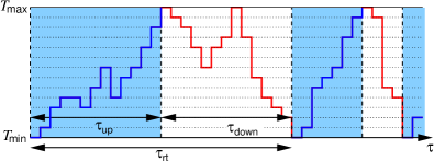
Figure 1: (Color online) Sketch of the random walk that a given replica performs in temperature space in the course of the simulation. Ideally, the replica will wander up ($\tau_{\rm up}$) and down ($\tau_{\rm down}$) in the simulated temperature range $[T_{\rm min},T_{\rm max}]$. The goal of the feedback method is to maximize the number of round trips each replica performs in this temperature range, and thereby minimize the average round-trip time $\tau_{\rm rt}=\tau_{\rm up}+\tau_{\rm down}$.

Our goal is to vary the temperature set $\{T_{i}\}$ of a parallel tempering simulation in such a way that for a given system we speed up equilibration at all temperatures. To accomplish this, we maximize the rate of round trips that each replica performs between the two extremal temperatures $T_{\rm min}=T_{1}$ and $T_{\rm max}=T_{M}$ following a similar approach to the ensemble optimization technique presented in Ref. Trebst et al. (2004). For a given temperature set, we can measure the diffusion of a replica through temperature space by adding a label “up” or “down” to the replica that indicates which of the two extremal temperatures, $T_{\rm min}$ or $T_{\rm max}$ respectively, the replica has visited most recently. The label of a replica changes only when the replica visits the opposite extreme. For instance, the label of a replica with label “up” remains unchanged if the replica returns to the lowest temperature $T_{\rm min}$, but changes to “down” upon its first visit to $T_{\rm max}$. This is illustrated in Fig. 1. For each temperature point in the temperature set $\{T_{i}\}$, we record two histograms $n_{\rm up}(T_{i})$ and $n_{\rm down}(T_{i})$. Before attempting a sequence of swap moves, we increment that histogram at temperature $T_{i}$ which has the label of the respective replica currently at temperature $T_{i}$. If a replica has not yet visited either of the two extremal temperatures, we increment neither of the histograms. This allows us to evaluate for each temperature point the fraction of replicas which have visited one of the two extremal temperatures most recently (e.g., $T_{\rm min}$) as

$$f(T_{i})=\frac{n_{\rm up}(T_{i})}{n_{\rm up}(T_{i})+n_{\rm down}(T_{i})}\;.$$ (3)

The labeled replicas define a steady-state current $j$ from $T_{\rm min}$ to $T_{\rm max}$ that is independent of temperature, e.g., the rate at which “up” walkers are created at $T_{\rm min}$ and – in equilibrium – absorbed at $T_{\rm max}$. In the following we assume that $T$ is a continuous variable, independent of the temperature points in the current temperature set. We can then determine the current $j$ to first order in the derivative as

$$j=D(T)\eta(T)\frac{df}{dT}\;,$$ (4)

where $D(T)$ is the local diffusivity at temperature $T$ and the derivative $df/dT$ is estimated by a linear regression based on the measurements in Eq. (3); $\eta(T)$ is a density distribution indicating the probability for a replica to reside at temperature $T$. We approximate $\eta(T)$ with a step-function $\eta(T)=C/\Delta T$, where $\Delta T=T_{i+1}-T_{i}$ is the length of the temperature interval around temperature $T_{i}<T<T_{i+1}$ for the current temperature set. The normalization constant $C$ is chosen such that

$$\int_{T_{1}}^{T_{M}}\eta(T)dT=C\int_{T_{1}}^{T_{M}}\frac{dT}{\Delta T}=1\;.$$ (5)

Rearranging Eq. (4) gives a simple measure of the local diffusivity $D(T)$ of a replica at temperature $T$

$$D(T)\sim\frac{\Delta T}{df/dT}\;,$$ (6)

where we have dropped the normalization constant $C$ and the current $j$ which is constant for any specific choice of temperature set.

To increase the efficiency of the algorithm, we maximize the current $j$ in temperature space by varying the simulated temperature set $\{T_{i}\}$ and thus varying the probability distribution $\eta(T)$ between the two extremal temperatures, $T_{\rm min}$ and $T_{\rm max}$, which are not changed. In Ref. Trebst et al., 2004 it has been shown that the optimal probability distribution $\eta^{\rm opt}(T)$ is inversely proportional to the square root of the local diffusivity $D(T)$:

$$\eta^{\rm opt}(T)\propto\frac{1}{\sqrt{D(T)}}\;.$$ (7)

For the optimal distribution of temperature points the fraction $f^{\rm opt}(T)$ then decays as

$$\frac{df}{dT}^{\rm opt}=\eta^{\rm opt}(T)\propto\frac{1}{\Delta T^{\rm opt}}\;,$$ (8)

which implies that for any given temperature interval $\Delta T=T_{i+1}-T_{i}$ of the optimal temperature set the fraction has a constant decay

$$\Delta f^{\rm opt}=f^{\rm opt}(T_{i})-f^{\rm opt}(T_{i+1})=1/(M-1)\;,$$ (9)

where $M$ is the number of replicas.

In our algorithm we approach the optimal temperature set and its respective probability distribution by iteratively feeding back measurements of the local diffusivity. After measuring the diffusion of replicas for a given temperature set an improved probability distribution $\eta^{\prime}(T)$ is found as

$$\eta^{\prime}(T)=\frac{C^{\prime}}{\Delta T^{\prime}}=C^{\prime}\sqrt{\frac{1}{\Delta T}\,\frac{df}{dT}}\;,$$ (10)

where the normalization constant $C^{\prime}$ is again chosen so that the normalization condition in Eq. (5) is met. The step-function $\eta^{\prime}(T)$ is still defined for the original temperature set, that is the jumps in the function occur at the temperature points in $\{T_{i}\}$. The optimized temperature set $\{T^{\prime}_{i}\}$ is then found by choosing the $k$-th temperature point $T^{\prime}_{k}$ such that

$$\int_{T^{\prime}_{1}}^{T^{\prime}_{k}}\eta^{\prime}(T)dT=\frac{k}{M}\;,$$ (11)

where $1<k<M$ and the two extremal temperatures $T^{\prime}_{1}=T_{1}$ and $T^{\prime}_{M}=T_{M}$ remain fixed.

We summarize the feedback algorithm by the following sequence of steps

• Start with a trial temperature set $\{T_{i}\}$.

• Repeat

  • Reset the histograms $n_{\rm up}(T)=n_{\rm down}(T)=0$.

  • For the current temperature set perform a parallel tempering simulation with $N_{\rm sw}$ swap moves. After each sequence of swap moves:

    • Update the labels of all replicas.

    • Record histograms $n_{\rm up}(T)$ and $n_{\rm down}(T)$.

  • For the given temperature set estimate an optimized probability distribution $\eta^{\prime}(T)$ via

    $$\eta^{\prime}(T)=C^{\prime}\sqrt{\frac{1}{\Delta T}\,\frac{df}{dT}}\;.$$

  • Obtain the optimized temperatures $\{T^{\prime}_{i}\}$ via

    $$\int_{T_{1}}^{T^{\prime}_{k}}\eta^{\prime}(T)dT=\frac{k}{M}\;.$$

  • Increase the number of swaps $N_{\rm sw}\leftarrow 2N_{\rm sw}$.

• Stop once the temperature set $\{T_{i}\}$ has converged.

The initial number of swaps $N_{\rm sw}$ should be chosen large enough such that a few of round-trips are recorded, thereby ensuring that steady-state data for $n_{\rm up}(T)$ and $n_{\rm down}(T)$ are measured. The derivative $df/dT$ can be determined by a linear regression, where the number of regression points is flexible. Initial batches with the limited statistics of only a few round trips may require a larger number of regression points than subsequent batches with smaller round-trip times and better statistics.

IV Results

IV.1 Ferromagnetic Ising model

In order to illustrate the feedback method, we start with a simple test model, the two-dimensional ferromagnetic Ising model (FM). The Hamiltonian for the model is given by

$${\mathcal{H}}_{\rm FM}=-J\sum_{\langle i,j\rangle}S_{i}S_{j}\;,$$ (12)

where $J=1$ and $S_{i}=\pm 1$ represent Ising spins on a square lattice with $N=L^{2}$ spins. In our simulations we apply periodic boundary conditions and consider nearest-neighbor interactions only. The simple Ising model with uniform couplings has no frustration or disorder, and exhibits a second-order phase transition at $T_{\rm c}=2/\ln(1+\sqrt{2})\approx 2.269$ from a magnetically ordered to a paramagnetic phase.

For simplicity, we define an initial temperature set $\{T_{i}\}$ with $M=21$ temperature points performing a geometric progression, Eq. (2), for a temperature interval $[T_{1}=0.1,T_{M}=10.0]$. The minimum temperature $T_{1}$ is chosen low enough such that the system can approach the zero-temperature ground state of the model, and the maximum temperature $T_{M}$ is chosen well above the critical region of the phase transition. For a short parallel tempering simulation ($N_{\rm sw}=1.6\cdot 10^{7}$, one parallel tempering swap after each lattice sweep) using this initial temperature set, we measure the diffusive current of replicas wandering from the lowest to the highest temperature using an additional label for each replica as described above. In Fig. 2 we show the fraction of replicas diffusing “up” in temperature space. For the geometric temperature set a sharp drop between two temperature points is observed close to the critical region of the phase transition at $T_{c}\approx 2.269$. Similar results are also found for a “flat” temperature set where the acceptance rates are approximately constant around $\sim 40\%$ (with fluctuations of $\sim 10\%$) and independent of temperature, although the drop is not as pronounced.

Calculating the local diffusivity $D(T)$ for the random walk in temperature space using Eq. (6), we find a strong suppression around this critical region as illustrated in Fig. 3. When increasing the size of the simulated system, the dip in the local diffusivity further proliferates, an additional indicator that the slowdown of the random walk in temperature space is dominated by the occurrence of a phase transition. Note the logarithmic scale of the ordinate axis in Fig. 3.

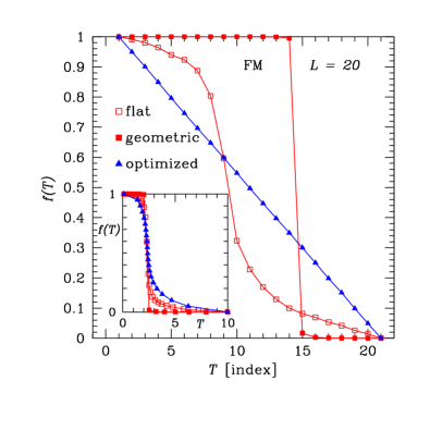
Figure 2: (Color online) Fraction $f(T)$ of replicas diffusing from the lowest to the highest temperature as a function of the temperature index for the ferromagnetic Ising model. For the initial temperature set based on a geometric progression (filled squares), the fraction shows a sharp drop between two temperature points. A similar behavior is found for a temperature set where the acceptance rates are constant $\sim 40\%$ independent of temperature (temperature set with “flat” acceptance rates, open squares). In contrast, for the optimized temperature set (triangles) the fraction constantly decreases. The inset shows the fraction as a function of temperature $T$. The dashed line in the inset represents the critical temperature of the two-dimensional Ising model, $T_{\rm c}\approx 2.269$.

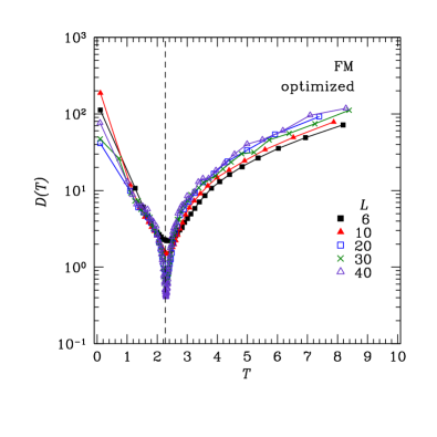
Figure 3: (Color online) Local diffusivity $D(T)$ of the random walk a replica performs in temperature space for the ferromagnetic Ising model as a function of temperature $T$ after the feedback optimization for several system sizes $L$. Notice the logarithmic vertical scale. The vertical dashed line represents $T_{\rm c}\approx 2.269$.

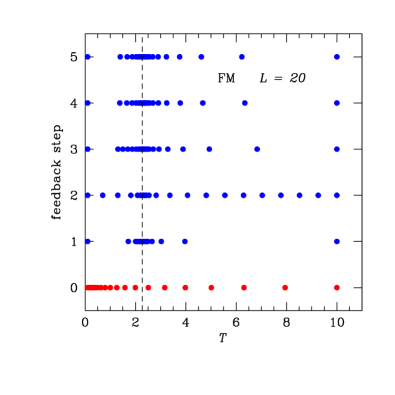
Figure 4: (Color online) Temperature sets for the ferromagnetic Ising model for different feedback steps. Starting from a geometric progression temperature set (step 0), we apply a feedback loop until the temperature set converges. While the geometric progression places many temperatures at low temperatures, the density of temperatures after the feedback optimization is highest at the bottleneck of the simulation around the critical temperature (marked by a vertical dashed line). Rapid convergence of the optimized temperature set is found after 3 – 4 feedback steps and a total of $N_{\rm sw}\approx 1.6\cdot 10^{7}$ swap moves in our parallel tempering simulations.

When applying the feedback, Eq. (11), to define a new temperature set, this suppression in the local diffusivity leads to a concentration of temperature points near the critical temperature as shown in Fig. 4. The feedback thereby tries to compensate for the reduced mobility of replicas in the critical region by reallocating resources towards this temperature range. In contrast, the density of temperatures close to the lowest temperature is greatly reduced, thereby suppressing constant swapping of replicas at low temperatures where for the initial temperature set multiple replicas converged to the fully-polarized ground state configuration.

This effect becomes even more evident when measuring the acceptance probabilities for swap moves as illustrated in Fig. 5. The acceptance probabilities for the initial temperature set based on a geometric progression saturate close to unity for temperatures below $T\lesssim 0.7$, whereas they show a pronounced dip already for small system sizes ($L=20$) around the critical temperature (marked by a vertical dashed line). In contrast, the feedback-optimized temperature set shows a pronounced peak in the acceptance rate $A(T)$ near the critical temperature where temperature points are accumulated by the feedback. Away from the critical temperature region the acceptance probabilities drop. The inset of Fig. 5 shows the acceptance probabilities $A(T)$ for the optimized temperature sets for a fixed number of replicas and varying sizes of the simulated system. While the acceptance probability around the critical temperature remains nearly constant, the exact value away from the critical region decreases with increasing system size. This “mean” acceptance probability away from the bottleneck of the simulation can be tuned by varying the number of simulated replicas.

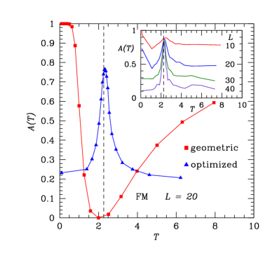
Figure 5: (Color online) Acceptance probabilities $A(T)$ as a function of temperature $T$ for the ferromagnetic Ising model. The inset shows the acceptance rates as a function of temperature in the optimized case for varying system sizes $L$ and a fixed number of temperature points. The vertical dashed line marks the critical temperature.

The fact that for the optimized temperature set the acceptance probabilities vary with temperature contradicts various alternative approaches in the literature Kofke (2004b); Predescu et al. (2004); Kone and Kofke (2005); Rathore et al. (2005); Predescu et al. (2005) that aim at choosing a temperature set in such a way that the acceptance probability of attempted swaps becomes independent of temperature. Naively, one might assume that the choice of constant acceptance rates produces an unbiased random walk in temperature space. This assumption is similar to the idea underlying generalized-ensemble algorithms that aim to sample a flat histogram in the energy such as the multicanonical method Berg and Neuhaus (1991, 1992) or the Wang-Landau algorithm Wang and Landau (2001a, b). For these flat-histogram algorithms, it has been shown that they cannot reproduce the scaling behavior of an unbiased Markovian random walk in energy space, but experience critical slowing down Dayal et al. (2004). This slowdown can be overcome by optimizing the simulated statistical ensemble by a similar feedback algorithm Trebst et al. (2004) as presented here and sampling an optimized histogram that in general is not flat, but reallocates resources towards the bottleneck of the simulation, e.g., in the vicinity of a phase transition or close to the ground state of the system.

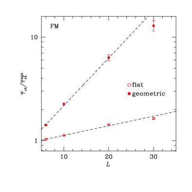
Figure 6: (Color online) Average round-trip times $\overline{\tau}_{\rm rt}$ before the optimization divided by the average round-trip times after the feedback optimization ($\overline{\tau}_{\rm rt}^{\rm opt}$) as a function of system size. The data for the filled squares are for a system starting from a geometric progression and represent the speedup obtained by the feedback method. The open symbols correspond to a temperature set which initially has “flat” acceptance probabilities. The dashed lines are guides to the eye.

Measuring the diffusion of replicas in a subsequent simulation for the optimized temperature set, we find that the current of replicas wandering from the lowest to the highest temperature is now characterized by a constantly decreasing fraction $f(T)$ in agreement with Eq. (9) as shown in Fig. 2 (triangles). In addition, we find that for the optimized temperature set the replicas wander evenly up and down in temperature space, that is $\tau_{\rm up}\approx\tau_{\rm down}$.

In Fig. 6 we show the ratio between the mean round-trip times $\overline{\tau}_{\rm rt}$ before optimization from a geometric and “flat” temperature set divided by the mean round-trip times $\overline{\tau}_{\rm rt}^{\rm opt}$ after optimization in order to illustrate the speedup in replica diffusion attained by the feedback procedure. The data show clearly for all system sizes that the round-trip times after the optimization of the temperature set do not increase as fast as for a geometric progression or “flat” temperature set. Note that for these temperature sets with a fixed number of temperature points the average round-trip times before and after the feedback optimization scale $\sim\exp(aL^{b})$ for the system sizes studied. It is important to note that our algorithm identifies the bottleneck of the parallel tempering simulation that in this model occurs in the form of critical slowing down at the phase transition solely based on measurements of the local diffusivity. The feedback then allows to shift additional resources towards this bottleneck in a quantitative way. In the next section, we apply the algorithm to a more complex model with frustration and a different type of phase transition at zero temperature.

IV.2 Fully-frustrated Ising model

The Hamiltonian of the fully-frustrated (FF) Ising model is given by

$${\mathcal{H}}_{\rm FF}=-\sum_{\langle i,j\rangle}J_{ij}S_{i}S_{j}\;,$$ (13)

where the spins lie on the vertices of a two-dimensional square lattice with periodic boundary conditions. The bonds $J_{ij}$ are chosen such that $|J_{ij}|=1$, but with the constraint that the product of the bonds around all plaquettes of the system is negative, i.e.,

$$\prod_{\Box}J_{ij}=-1\;.$$ (14)

The model does not order at finite temperatures, but exhibits a critical point at zero temperature. In the vicinity of this transition to a highly degenerate ground-state manifold, the system relaxes very slowly.

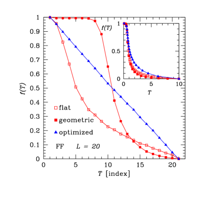
Figure 7: (Color online) Fraction $f(T)$ of replicas diffusing from the lowest to the highest temperature for the fully frustrated Ising model. Displayed are data for an initial “flat” temperature set with $M=21$ temperature points that yields temperature-independent acceptance probabilities for swap moves (open squares). In addition, data for a geometric progression ($M=21$) are also shown (filled squares). After the optimization, the change in the fraction is independent of the temperature index (triangles). The inset shows the fractions as a function of temperature $T$. Data for $N_{\rm sw}=2\cdot 10^{6}$.

In this section, we discuss our feedback optimization algorithm for two choices of the initial temperature set. First we start from the temperature set introduced in Sec. IV.1 computed with a geometric progression, Eq. (2), which has $T_{\rm min}=0.1$, $T_{\rm max}=10.0$ and $M=21$ temperatures. In this first approach, we keep the number of temperature points constant for all system sizes $L$. In the second approach, we choose an initial temperature set where we fix again $T_{\rm min}$ and $T_{\rm max}$ to the aforementioned values but tune the number of temperatures $M$ as well as their position in such a way that we obtain acceptance probabilities for swap moves that are approximately independent of the temperature (“flat”) with a mean value of $A(T)\sim 40\%$ and deviations around this mean value of maximally 10% ffi .

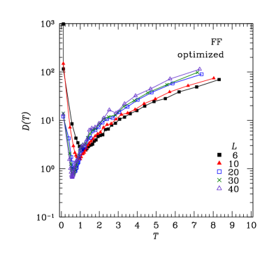
Figure 8: (Color online) Local diffusivity $D(T)$ of a random walk in temperature space for the fully-frustrated Ising model as a function of temperature $T$ after the feedback optimization for several system sizes $L$. Notice the logarithmic vertical scale.

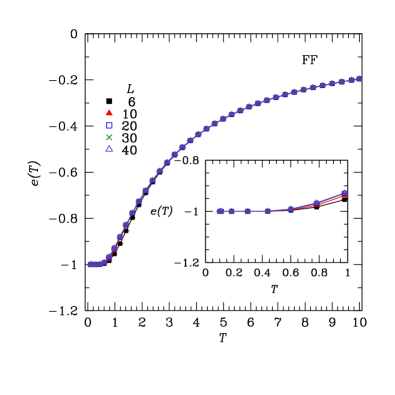
Figure 9: (Color online) Energy per spin $e(T)=(1/N)[\langle{\mathcal{H}}\rangle]_{\rm av}$ as a function of temperature $T$ for the fully-frustrated Ising model for several system sizes. The data show that already for $T\lesssim 0.5$ the energy is independent of temperature, thus signaling that the system has reached the ground state. The inset zooms into the temperature range around $T=0$.

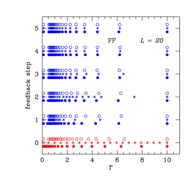
Figure 10: (Color online) Temperature sets for the fully-frustrated Ising model for different feedback steps. Starting from a temperature set where the acceptance probabilities are independent of temperature with $M=21$ temperature points (open symbols) and a temperature set obtained by a geometric progression also with $M=21$ temperature points (filled symbols), we apply repeated feedback steps until the temperature sets converge to the optimal distributions. Also shown are data for an initial temperature set with $M=21$ equidistant temperature points (stars). Independent of the initial temperature set, an optimal temperature distribution is found after 3 – 4 iterations and $\sim 7.5\cdot 10^{6}$ swaps. After the successful feedback, temperature points accumulate near the transition to the ground state slightly above zero temperature.

We show the fraction $f(T)$ of replicas diffusing from the lowest to the highest temperature as a function of the temperature index in Fig. 7. Similar to the Ising model, the data for the geometric progression temperature set deviate considerably from a straight line which is expected for the optimal temperature distribution. A similar behavior is found when starting from a temperature set that initially has temperature-independent acceptance probabilities. The local diffusivity in temperature space calculated from the measured diffusive current is plotted in Fig. 8. There is a pronounced dip in the diffusivity around $T\approx 0.5$ that we can identify as the temperature region where the system enters the highly degenerate ground-state manifold, e.g., by calculating the energy of the system, as plotted in Fig. 9. Again we find that the diffusivity points to a strong bottleneck of the simulation at the critical point which for the fully frustrated Ising model is at the transition to the zero-temperature ground-state manifold. The general shape of the diffusivity in the vicinity of this bottleneck remains unchanged with respect to the feedback. By applying the feedback method, additional temperature points are shifted towards this bottleneck which is illustrated in Fig. 10 for the geometric progression (full symbols) as well as the “flat” temperature set (open symbols). For moderately large system sizes, we again find rapid convergence of the generated temperature sets within 3 – 4 feedback steps and a total of $N_{\rm sw}\approx 7.5\cdot 10^{6}$ swap moves. For the optimized temperature set, the diffusive current is again characterized by a fraction of replicas drifting from the lowest to the highest temperature that linearly decreases with the temperature index, see Fig. 7 (triangles).

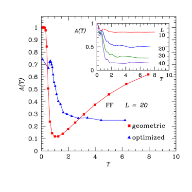
Figure 11: (Color online) Acceptance probabilities $A(T)$ for replica swap moves as a function of temperature $T$ for the fully-frustrated Ising model. While the acceptance probabilities for a geometric progression temperature set show a pronounced dip close to $T=0$, the optimized ensemble shows a peak close to zero temperature where the system enters the ground-state manifold. The inset shows, for a fixed number of temperatures, the acceptance rates as a function of temperature for different system sizes $L$. As for the Ising model, the “mean” value away from the bottlenecks can be tuned by increasing the number of temperatures. This illustrates that in order to obtain higher acceptance rates away from the bottlenecks of the simulation, the number of temperatures have to be increased with increasing $L$.

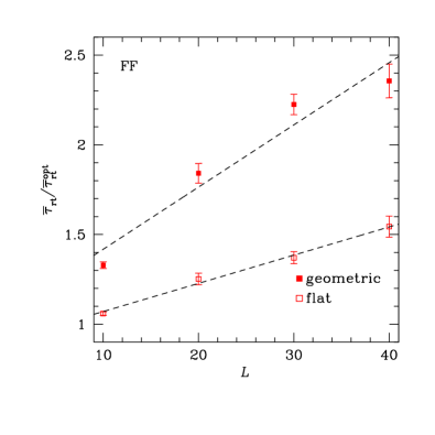
Figure 12: (Color online) Average round-trip times $\overline{\tau}_{\rm rt}$ before the optimization divided by the average round-trip times after the feedback optimization ($\overline{\tau}_{\rm rt}^{\rm opt}$) as a function of system size for the fully-frustrated Ising model. The data for the filled squares are for a system starting from a geometric progression temperature set and represent the speedup obtained by the feedback method. In addition, we show data for a temperature set with “flat” temperature-independent acceptance rates (open squares). The dashed lines are guides to the eye.

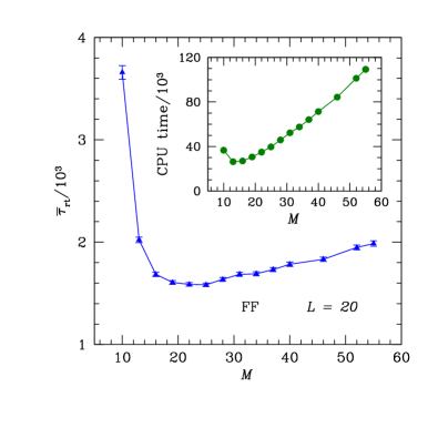
Figure 13: (Color online) Average round-trip times $\overline{\tau}_{\rm rt}$ as a function of the number of temperatures $M$ for the fully-frustrated Ising model with $L=20$ after the feedback optimization. The data show that the round-trip times only depend moderately on the number of temperatures $M$, provided that there is sufficient overlap of the energy distributions. For a small number of replicas, this is no longer the case and the round-trip times increase drastically, e.g., for $M\lesssim 12$ in this plot. The inset shows the CPU time which is the product of the average round-trip time with the number of temperatures $M$. The data show a more pronounced minimum.

The acceptance probabilities $A(T)$ for replica swap moves are shown in Fig. 11 for simulations with a geometric progression and the optimized temperature set. While the acceptance probabilities peak at unity close to zero and dramatically drop in the geometric progression temperature set, in the optimized set most temperatures are reshuffled to the low-temperature region slightly above zero temperature where the system enters the highly degenerate ground-state manifold. The inset to Fig. 11 shows the acceptance probabilities as a function of temperature for a fixed number of temperatures, as well as $T_{\rm min}=0.1$ and $T_{\rm max}=10.0$ fixed. As in the case for the ferromagnet, the “mean” acceptance probability away from the ground state bottleneck seems almost independent of temperature and settles at a value that is determined by the number of temperatures used for a given system size $L$.

In order to test the efficiency of the feedback method on the FFIM, in Fig. 12 we show the ratio between the mean round-trip times $\overline{\tau}_{\rm rt}$ before optimization divided by the mean round-trip times $\overline{\tau}_{\rm rt}^{\rm opt}$ after optimization in order to illustrate the speedup in replica diffusion attained by the feedback procedure. The data show clearly for all system sizes that the round-trip times after the optimization of the temperature set do not increase as fast as for a geometric progression or “flat” temperature set. For these temperature sets where the number of temperature points increases with system size we find that the average round-trip times scale $\sim a+bx^{c}$.

Finally, we discuss the effects of varying the number of temperatures $M$ in the temperature set. Figure 13 shows the average round-trip times for the fully frustrated Ising model ($L=20$) as a function of the number of temperatures $M$. For $M\gtrsim 12$, the average round-trip times show only moderate variations with the number of temperature points $M$, whereas for a smaller number of temperatures the average round-trip times increase drastically. This can be understood by keeping in mind that a parallel tempering swap will only be accepted with a high probability if the energy distributions between neighboring temperatures overlap. If the minimum and maximum temperatures are fixed and $M$ is reduced, the energy distributions will cease to overlap, which accounts for the increased average round-trip times. Factoring in the total CPU time, which we define as the product of the average round-trip time with the number of temperatures, the minimum is more pronounced (inset to Fig. 13) and clearly illustrates that while a larger number of temperatures has little effect on the round-trip times, the total CPU time increases drastically with increasing $M$.

Because the data for the average round-trip times vs $M$ have an optimal value, it is conceivable to develop a feedback optimization method that optimizes both the position of the temperatures and the number of temperatures $M$. Furthermore, in addition to optimizing the number and locations of the temperature points, we have also explored varying the ratio of the number of sweep moves attempted to the number of replica-swap moves attempted, since this is yet another parameter one must set in a parallel tempering simulation. This ratio can be adjusted globally (the same ratio at all temperatures) or locally (the ratio optimized independently at each temperature). This will be discussed in more detail in a subsequent communication.

IV.3 Spin glasses

Since the optimization of temperature sets improves the sampling for the two paradigmatic spin models discussed above, it is a natural step to ask how this feedback optimization technique can be applied to improve state-of-the-art parallel tempering simulations of Ising spin glass models, such as the three-dimensional (3D) Edwards-Anderson Ising spin glass Edwards and Anderson (1975); Binder and Young (1986):

$${\mathcal{H}}_{\rm SG}=-\sum_{\langle i,j\rangle}J_{ij}S_{i}S_{j}.$$ (15)

Here the spins lie on the vertices of a cubic lattice with periodic boundary conditions. The bonds $J_{ij}$ are chosen according to a Gaussian distribution with zero mean and standard deviation unity. The system undergoes a spin-glass transition at $T_{\rm c}=0.951(9)$ Bhatt and Young (1988); Marinari et al. (1998); Katzgraber et al. (2006).

For the spin glass there is the additional complexity that different disorder realizations can lead to strong sample-to-sample variations. Thus one could also surmise that strong sample-to-sample variations exist for the time it takes to equilibrate individual samples. This becomes evident when measuring the round-trip times for replicas in a standard parallel tempering simulation with a fixed temperature set, as illustrated in Fig. 14 for the Edwards-Anderson Ising spin glass. We find that the measured round-trip times follow a fat-tailed Fréchet distribution Gumbel (1958); tai (solid line, fit performed with R R ). The integrated generalized extreme value distribution is given by:

$$H_{\xi;\mu;\beta}(\tau)=\exp\left[-\left(1+\xi\frac{\tau-\mu}{\beta}\right)^{1/\xi}\right]\;.$$ (16)

Here $\mu$ represents a generalized most probable value (location parameter) and $\beta$ a standard deviation (scale parameter). The value of the shape parameter $\xi$ determines whether the distribution is thin-tailed ($\xi<0$, Weibull), Gumbel ($\xi=0$), or fat-tailed ($\xi>0$, Fréchet) Gumbel (1958). Note that when $\xi>0$, the $m$-th moment of the Fréchet distribution exists only if $|\xi|<1/m$, e.g., if $\xi>1/2$ the variance of the distribution is not properly defined. Our results are in agreement to similar observations for broad-histogram simulations Dayal et al. (2004); Alder et al. (2004); Costa et al. (2005). Note that the distribution is increasingly more fat-tailed as the system size increases (see the inset to Fig. 14).

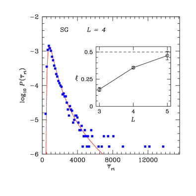
Figure 14: (Color online) Distribution of average round-trip times for 5000 different samples of the 3D Edwards-Anderson Ising spin glass with Gaussian disorder and fixed system size $L=4$ in the temperature range from $T_{\rm min}=0.10$ to $T_{\rm max}=2.0$. The data follow a fat-tailed Fréchet distribution (solid line) with a shape parameter $\xi=035(1)$. The inset shows the shape parameter $\xi$ as a function of system size $L$. Already for $L\gtrsim 5$, the shape parameter becomes $\xi\gtrsim 1/2$, indicating that the variance of the distribution is no longer properly defined. The simulations have been performed using a fixed temperature set with $M=27$ temperature points distributed such that, on average, replica swap moves have a nearly flat acceptance rate.

The measurement of the round-trip times thus allows to classify individual spin-glass samples as “typical” with round-trip times in the bulk of the distribution or “hard” with round-trip times in the tail of the distribution. Such a classification can be very useful to shift computational resources towards the “hard” samples in the course of a simulation as these samples potentially might require substantially longer simulation times in order to equilibrate. Preliminary tests suggest correlations between round-trip and equilibration times. The observation of strong sample-to-sample variations in the distribution of round-trip times also raises the general question, whether previous spin-glass studies have properly equilibrated the “hardest” samples in their simulations. It remains to be verified whether this introduces a systematic error in the analysis of spin-glass systems. Specifically, the finite-size scaling should be sensitive to such systematic errors, as it has been observed that the number of “hard” samples significantly increases with system size, see the inset in Fig. 14 and Refs. Dayal et al., 2004, Alder et al., 2004, and Costa et al., 2005.

On the other hand, we can ask whether we can optimize the simulated temperature set and generate a “common” temperature set for samples from the various parts of the distribution. To do so, we apply the feedback optimization outlined above in such a way that we generate a common probability distribution ${\bar{\eta}}(T)$ for a set of samples that are each characterized by their own diffusivity $D_{i}(T)$, steady-state fraction $f_{i}(T)$ and current $j_{i}$, which are related by

$$j_{i}=D_{i}(T){\bar{\eta}}(T)\frac{df_{i}}{dT},$$ (17)

where the index $i$ indicates the samples in the given set. Rearranging this equation, the local diffusivity of an individual sample can be expressed as

$$D_{i}(T)=\frac{j_{i}}{{\bar{\eta}}(T)\cdot df_{i}/dT}\;.$$ (18)

To ensure equilibration of all samples we want to simulate each sample for a fixed number of round trips, despite the strong sample-to-sample variations. In order to minimize the overall computer time spent to simulate such a set of samples, we then minimize the sum of round-trip times $\sum_{i}\tau_{i}$. This is equivalent to minimizing the sum of the inverse of all currents, i.e., $j_{i}^{-1}$, since the current $j_{i}$ is inversely proportional to the round-trip time $\tau_{i}$. Following a similar line of arguments as for the original temperature set optimization, we find that the optimal common temperature distribution ${\bar{\eta}}^{\rm opt}(T)$ is proportional to the square root of the sum of inverse local diffusivities

$${\bar{\eta}}^{\rm opt}(T)\propto\sqrt{\sum_{i}\frac{1}{D_{i}(T)}}\;.$$ (19)

Again we can use a feedback loop to find an optimized common temperature set by feeding back the measured local diffusivities

$${\bar{\eta}}^{\rm opt}(T)=C\sqrt{{\bar{\eta}}(T)\sum_{i}\left(\tau_{i}\cdot\frac{df_{i}}{dT}\right)}\;,$$ (20)

where $C$ is a normalization constant. The common optimized temperature set is then found using a partial integration as given in Eq. (11).

V Conclusions

We have introduced an approach to systematically optimize temperature sets for parallel tempering Monte Carlo simulations using an adaptive feedback method that is motivated by a recently developed ensemble optimization technique for broad-histogram Monte Carlo simulations Trebst et al. (2004). We have applied the method to two paradigmatic spin models, the ferromagnetic Ising model and the fully frustrated Ising model in two dimensions. For both models we have shown that the feedback technique improves sampling of the phase space by reducing the average round-trip time of replicas diffusing in temperature space.

Probably our most important result is the insight, that the common wisdom that temperature sets in parallel tempering Monte Carlo should yield temperature-independent acceptance probabilities for the swap moves is not necessarily an optimal choice. Our feedback algorithm shifts temperature points in the optimized temperature sets towards the bottlenecks of the simulation, typically in the vicinity of a phase transition, where equilibration is suppressed. In particular, this has the effect that the acceptance probabilities for replica swap moves are higher around the bottlenecks and are not temperature independent for the so-optimized temperature sets.

We also outline an approach to define “common” temperature sets for systems that require configurational averages, such as spin glasses. In addition, we have briefly discussed the effects of sample-to-sample fluctuations with respect to equilibration times of individual spin glass samples, thus pointing towards a potential source of systematic errors in previous numerical studies of spin glasses.

Clearly a deeper analysis of feedback-optimized parallel tempering Monte Carlo is needed, in particular in the context of spin glasses, as well as the questions raised at the end of Sec. IV.2.