Strong Griffiths singularities in random systems and their relation to extreme value statistics

Abstract

We consider interacting many particle systems with quenched disorder having strong Griffiths singularities, which are characterized by the dynamical exponent, $z$, such as random quantum systems and exclusion processes. In several $d=1$ and $d=2$ dimensional problems we have calculated the inverse time-scales, $\tau^{-1}$, in finite samples of linear size, $L$, either exactly or numerically. In all cases, having a discrete symmetry, the distribution function, $P(\tau^{-1},L)$, is found to depend on the variable, $u=\tau^{-1}L^{z/d}$, and to be universal given by the limit distribution of extremes of independent and identically distributed random numbers. This finding is explained in the framework of a strong disorder renormalization group approach when, after fast degrees of freedom are decimated out the system is transformed into a set of non-interacting localized excitations. The Fréchet distribution of $P(\tau^{-1},L)$ is expected to hold for all random systems having a strong disorder fixed point, in which the Griffiths singularities are dominated by disorder fluctuations.

I Introduction

In interacting many-particle systems quenched (i.e. time independent) disorder can induce unusual physical properties which do not exist in non-random systems. For example in a random ferromagnet the linear susceptibility, $\chi$, is divergent in an extended part of the paramagnetic phase, which is called Griffiths phasegriffiths . This type of singular behavior is caused by rare regions of the sample, in which due to strong disorder fluctuations the local couplings are much stronger than their average and they are even stronger than the disordering field, such as the temperature in a classical system. Consequently these rare regions are locally in the ferromagnetic phase and the relaxation process associated to them involves a very large relaxation time, $\tau$. In the thermodynamic limit the distribution of the $\tau$-s has no upper limit which leads to singularities in several average physical quantities. One can say that these Griffiths singularities are controlled by a line of semi-critical fixed points, having a diverging relaxation time but a finite correlation length, $\xi$. In a classical disordered system in which the phase transition is triggered by the variation of the temperature these singularities are very weakharris and often one needs astronomical times to be able to observe them. There are, however, another type of random systems in which the Griffiths effects are much stronger and one can measure them in conventional experiments.

Strong Griffiths effects can be observed, among others, in random quantum systemsqsg at zero temperature, $T=0$, in which a quantum phase transition can take place by varying a control parameter, $\delta$. The prototype of random quantum systems is the random transverse-field Ising model (RTIM), which is defined in one dimension (1d) by the Hamiltonian,

$$H=-\sum_{i=1}^{L-1}\lambda_{i}\sigma_{i}^{x}\sigma_{i+1}^{x}-\sum_{i=1}^{L}h_{i}\sigma_{i}^{z}\;,$$ (1)

in terms of the Pauli matrices, $\sigma_{i}^{x,z}$, at site $i$. The exchange couplings, $\lambda_{i}$, and the transverse fields, $h_{i}$, are both independent and identically distributed (iid) random variables and the control parameter is definedfisher as:

$$\delta=\frac{[\ln h]_{\rm av}-[\ln\lambda]_{\rm av}}{{\rm var}[\ln\lambda]+{\rm var}[\ln h]}\;.$$ (2)

Here and in the following we use $[\dots]_{\rm av}$ to denote averaging over quenched disorder and ${\rm var}[x]$ stands for the variance of $x$. The system is in the ferromagnetic (paramagnetic) phase for $\delta<0$ ($\delta>0$) and the quantum critical point is located at $\delta=0$. It was first McCoymccoy who calculated exactly the average susceptibility of this model and found that $[\chi]_{\rm av}$ is divergent in a finite regime of the paramagnetic phase. Later the excitation energy, $\epsilon\sim 1/\tau$, is shownfisher to vanish with the size of the system as:

$$\epsilon\sim L^{-z}\;,$$ (3)

with the dynamical exponent, $z>0$, which is a continuous function of $\delta$.

Another class of problems with strong Griffiths effects are stochastic many-particle systemsschutzreview ) with quenched disorderkrug , such as the 1d partially asymmetric simple exclusion process (PASEP)) with position or particle dependent hopping ratesASEP ; pasep_sw or the zero range process (ZRP) with disorderZRP . Also reaction-diffusion modelshinrichsen with quenched disorder might show strong Griffiths effectscontact , see, howevervojta ; odor . As an example we consider here the PASEP with particle-wise (pw) disorderASEP , in which the $i$-the particle, $i=1,2,\dots,N$, can hop to empty neighboring sites with a rate $p_{i}$ to the right and $q_{i}$ to the left in a 1d periodic lattice with $L>N$ sites. Here the hop rates are iid random numbers and the control parameter is defined as:

$$\delta_{p}=\frac{[\ln p]_{\rm av}-[\ln q]_{\rm av}}{{\rm var}[\ln p]+{\rm var}[\ln q]}\;,$$ (4)

so that the particles move to the right (to the left) for $\delta_{p}>0$ ($\delta_{p}<0$). Here we restrict ourselves to the domain, $\delta_{p}\geq 0$. Strong Griffiths effects in the PASEP are caused by such rare particle clusters in which the local hopping rates of the particles prefer jumps against the global bias. As a result in the anomalous diffusion regime, which can be called as the Griffiths phase of the PASEP, the average displacement of particles grows in time as

$$\langle x(t)\rangle\sim t^{1/(1+z_{p})},$$ (5)

when the system undergoes a coarsening process. Here, the dynamical exponent of the PASEP, $z_{p}>0$, is a continuous function of $\delta_{p}$. Note that outside the Griffiths phase, $\delta>\delta_{G}$, the stationary velocity of the particles is $v=O(1)$, whereas in the Griffiths phase it vanishes asASEP :

$$v\sim L^{-z_{p}}\;.$$ (6)

In general Griffiths singularities are characterized by the distribution of the relaxation times of slow processes or equivalently by the distribution of their inverse, $1/\tau$, which is just the excitation energy, $\epsilon$, of the RTIM and the stationary velocity, $v$, of the PASEP. In a finite system $1/\tau$ is just the smallest event associated to one of the rare regions and the occurrence of these rare regions as well as the distribution of $1/\tau$ depends on the form of the randomness in the dynamical model. In the mathematical literature such questions are studied in the frame of extreme value statisticsgalambos (EVS) and rigorous results are known for iid random variables, which are distributed according to a parent distribution, $\pi(y)$ ($y=1/\tau$). In this case the limit distributions are in a few different universal scaling forms depending on the asymptotic behavior of the parent distribution for large values of $y$. If the decay of $\pi(y)$ is faster than any power then it is the Gumbel distribution, for power-law tails it is the Fréchet distribution and for power-laws with an edge the Weibull distribution is the result. If the random variables are not iid there are no general mathematical results, however a few special cases have been studied and solvedgalambos . Among others we can mention the statistics of extreme intensities of Gaussian interfacesracz which generally does not coincide with the known limit distributions of iid variables. Similarly, for hierarchically correlated variables the limit distribution deviates from the Gumbel formdean .

As we described above strong Griffiths affects are present in interacting particle systems having strong temporal and spatial correlations, therefore at first thought it seems unlikely that a simple connection with the theory of EVS exists. A closer look, however, shows that in a class of systems the rare events, which are the source of Griffiths singularities, are well localized and separated in such a way that they could be considered independent. For these systems then the distribution function, $P_{L}(1/\tau)$, could correspond to the appropriate limit distribution of EVS.

In this paper we are going to study this issue in more details. For some random 1d models having a small correlation length we perform exact calculations. On the other hand at a general point of the Griffiths phase a renormalization group (RG) approachim is applied, which is expected to give asymptotically exact dynamical singularities in the Griffiths phase. The RG equations can be analytically solved for some 1d random models, such as for the RFIMfisher and for the PASEPASEP , in other cases and in higher dimensions one resort to numerical calculations. For some 1d random models we also calculate numerically the different distribution functions.

The structure of the paper is the following. In Sec.II we consider Griffiths singularities in random quantum systems. In more details we study the 1d RTIM, but also the random quantum Potts chain, as well as the RTIM for ladders and in 2d and the random Heisenberg model in 1d and 2d are investigated. In Sec.III we study Griffiths singularities in random stochastic systems, such as in the PASEP with particle-wise and site-wise disorder. Our paper is closed by a discussion in Sec.IV.

II Griffiths singularities in random quantum systems

II.1 The RTIM in 1d

II.1.1 Exact results for extreme disorder

In order to gain some insight into the origin of Griffiths singularities we solve exactly the RTIM in Eq.(1) using the bimodal distribution: $\lambda_{i}=\lambda$, with probability $c$ and $\lambda_{i}=\lambda^{-1}$ with probability $1-c$, and $h_{i}=1$. Furthermore we take the limit $c\ll 1$, when most of the couplings are weak and $\lambda\gg 1$, so that we are deeply in the paramagnetic phase. There are, however, rare regions in which all the couplings, say $n$, are strong and appear with an exponentially small density, $\rho(n)=c^{n}$. Such a cluster is typically embedded into a see of very weak couplings, thus the corresponding excitation energy is obtained by solving the gap in a cluster with free boundary conditions, leading to: $\epsilon(n)\approx\lambda^{-n}$. Now we obtain that the distribution of the excitation energies in an infinite system has a power-law tail:

$$P(\epsilon)\approx\frac{1}{\ln\lambda}\epsilon^{\omega},\quad\epsilon\to 0\;,$$ (7)

and the gap exponent, $\omega$, is given by:

$$\omega=\frac{\ln(1/c)}{\ln\lambda}-1\;.$$ (8)

In a finite system of size, $L$, the typical size of the largest cluster, $n_{1}$, is given by the condition, $L\sum_{n\geq n_{1}}\rho(n)=1$, so that the typical value of the smallest gap, $\epsilon_{1}$, is given by: $\epsilon_{1}=L^{-z}$, with the dynamical exponent defined in Eq.(3):

$$z=\frac{\ln\lambda}{\ln(1/c)}\;.$$ (9)

Note that we obtain the relation, $\omega=1/z-1$, so that the distribution function for finite systems satisfies the scaling formyr96 :

$$P_{L}(\epsilon_{1})=L^{z}\tilde{P}_{1}(\epsilon_{1}L^{z})\;,$$ (10)

and the subscript of the scaling function, $\tilde{P}_{1}(u)$, refers to the first gap. In the following we determine the scaling function. First, we note that the rare regions in the system are localized thus they could be placed at $\sim L$ different positions of the chain. Furthermore the different rare regions are independent and their lengths, which are proportional to the log-gap, is distributed by the same exponential distribution. From these follows that $\epsilon_{1}$ is the smallest gap out of $\sim L$ independent possible gaps, associated to the different rare regions, and the gaps are distributed by the same parent distribution given in a power-law form in Eq.(7). Consequently in the large-$L$ limit the distribution function, $\tilde{P}_{1}(u)$, is given by the standard Fréchet distributiongalambos :

$$\tilde{P}_{1}(u)=\frac{1}{z}u^{1/z-1}\exp(-u^{1/z})\;,$$ (11)

and $u=u_{0}\epsilon_{1}L^{z}$, where the non-universal constant, $u_{0}$, depends on the amplitude of the tail in Eq.(7).

II.1.2 Analytical results of the strong disorder RG

The strong disorder RG methodim has been introduced by Ma and Dasguptamdh to study random antiferromagnetic Heisenberg chains. For the 1d RTIM Fisherfisher has applied the method and solved analytically the RG equations in the vicinity of the random quantum critical point. During renormalization the strongest local term in the Hamiltonian, coupling or transverse field, is decimated out and between remaining sites new interactions are generated through perturbation calculation. If a strong bond, say $\lambda_{2}$, connecting sites $1$ and $2$ is decimated out the effective transverse field, $\tilde{h}$, acting on the two-site cluster is given byfisher :

$$\tilde{h}=\frac{h_{1}h_{2}}{\kappa\lambda_{2}}\;,$$ (12)

where $\kappa=1$. On the contrary if a strong transverse field, say $h_{2}$ and thus the site $2$ is decimated out the effective coupling, $\tilde{\lambda}$, connecting the remaining sites, $1$ and $3$ is given byfisher :

$$\tilde{\lambda}=\frac{\lambda_{1}\lambda_{2}}{\kappa h_{2}}\;,$$ (13)

with $\kappa=1$. As renormalization goes on the energy scale, set by the strength of the strongest local term in the Hamiltonian, gradually decreases and the distributions of the renormalized couplings and transverse fields approach their fixed-point form. At the critical point couplings and transverse fields are decimated symmetrically and their fixed-points distribution functions are identical and have the so called infinite disorder propertyfisher : the ratio of any two terms tends either to zero or to infinity. Consequently the decimation rules become exact and the critical singularities, both static and dynamical ones are asymptotically exact. In the disordered Griffiths phase, which is a part of the paramagnetic phase after a starting period of the RG when spin clusters of typical size, $\xi$, are formed almost exclusively transverse fields are decimated out. At the fixed point the energy scale still goes to zero and the decimation equations are asymptotically exact leading to exact dynamical singularities, however the spatial correlations are short-ranged and correct only up to a range of $\xi$. The analytical solution of the RG equations by Fisherfisher is exact up to $O(\delta)$ which is then extended into the complete Griffiths phaseijl ; i02 . The dynamical exponent, $z$, is found to be the positive root of the equationi02 :

$$\left[\left(\frac{\lambda}{h}\right)^{1/z}\right]_{\rm av}=1\;,$$ (14)

which has also been derived by a mapping with the random random walkir98 . For the binary disorder used in the previous section this leads to: $\lambda^{1/z}c+\lambda^{-1/z}(1-c)=1$, having the solution in Eq.(9) in the limit $c\ll 1$. Note that this result is valid for any value of $\lambda>1$, which is connected to the fact that the gap of a large $n$-bond cluster in a see of weaker bonds scales as: $\epsilon(n)\sim\lambda^{-n}$. The dynamical exponent in Eq.(14) is a continuous function of $\delta$, and in the vicinity of the critical point it is divergent asfisher $z\approx 1/2\delta$. It can be shown by the RG calculation that the low temperature behavior of the average susceptibility and that of the specific heat, $c_{V}$, are given byfisher ; i02 :

$$\chi(T)\sim T^{-1+1/z},\quad c_{V}(T)\sim T^{1/z}\;,$$ (15)

thus the singularity involves the dynamical exponent. Note that at zero temperature $\chi(0)$ is divergent for $z>1$.

The distribution of the smallest energy gap in a finite chain of length, $L\gg\xi$, and in the vicinity of the critical point: $0<\delta\ll 1$ is calculated by Fisher and Youngfisheryoung . For the distribution of the log-gap, $G=-\ln\epsilon_{1}$, they obtained:

$$d{\rm Prob}[G|L]\approx 2\delta Ln_{G}\exp(-Ln_{G})dG\;,$$ (16)

where

$$n_{G}\approx 4\delta^{2}\exp(-2\delta G)\;$$ (17)

is the density of remaining clusters. Here making use of the fact that in the vicinity of the critical point the correlation length is given byfisher $\xi\sim\delta^{-2}$ and $z\approx 1/2\delta$ we obtain:

$$n_{G}\sim\frac{\epsilon_{1}^{1/z}}{\xi}\;.$$ (18)

Inserting Eq.(18) into Eq.(16) we obtain that the scaling variable is $u=u_{0}\epsilon_{1}(L/\xi)^{z}$, in terms of which the distribution is in the Fréchet form in Eq.(11).

II.1.3 Phenomenological considerations

Results of the previous two subsections indicate that the distribution of the smallest gap of the RTIM in 1d is the Fréchet distribution, at least in the limiting cases i) extreme binary disorder with $\xi\ll 1$ but $z$ is arbitrary (Sec.II.1.1) ii) arbitrary form of disorder, but $\delta\ll 1$ (Sec.II.1.2). Here we argue that the Fréchet form of the distribution should be generally valid in the disordered Griffiths phase, at least if the low-energy excitations in the system are localized. Here we note that performing the RG up to an energy scale, $\Omega_{0}$, which is much smaller than $\Omega_{\xi}\sim\xi^{-z}$, we obtain an equivalent random spin chain with very weakly interacting effective spins. Typically, the log-bonds are in the order of $-\ln\tilde{\lambda}\sim\Omega_{0}^{-1/z}$, so they are small compared to the value of effective fields $\tilde{h}\Omega_{0}$i02 . Consequently, in the following RG steps almost exclusively transverse-fields are decimated out through the transformation in Eq.(13), which does not influence the transverse fields of the other active spins. At the energy scale, $\Omega_{0}$, the effective transverse fields, $\tilde{h}$, have a power-law distribution $P(\tilde{h})\sim\tilde{h}^{-1+1/z}$, and the smallest one gives thus the smallest gap of the chain. Consequently the renormalized chain satisfies the conditions needed for the validity of the Fréchet limit distribution. Generally, for the $n$-th excitation energy the limit distribution is given bygalambos :

$$\tilde{P}_{n}(u_{n})=\frac{1}{z}u_{n}^{n/z-1}\exp(-u_{n}^{1/z})\;,$$ (19)

in terms of $u_{n}=u_{0}L^{z}\epsilon_{n}$. We note that the gap exponent is now, $\omega_{n}=n/z-1$, which has been obtained beforeijr through scaling considerations.

This type of reasoning for the smallest gap applies to another random systems, too, provided the decimation rules are analogous to those in Eqs.(12) and (13). In d-dimensions the only difference is that $z$ is replaced by $z/d$, provided the strong disorder RG approach leads to localized, non-interacting effective degrees of freedom.

Next, the distribution of excitation energies is analyzed in the ordered phase of the RTIM. In $1d$ due to duality the disordered and ordered phases are related to each other and in the RG procedure the role of the couplings and the transverse-fields are exchanged. Consequently, at the energy-scale, $\Omega_{0}\ll\Omega_{\xi}$, the typical log-fields are $-\ln\tilde{h}\sim\Omega_{0}^{-1/z}$, whereas $\tilde{\lambda}\sim\Omega$. Thus the renormalized chain is a classical random bond Ising chain with very small effective transverse fields having an exponentially vanishing first gap. The dynamical properties of the chain are governed by kink-like excitationshuse . In an open chain the lowest excitation is one kink, which corresponds through duality to a spin flip in the disordered phase. Consequently the distribution of the second gap in an open chain follows the Fréchet distribution. On the contrary for a closed chain the lowest excitation involves two kinks and the corresponding excitation energy is the sum of the first two smallest effective couplings of the renormalized chain. Consequently the distribution of the second gap in a closed chain is related to the solution of the above extreme value problem. In higher dimensions the singularities in the ordered Griffiths phase have a more complicated structuremotrunich . Here the renormalized system is a random bond Ising model with a complicated topology, and the (second) excitation, which is relevant in the dynamical properties corresponds to the creation of an oppositely magnetized domain. The excitation energy is just the sum of the effective couplings at the boundary of the domain.

In the following we check the above conjectures by numerical calculations.

II.1.4 Distribution of gaps from numerical diagonalization

The RTIM in 1d can be transformed into a problem of free fermions and the calculation of the gaps necessities the diagonalization of a $2L\times 2L$ tridiagonal matrix the entries of which are the couplings and the transverse fieldsbigpaper . In the numerical calculation we used a continuous, uniform distribution: $\pi_{\lambda}(\lambda)=1$ for $0<\lambda\leq 1$ and $0$ otherwise; as well as $\pi_{h}(h)=1/h_{0}$, for $0<h\leq h_{0}$ and $0$ otherwise. The critical point is located at $h_{0}=1$, the disordered Griffiths-phase is in the region $1<h_{0}<\infty$, and the dynamical exponent is given by the solution of the equation: $z\ln(1-z^{-2})=-\ln h_{0}$. We have calculated the first gaps for finite systems with $L=64,~{}128$ and $256$ and for two values of $h_{0}=2$ and $3$. The probability distribution of the first gaps are shown in Fig.1 which all fit well to the Fréchet distribution.

Figure 1: Scaling plot of the distribution of the first gap of the 1d RTIM for different sizes, $L=64$ ($+,\Box$), $128$ ($\times$,O) and $256$ ($\ast,\blacksquare$) at two values of the uniform disorder. The full lines are the Fréchet distributions having the exact values of the dynamical exponent, $z$.

The same conclusion is obtained with the distribution of the second gap, $\epsilon_{2}$, which is presented in Fig.2.

Figure 2: The same as in Fig.1 for the second gap.

II.2 Numerical RG study of chains, ladders and higher dimensional systems

For more general models, in particular for a topology which is more complex than a linear chain to calculate the gaps one resorts to numerical implementation of the strong disorder RG method. This type of method is first used in Ref.motrunich and implemented for a finite system in Ref.lin00 . In the finite lattice version we use here the decimation procedure is performed up to the last spin and the gap of the system is identified by the effective transverse field acting on that spin. By this procedure the first few RG steps are approximative, which will influence the value of the non-universal constant, $u_{0}$, but the later transformation steps close to the fixed point are presumably asymptotically exact. In the numerical calculations we used the uniform distribution and considered at least $10000$ independent realizations of disorder.

II.2.1 Random quantum Potts chain

A simple generalization of the RTIM for $q$-state spin variables: $|s_{i}\rangle=|1\rangle=|2\rangle=\dots|q\rangle$ is the random quantum Potts model defined in 1d by the Hamiltonian:

$$H_{P}=-\sum_{i=1}^{L-1}\lambda_{i}\delta(s_{i},s_{i+1})-\sum_{i=1}^{L}\frac{h_{i}}{q}\sum_{k=1}^{q-1}M_{i}^{k}\;,$$ (20)

where: $M_{i}|s_{i}\rangle=|s_{i}+1,{\rm mod}~{}q\rangle$. The control parameter of the model is in the same form as for the RTIM in Eq.(2). The strong disorder RG approach is used for this model in Ref.senthil for the quantum critical point whereas in Ref.ijl for the Griffiths phase. The transformation rules for the bonds and external fields are of the form given in Eqs.(13) and (12) with $\kappa=2/q$, thus the phenomenological argumentation directly apply here. The only difference comparing with the RTIM is the degeneracy of the excited states. The distribution of the first gap is thus still of Fréchet type, and gaps between subsequent multiplets behave as the higher excitations of the RTIM. For the distribution of the gaps in the ordered Griffiths phase one can obtain similar conclusions as described in Sec.II.1.3.

In the numerical application of the RG technique we have calculated the distribution of the gaps at a large finite system, $L=2048$, for the uniform distribution with $h_{0}=3$ but for different valuesXXX of $q=2,3,4$ and $8$. The dynamical exponent is $q$ dependent and calculated by a numerical integration of the analytical RG equationsjuhasz . In Fig.3 the numerically obtained gap distributions are compared with the Fréchet distribution and excellent agreement is found.

Figure 3: Distribution of the log-gaps, identified as the transverse field of the last remaining spin in the RG procedure, for the the random quantum Potts chain with different values of $q$ having a uniform distribution with $h_{0}=3.$. The Fréchet distributions are indicated by full lines for which the dynamical exponent is obtained by the solution of the analytical RG equations.

II.2.2 RTIM: ladder and 2d system

Here we consider the RTIM with a more complex topology, first a ladder composed of two chains and afterwards a large plaquette of a square lattice.

In Fig.4 the distribution functions of the log-gaps of the ladder model with $h_{0}=2.5$ are presented in a log-log scale for different lengths up to $L=1024$. The curves for different $L$-s are shifted to each other and a good scaling collapse can be obtained by using the scaling combination in Eq.(10) with a dynamical exponent, $z=2.9$, as illustrated in the inset of Fig.4. The (absolute value of the) asymptotic slope of the curves for small gaps is given by $\omega+1$, which for localized excitations should be related to the dynamical exponent as:

$$\omega+1=\frac{d}{z}\;,$$ (21)

for a $d$-dimensional system. Here we obtained $\omega+1=0.34$ so that the relation in Eq.(21) with $d=1$ is very well satisfied. Finally, the scaled curve in the inset of Fig.4 is very well described by the Fréchet distribution.

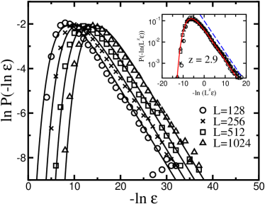
Figure 4: (Color online) Distribution of the log-gaps, identified as the transverse field of the last remaining spin in the RG procedure, for the ladder model with $h_{0}=2.5$ and for different lengths. In the inset a scaling collapse according to Eq.(10) with $z=2.9$ is presented. The Fréchet distributions are indicated by full lines. The asymptotic slope of the curves is indicated by a dashed line and is given by $\omega+1=0.34$, so that the relation in Eq.(21) is well satisfied.

Results of the same analysis of the gaps of the square-lattice RTIM for $h_{0}=9.$ are presented in Fig. 5 for $L=32$, $64$ and $128$. Here the scaling collapse in the inset is obtained with $z=2.7$, whereas the gap exponent is given by $\omega+1=0.74$, so that the localization condition in Eq.(21) is satisfied. Also the Fréchet distribution fits very well the scaled curves.

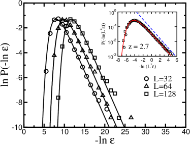
Figure 5: (Color online) The same as in Fig.4 for the square lattice RTIM with $h_{0}=9.$ and for different sizes. In the inset the optimal scaling collapse is obtained with $z=2.7$. The asymptotic slope of the curves is given by $\omega+1=0.74$, so that the relation in Eq.(21) is well satisfied.

II.2.3 Random Heisenberg models in 1d and 2d

The random quantum models studied so far have a discrete symmetry. In this section we are going to consider random Heisenberg models which have continuous symmetry and the renormalization procedure and the corresponding fixed points are somewhat different than for discrete symmetry models. To be specific the Heisenberg models we study here are defined by the Hamiltonian:

$$H_{H}=\sum_{i,j}J_{i,j}t_{i}t_{j}\vec{S}_{i}\cdot\vec{S}_{j}\;,$$ (22)

in terms of spin-$1/2$ variables. $\vec{S}_{i}$ at site, $i$, and the dilution variables: $t_{i}=0$ with probability, $p$, and $t_{i}=1$, otherwise. Here we consider two different types of models. i) For the non-diluted models with $p=0$, the random couplings are both ferromagnetic and antiferromagnetic and their average is $[J]_{\rm av}=0$. ii) For the diluted models we have $0<p<1$ and the random couplings are only antiferromagnetic, $J_{i,j}>0$.

We start with non-diluted models in $1d$ and $2d$ and calculate the smallest gap in the system by the numerical application of the RG method. As described in detail in Ref.lmri03 for these models the RG scales into a so called large spin fixed pointwesterberg , having an effective moment, $S_{eff}\sim L^{d\zeta}$, with $\zeta\approx 1/2$. Due to the formation of large spins the low-temperature singularities of these models are also different than that of the RTIM, for example the average susceptibility has a Curie-like behavior.

The distribution of the log-gaps for the $1d$ non-diluted model is shown in Fig. 6 for different sizes, and in the inset the scaled curves are presented with $z=3.3$. There are considerable deviations from the Fréchet distribution, in particular for small gaps. The relation in Eq.(21) is not satisfied, so that the excitations are non localized.

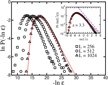
Figure 6: (Color online) Distribution of the log gaps, obtained at the last step of the RG procedure for the $1d$ non-diluted Heisenberg model with uniform disorder, $-0.5<J_{i}<0.5$, and for different sizes. In the inset the optimal scaling collapse is obtained with $z=3.3$. For small gaps there is a considerable deviation from the Fréchet distribution, shown by a full line. The asymptotic slope of the curves is given by $\omega+1=0.67$, so that the relation in Eq.(21) is not satisfied.

The distribution of the log-gaps for the 2d system is shown in Fig. 7 for three sizes, $L=16,~{}32$ and $64$ and in the inset the scaled curves are presented with $z=2$. The Fréchet distribution seems to give a correct description and also the the relation in Eq.(21) is satisfied. We note that in 2d there is frustration in this model, thus it is called as a spin glass.

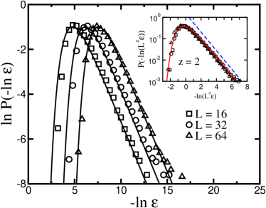
Figure 7: (Color online) The same as in Fig.6 for the square lattice Heisenberg spin glass with Gaussian disorder of variance $1$ for different sizes. In the inset the optimal scaling collapse is obtained with $z=2$. The Fréchet distribution is indicated by a full line and has a satisfactory fit to the data. The asymptotic slope of the curves is given by $\omega+1=1$, so that the relation in Eq.(21) is satisfied.

Next, we consider diluted models on the square lattice for which the couplings are antiferromagnetic and distributed uniformly, $0<J_{i,j}<1$. For the dilution, $p$, we consider two values. In Fig.8 we present the distribution of the gaps at $p=0.125$, which is below the percolation threshold, whereas in Fig.9 we consider the dilution at $p=0.45$, above the percolation threshold, when the system is broken into non-interacting finite clusters.

In the first case during renormalization the system scales into a large spin fixed point. As seen in Fig.8 the distribution of the calculated gaps differs considerably from the Fréchet distribution and also the the relation in Eq.(21) is not correctly satisfied.

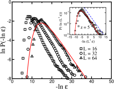
Figure 8: (Color online) The same as in Fig.6 for the square lattice Heisenberg antiferromagnet with dilution $p=0.125$. In the inset the scaling collapse indicates $z=5$. The Fréchet distribution, shown by a full line, differs considerably from the numerical data. The asymptotic slope of the curves is given by $\omega+1=0.35$, so that the relation in Eq.(21) is satisfied only with some error.

For $p=0.45$ the system is separated into independent parts and the smallest gap of the system is just the smallest gap of these clusters. Since the energy gaps of the clusters are expected to be distributed in identical power-law form, the applicability of the EVS is probable. Indeed, in Fig.9 the numerically calculated gap distributions can be well described by the Fréchet form and also Eq.(21) is satisfied.

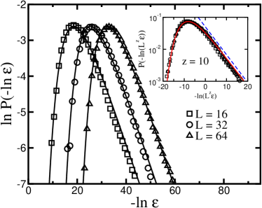
Figure 9: (Color online) The same as in Fig.8 for dilution $p=0.45$, above the percolation threshold. In the inset the optimal scaling collapse is obtained with $z=10$. The Fréchet distributions, indicated by full lines, fit very well the numerical data. The asymptotic slope of the curves is given by $\omega+1=0.2$, so that the relation in Eq.(21) is satisfied.

III Griffiths singularities in random stochastic systems

III.1 PASEP with extreme disorder

First, we consider the PASEP with pw disorder as defined above Eq.(4) with a special form of the bimodal disorder, when the particles are of two kinds. For a fraction of $c\ll 1$ black particles the hopping rates are: $p_{i}=1$ and $q_{i}=\lambda$, whereas the $(1-c)$ fraction of white particles have hopping rates: $p_{i}=1$ and $q_{i}=\lambda^{-1}$. In order to obtain exact results we take the limit $\lambda\gg 1$. With this type of disorder the drift of the white particles to the right is slowed down by the black ones and the slowing dawn is even more effective if two or more black particles happen to stay behind each other. A cluster of $n$ black particles has a very small density: $\rho(n)=c^{n}$ and its speed to the right, in the absence of another black particles and clusters is given by, $v(n)\approx\lambda^{-n}$. Indeed in order to make the complete black cluster one step to the right all the $n$ particles should perform their hop to the unpreferential direction at the same timestep. At this point it is easy to notice the isomorphism of this problem with the RTIM in Sec.II.1.1 with the correspondence: $\epsilon\leftrightarrow v$. Thus we can immediately write for the distribution of the effective velocities of the black clusters:

$$P(v)=\frac{1}{\ln\lambda}v^{\omega},\quad v\to 0\;,$$ (23)

with the exponent, $\omega$, defined in Eq.(8).

Evidently, the stationary velocity of the PASEP is given by the smallest effective speed of the clusters, $v_{1}$, and all the particles move behind that slowest black cluster. In a large finite system with a finite density of particles, the stationary velocity goes to zero as given in Eq.(6) with a dynamical exponent defined in Eq.(9). Consequently in a finite system the distribution of $v_{1}$ is given in the scaling form in Eq.(10), and the distribution function of the scaling variable: $u=u_{0}v_{1}L^{z_{p}}$ is given by the Fréchet distribution in Eq.(11).

The results obtained in this section can be easily generalized for the PASEP with site-wise (sw) disorder, in which case the hop rates depend on the position: for the site $i$ they are $p_{i}$ (right) and $q_{i}$ (left). The control-parameter of the model is the same as for pw disorder in Eq.(4). For the extreme binary disorder considered above most of the sites are white and promote the movement of the particles to the right, but the few black sites and in particular the rare black clusters form barriers, which slow down the particle motion. This problem is studied in more details in Ref.[pasep_sw, ]. Here we just note that the average velocity of a particle which goes trough a single large barrier of size, $n$, is given bybece00 , $v\approx\lambda^{-n/2}$, since due to particle-hole symmetry in the stationary state the barrier is filled up to $n/2$, so that the particles should make $n/2$ consecutive steps against the barrier. As a consequence the derivation in the previous paragraphs for pw disorder should by slightly modified, which leads to a dynamical exponent, $z_{s}$, given by:

$$z_{s}=\frac{z_{p}}{2}\;.$$ (24)

In particular the distribution of the stationary velocity in a finite system is still given by the Fréchet form in terms of the scaling variable: $u=u_{0}v_{1}L^{z_{s}}$.

III.2 Strong disorder RG and scaling results

Here we show that the results in the previous section, i.e the relation between Griffiths singularities and EVS holds for a general form of disorder, too. We start with the PASEP with pw disorder for which a variant of the strong disorder RG approach has been appliedASEP . For this model during renormalization the fastest hop rates are consecutively decimated out and new clusters of particles are created with effective hop rates obtained by a perturbation calculation. Without going to the details we mention that there is a one-to-one correspondence between the RG rules for the RTIM and that of the PASEP. In the Griffiths phase for $\delta_{p}>0$ in the first part of the renormalization both left and right hop rates are decimated out until particle clusters of typical size, $\xi$, are created. (Here $\xi$ is the average correlation length, which behaves for small $\delta_{p}$ as $\xi\sim\delta_{p}^{-2}$.) At this scale of the RG the remaining effective particles have a practically vanishing left hop rate, $\tilde{q}_{i}\approx 0$, and finite effective right hop rates, which have an asymptotic power-law distribution: $P(\tilde{p})\sim\tilde{p}^{-1+1/z_{p}}$. Here the dynamical exponent, $z_{p}$, is given through the equation:

$$\left[\left(\frac{q}{p}\right)^{1/z_{p}}\right]_{\rm av}=1\;,$$ (25)

which makes the analogy with the RTIM complete, see in Eq.(14). The renormalized PASEP than consists of independent particles the velocity (right hop rate) of them has the same power-law distribution and the smallest of them is the stationary velocity of the finite system. Consequently the conditions of EVS are asymptotically satisfied, so that the distribution of the stationary velocity in a finite system is given by the Fréchet form in terms of the scaling variable: $u=u_{0}v_{1}(L/\xi)^{z_{p}}$.

For the PASEP with sw disorder one can not simply apply the strong disorder RG, so that we use here phenomenological, scaling considerations. As noticed in Sec.III.1 the rare regions are represented by large barriers, which in the length-scale, $\xi$, are expected to be independent and well separated from each other. Scaling consideration in Ref.[ASEP, ] show that the distribution of the velocities associated to large barriers is given by, $P(v)\sim v^{-1+1/z_{s}}$ and for the dynamical exponent, $z_{s}$, the relation in Eq.(24) holds in the entire Griffiths phase. Once more the stationary velocity in a finite system is given by the smallest velocity associated to the largest barrier, and its distribution is expected to be in the Fréchet form in terms of the scaling variable: $u=u_{0}v_{1}(L/\xi)^{z_{s}}$.

Finally, we consider the 1d zero-range process (ZRP) with quenched disorderZRP . In this model the $i$-th lattice site can be occupied by $n_{i}\geq 0$ particles, from which the topmost one can hop to nearest neighbor sites with a position dependent rate: $q_{i}$ to site $i+1$ and $p_{i-1}$ to site $i-1$. It is known that the ZRP with this definition can be exactly mapped (up to translations of the configurations of the lattice) to the PASEP with pw disorder, as studied here. The sites of the ZRP are particles in the ASEP and the particle clusters in the ZRP correspond to holes in front of the particles in the PASEP. Then the stationary current in the ZRP is just the stationary particle velocity of the PASEP. From this mapping and the previous reasoning follows that the stationary current of the ZRP, $J$, in a finite system scales as: $J\sim L^{-z_{p}}$, and its distribution is the Fréchet distribution.

III.3 Numerical results

We start to analyze the distribution of the stationary velocity, $v$, of the PASEP with uniform pw disorder, which is presented in Fig.10. Here we have evaluated an exact expression for $v$, which is described c.f. in Ref.[ASEP, ] and in this way we have studied chains with up to $N=2048$ particles over 100000 independent realizations of the disorder. Fig.10 shows an excellent agreement with the Fréchet distribution having the exact dynamical exponent in Eq.(25).

Figure 10: Distribution of the stationary velocity of the PASEP with pw uniform disorder having $h_{0}=3.$ calculated for different numbers of particles. The Fréchet distribution with the exact dynamical exponent in Eq.(25) is indicated by the full line.

For the PASEP with sw disorder there is no analytical expression for the stationary velocity so that $v$ is calculated by simulation. We have considered 10000 random half-filled chains with binary disorder of different lengths up to $L=512$. The results as presented in Fig.11 are in good agreement with the Fréchet distribution, in which the exact dynamical exponent is taken from the scaling result in Eqs.(24) and (25).

Figure 11: The same as in Fig.10 for the PASEP sw binary disorder with $c=0.25$ and $\lambda=2.$ For the Fréchet distribution, which is indicated by the full line the dynamical exponent is taken from the scaling result in Eqs.(24) and (25).

IV Discussion

In this paper we have considered strong Griffiths effects in different interacting many particle systems and studied their possible relation with extreme value statistics. Our examples included random quantum systems in one and two dimensions as well as stochastic systems with quenched disorder in one dimension. Our exact, numerical and RG results indicate that for systems having a discrete symmetry the distribution of the inverse time scales (excitation energy for quantum systems, stationary velocity for exclusion models) in large finite samples has a universal form, which is the limit distribution of the extremes of iid random numbers. In these examples the Griffiths singularities are characterized by the dynamical exponent, $z$, which is a continuous function of the control parameter, $\delta$. However the distribution function depends on, $u=L^{z/d}\tau^{-1}$, and given by the Fréchet distribution in Eq.(11). The physical picture behind this result is given by the strong disorder RG method: during renormalization fast degrees of freedom are gradually decimated out and the system finally transforms into a set of practically independent degrees of freedom. The characteristic time-scales of these localized units follow a power-law distribution with a $z$-dependent decay exponent. Since the physically relevant relaxation time is given by the largest time-scale we arrive to the results of EVS.

The universality of the distribution function of different problems is tested by numerical and RG calculations. For models with a discrete symmetry in all cases we obtained convincing evidence of universality. On the contrary for the random Heisenberg model, which has a continuous symmetry, the distribution function is found to depend on the specific form of the disorder. Interestingly, for the 2d spin-glass model as well as for the diluted 2d model above the percolation threshold the distribution function is found in universal Fréchet form.

One might ask the question how general these results are. On the basis of the RG approach we conjecture that for all interacting systems which have a disordered Griffiths phase the singular properties of which are controlled by the same type of strong disorder fixed points as for the RTIM the distribution function of the inverse time-scales is universal. Possible systems of this class are, besides random quantum magnets and exclusion processes, some reaction-diffusion modelscontact , the dynamics of the random-field Ising chainrfim , the localization of a random polymer at an interfacepolymer , etc.

Evidently the above considerations of EVS does not apply for the distribution of average and local physical quantities in random systems. For the RTIM average quantities are, among others the uniform susceptibility or the sound velocityluck , whereas examples for local quantities are the surface susceptibility or the surface magnetization in the ordered Griffiths phasebigpaper ; dharyoung ; cecile . The biased random walk in a random environmentwalk is a one particle problem, thus the applicability of the EVS is not expected. Indeed, the stationary velocity is an average quantity, since the time needed for the particle to get through a system is obtained by averaging the waiting times associated at different points of the latticederrida . Therefore the distribution of the stationary velocity is not in the Fréchet formwalk .

- (1) R. B. Griffiths, Phys. Rev. Lett. 23, 17 (1969).
- (2) A. B. Harris, Phys. Rev. B12, 203 (1975).
- (3) For reviews, see: H. Rieger and A. P Young, in Complex Behavior of Glassy Systems, ed. M. Rubi and C. Perez-Vicente, Lecture Notes in Physics 492, p. 256, Springer-Verlag, Heidelberg, 1997; R. N. Bhatt, in Spin glasses and random fields A. P. Young Ed., World Scientific (Singapore, 1998).
- (4) D.S. Fisher, Phys. Rev. Lett. 69, 534 (1992); Phys. Rev. B 51, 6411 (1995).
- (5) B. McCoy, Phys. Rev. Lett. 23, 383 (1969).
- (6) G.M. Schütz, “Integrable Stochastic many-body systems” in Phase Transitions and Critical Phenomena, vol. 19, Eds. C. Domb and J.L. Lebowitz (Academic Press, San Diego, 2001).
- (7) J. Krug, Braz. J. Phys. 30, 97 (2000).
- (8) R. Juhász, L. Santen, and F. Iglói, Phys. Rev. Lett. 94, 010601 (2005).
- (9) R. Juhász, L. Santen, and F. Iglói, (unpublished)
- (10) R. Juhász, L. Santen, and F. Iglói, Phys. Rev. E 72, 046129 (2005)
- (11) H. Hinrichsen, Adv. Phys. 49, 815 (2000).
- (12) J. Hooyberghs, F. Iglói, and C. Vanderzande Phys. Rev. Lett. 90, 100601 (2003); Phys. Rev. E 69, 066140 (2004).
- (13) Th. Vojta, and M. Dickison, Phys. Rev. E 72, 036126 (2005).
- (14) G. Ódor, and N. Menyhárd, preprint cond-mat/0512252.
- (15) J. Galambos, The Asymptotic Theory of Extreme Order Statistics (John Wiley and Sons, New York, 1978).
- (16) G. Györgyi, P. C. Holdsworth, B. Portelli, and Z. Rácz, Phys. Rev. E68, 056116 (2003).
- (17) D.S. Dean and S.N. Majumdar, Phys. Rev. E 64, 046121 (2001).
- (18) For a review, see: F. Iglói and C. Monthus, Physics Reports 412, 277, (2005).
- (19) This scaling form in the general case follows from the assumption that the rare regions are localized, thus for a small we have . A.P. Young and H. Rieger, Phys. Rev. B 53, 8486 (1996).
- (20) S.-K. Ma, C. Dasgupta, and C.-k. Hu, Phys. Rev. Lett. 43, 1434 (1979); C. Dasgupta and S.-K. Ma, Phys. Rev. B 22, 1305 (1980).
- (21) F. Iglói, R. Juhász, and P. Lajkó, Phys. Rev. Lett. 86, 1343 (2001).
- (22) F. Iglói, Phys. Rev. B 65, 064416 (2002).
- (23) F. Iglói and H. Rieger, Phys. Rev. E58, 4238 (1998).
- (24) D.S. Fisher and A. P. Young, Phys. Rev. B 58, 9131 (1998).
- (25) O. Motrunich, K. Damle and D.A. Huse, Phys. Rev. B 63 134424 (2001).
- (26) F. Iglói and H. Rieger Phys. Rev. B 57 11404 (1998).
- (27) F. Iglói, R. Juhász and H. Rieger, Phys. Rev. B59, 11308 (1999).
- (28) O. Motrunich, S.-C. Mau, D. A. Huse, and D. S. Fisher, Phys. Rev. B 61, 1160 (2000).
- (29) Y-C. Lin, N. Kawashima, F. Iglói and H. Rieger, Progress in Theor. Phys. (Suppl.) 138, 479 (2000).
- (30) T. Senthil and S. N. Majumdar, Phys. Rev. Lett. 76, 3001 (1996).
- (31) At the particular value, , the RG equations are equivalent to that of the dimerized random antiferromagnetic Heisenberg chain, given in Eq.(22) with and with different antiferromagnetic couplings at odd and even bonds, see in Ref.ijl .
- (32) R. Juhász, PhD thesis, Szeged University (2003) (unpublished).
- (33) Y.-C. Lin, R. Mélin, H. Rieger, and F. Iglói, Phys. Rev. B 68, 024424 (2003).
- (34) E. Westerberg, A. Furusaki, M. Sigrist, and P.A. Lee, Phys. Rev. Lett. 75 4302 (1995); E. Westerberg, A. Furusaki, M. Sigrist, and P.A. Lee, Phys. Rev. B55, 12578 (1997).
- (35) R. A. Blythe, M. R. Evans, F. Colaiori, and F. H. L. Essler, J. Phys. A33, 2313 (2000).
- (36) D. S. Fisher, P. Le Doussal and C. Monthus, Phys. Rev. E64, 66107 (2001).
- (37) C. Monthus, Eur. Phys. J. B13, 111 (2000).
- (38) J.M. Luck, J. Stat. Phys. 72, 417 (1993).
- (39) A. Dhar and A.P. Young, Phys. Rev. B68, 134441 (2003).
- (40) C. Monthus, Phys. Rev. B69, 054431 (2004).
- (41) D. S. Fisher, P. Le Doussal and C. Monthus, Phys. Rev. E 59, 4795 (1999).
- (42) B. Derrida, J. Stat. Phys. 31, 433 (1983).