Lattice Distortion and Magnetism of $3d$-$t_{2g}$ Perovskite Oxides

Abstract

Several puzzling aspects of interplay of the experimental lattice distortion and the the magnetic properties of four narrow $t_{2g}$-band perovskite oxides (YTiO₃, LaTiO₃, YVO₃, and LaVO₃) are clarified using results of first-principles electronic structure calculations. First, we derive parameters of the effective Hubbard-type Hamiltonian for the isolated $t_{2g}$ bands using newly developed downfolding method for the kinetic-energy part and a hybrid approach, based on the combination of the random-phase approximation and the constraint local-density approximation, for the screened Coulomb interaction part. Apart form the above-mentioned approximation, the procedure of constructing the model Hamiltonian is totally parameter-free. The results are discussed in terms of the Wannier functions localized around transition-metal sites. The obtained Hamiltonian was solved using a number of techniques, including the mean-field Hartree-Fock (HF) approximation, the second-order perturbation theory for the correlation energy, and a variational superexchange theory, which takes into account the multiplet structure of the atomic states. We argue that the crystal distortion has a profound effect not only on the values of the crystal-field (CF) splitting, but also on the behavior of transfer integrals and even the screened Coulomb interactions. Even though the CF splitting is not particularly large to quench the orbital degrees of freedom, the crystal distortion imposes a severe constraint on the form of the possible orbital states, which favor the formation of the experimentally observed magnetic structures in YTiO₃, YVO₃, and LaVO₃ even at the level of mean-field HF approximation. It is remarkable that for all three compounds, the main results of all-electron calculations can be successfully reproduced in our minimal model derived for the isolated $t_{2g}$ bands. We confirm that such an agreement is only possible when the nonsphericity of the Madelung potential is explicitly included into the model. Beyond the HF approximation, the correlations effects systematically improve the agreement with the experimental data. Using the same type of approximations we could not reproduce the correct magnetic ground state of LaTiO₃. However, we expect that the situation may change by systematically improving the level of approximations for dealing with the correlation effects.

I Introduction

The transition-metal perovskite oxides $AB$O₃ (with $A$$=$ Y, La, or other trivalent rare-earth ion, and $B$$=$ Ti or V) are regarded as some of the key materials for understanding the strong coupling among spin, orbital, and lattice degrees of freedom in correlated electron systems.reviews

According to the electronic structure calculations in the local-density approximation (LDA), all these compounds can be classified as “$t_{2g}$ systems”, as all of them have a common transition-metal $t_{2g}$-band, located near the Fermi level, which is well separated from the oxygen-$2p$ band and a hybrid transition-metal $e_{g}$ and either Y($4d$) or La($5d$) band, located correspondingly in the lower- and upper-part of the spectrum (Fig. 1).

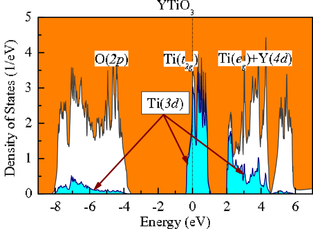
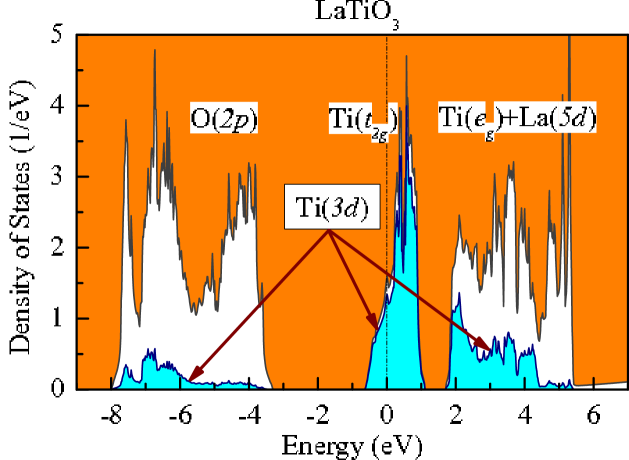
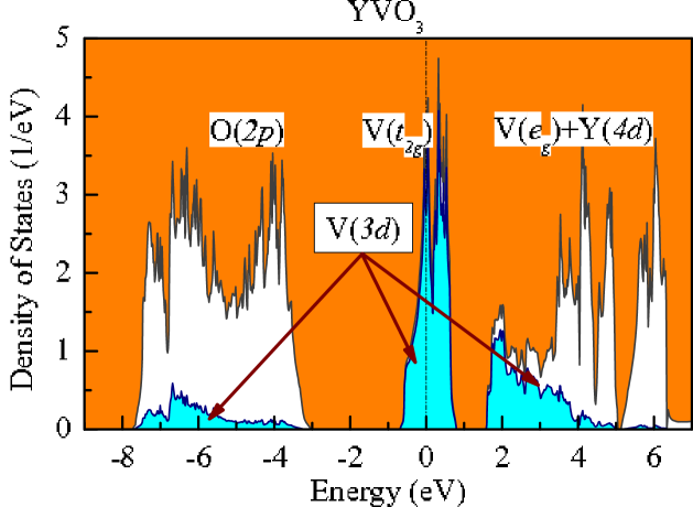
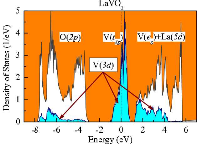
Figure 1: (Color online) Total and partial densities of states for YTiO₃, LaTiO₃, YVO₃ (orthorhombic phase), and LaVO₃ in the local-density approximation. The shaded area shows the contributions of the transition-metal $3d$-states. Other symbols show positions of the main bands. The Fermi level is at zero energy.

The number of electrons that are donated by each Ti and V site into the $t_{2g}$-band is correspondingly one and two. These electrons are subjected to the strong intraatomic Coulomb repulsion, which is not properly treated by LDA and requires some considerable improvement of this approximation, which currently processes in the direction of merging LDA with various model approaches for the strongly-correlated systems.AZA ; PRB94 ; LSDADMFT ; Imai Nevertheless, LDA continues play an important role for these systems as it naturally incorporates into the model analysis the effects of the lattice distortion, and does it formally without any adjustable parameters. Although the origin of the lattice distortion in the $t_{2g}$ perovskite oxides is not fully understood, is is definitely strong and exhibits an appreciable material-dependence, which can be seen even visually in Fig. 2.

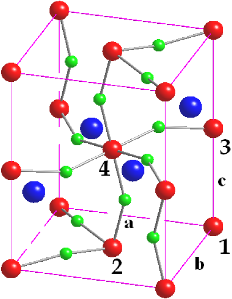
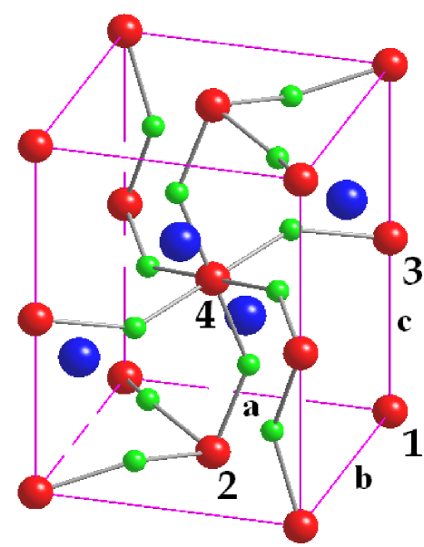
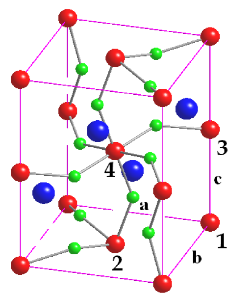
Figure 2: (Color online) Crystal structure of orthorhombic LaTiO₃ (left), YTiO₃ (middle), and YVO₃ (right). La and Y sites are indicated by big blue spheres, Ti and V sites – by medium red spheres, and oxygen sites – by small green spheres. The symbols ${\bf a}$, ${\bf b}$, and ${\bf c}$ stand for the orthorhombic translations. The symbols $1$-$4$ denote the transition-metal sites, which forms the unit cell of the distorted perovskite oxides.

The interplay of this lattice distortion with the Coulomb correlations seems to be the key factor for understanding the large variation of the magnetic properties among the $t_{2g}$ perovskite oxides. The difference exists not only between Ti- and V-based compounds, but also within each group of formally isovalent materials, depending on whether it is composed of the Y or La atoms. The latter seems to be a clear experimental manifestation of the distortion effect, which is related with the difference of the ionic radii of Y and La. All together this leads to the famous phase diagram of the distorted $t_{2g}$ perovskite oxides, where each material exhibits quite a distinct magnetic behavior: YTiO₃ is a ferromagnet;Maclean ; Itoh ; Akimitsu ; Ulrich2002 ; Iga LaTiO₃ is a three-dimensional (G-type) antiferromagnet;Keimer ; Cwik YVO₃ has the low-temperature G-type antiferromagnetic (AFM) phase, which at around $77$ K transforms into a chain-like (C-type) antiferromagnetic phase;Ren ; Blake ; Tsvetkov ; Ulrich2003 and LaVO₃ is the C-type antiferromagnet.Zubkov ; Bordet

On the theoretical side, the large variety of these magnetic phases has been intensively studied using model approaches (Refs. MizokawaFujimori, ; KhaliullinMaekawa, ; Khaliullin01, ; Khaliullin02, ; MochizukiImada, ; Schmitz, ) as well as the first-principles electronic structure calculations (Refs. FujitaniAsano, ; Sawada96, ; SawadaTerakura, ; PRB04, ; FangNagaosa, ; Pavarini1, ; Pavarini2, ; Streltsov, ; Okatov, ). The problem is still far from being understood, and remains to be the subject of numerous contradictions and debates. Surprisingly that at present there is no clear consensus not only between model and first-principles electronic structure communities, but also between researchers working in each of these groups. Presumably, the most striking example is LaTiO₃, where in order to explain the experimentally observed G-type AFM ground state, two different models, which practically exclude each other, have been proposed. One is the model of orbital liquid, which implies the degeneracy of the atomic $t_{2g}$ levels in the crystalline environment.KhaliullinMaekawa Another model is based on the theory of crystal-field (CF) splitting, which lifts the orbital degeneracy and leads to the one particular type the orbital ordering compatible with the G-type antiferromagnetism.MochizukiImada ; Schmitz The situation in the area of first-principles electronic structure calculations is controversial as well. Although majority of the researchers now agree that in order to describe properly the electronic structure of $t_{2g}$ perovskite oxides, one should go beyond the conventional LDA and incorporate the effects of intraatomic Coulomb correlations, this merging is typically done in a semi-empirical way, as it relies on a certain number of adjustable parameters, postulates, and the form of the basis functions used for the implementation of various corrections on the top of LDA.AZA ; PRB94 ; LSDADMFT There are also certain differences regarding both the definition and the approximations used for the CF splitting in the electronic structure calculations, which will be considered in details in Sec. III.1. Since the magnetic properties of $t_{2g}$ perovskite oxides are extremely sensitive to all such details, it is not surprising that there is a substantial variation in the results of first-principles calculations, which sometimes yield even qualitatively different conclusions about the CF splitting and the magnetic structure of the distorted $t_{2g}$ perovskite oxides.PRB04 ; Pavarini2 ; Streltsov ; Okatov These discrepancies put forward a severe demand on the creation of a really parameter-free scheme of electronic structure calculations for the strongly-correlated systems.

Therefore, the main motivation of the present work is twofold.
(i) In our previous work (Ref. condmat05, ) we have proposed a method of construction of the effective Hubbard-type model for the electronic states near the Fermi level on the basis of first-principles electronic structure calculations. In the present work we apply this strategy to the $t_{2g}$ states of the distorted perovskite oxides. Namely, we will derive the parameters of the Hubbard Hamiltonian for the $t_{2g}$ bands and solve this Hamiltonian using several different techniques, including the Hartree-Fock (HF) approximation, the perturbation theory for the correlation energy, and the the theory of superexchange interactions taking into account the effects of the multiplet structure of the atomic states. Of course, our method is based on a number of approximation, which have been introduced in Ref. condmat05, and will be briefly discussed in Sec. III. However, we would like to emphasize from the very beginning that our policy here is not to use any adjustable parameters apart from the approximations considered in Ref. condmat05, . Thus, we believe that it poses a severe test for the proposed method, and the obtained results should clearly demonstrate that our general strategy, which can be expressed by the formula first-principles electronic structure calculations $\rightarrow$ construction of the model Hamiltonian $\rightarrow$ solution of the model Hamiltonian,Imai ; condmat05 is indeed very promising. For example, at the HF level, using relatively simple model Hamiltonian, which is limited exclusively by the $t_{2g}$ bands, we will be able to reproduce the main results of all-electron calculations.SawadaTerakura ; FangNagaosa Furthermore, due to the simplicity of the model Hamiltonian we can easily go beyond the HF approximation and include the correlation effects.
(ii) Why do we need to convert the results of first-principles electronic structure calculations into a model? Apart from the purely computational reason, related with the reduced dimensionality of the Hilbert space for the solution of the many-electron problem,Imai the story of distorted $t_{2g}$ perovskite oxides clearly shows that the model consideration has yet another advantage, which is typically not sufficiently appreciated in the computational community. It is true that the field of first-principles electronic structure calculations is currently on the rise, and the calculation of the basic properties for many materials will soon become a matter of routine. However, the methods of electronic structure calculations are based on some approximations, the limitations of which should be clearly understood. Furthermore, like the experiment data, the results of first-principles electronic structure calculations will always require some interpretation, which would transform the world of numbers and trends into a “parallel world” of rationalized model categories capturing the essence of the electronic structure calculations. The understanding of the results of calculations in terms of these categories opens a way, on the one hand, to the material engineering of compounds with a desired set of properties, and, on the other way, to “engineering” of the new methods of electronic structure calculations in the direction of elucidation and overcoming the existing approximations. In this work we will illustrate how the results of first-principles calculations for the distorted perovskite oxides can be interpreted in terms of a limited number of model parameters, such as the crystal-field splitting, transfer integrals, and the intraatomic Coulomb interactions, which can be regarded as the basic operating blocks for understanding the properties of these materials as well as the limitation of approximations existing in the methods of electronic structure calculations. Particularly, we will explicitly show that the atomic-spheres-approximation (ASA), which was employed in the series of publications (Refs. PRB04, ; Pavarini1, ; Pavarini2, ; Streltsov, ), is not enough as it neglects the nonsphericity of the Madelung potential. The latter plays an important role and in many cases predetermines the character of the magnetic ordering in the distorted $t_{2g}$ perovskite oxides. We will also show that once the parameters of Coulomb interactions are determined from the first principles, the commonly used mean-field HF approximation does not necessary guaranty the right answer for the magnetic properties of $t_{2g}$ perovskite oxides. However, we will argue that this is a normal situation, and in the majority of cases, a better agreement with the experimental data can be obtained by systematically including the correlation effects beyond the HF approximation. In this sense, our strategy is completely different from conventional LDA$+$$U$ calculations, where the on-site Coulomb interaction $U$ is typically treated as an adjustable parameter (e.g., Refs. SawadaTerakura, ; FangNagaosa, ; Pavarini2, ; Streltsov, ; Okatov, ). By changing $U$, one can certainly get a better numerical agreement with some experimental data already at the HF level. However, one should clearly understand that such an empirical treatment actually disguises the actual role played by the correlation effects in the narrow-band compounds.

The rest of the paper is organized as follows. In Sec. II we will briefly remind the main details of the crystal and magnetic structure of the distorted perovskite oxides. The procedure of constructing the model Hamiltonian as well as the results of calculations of the CF splitting, transfer integrals, and on-site Coulomb interactions for the isolated $t_{2g}$ band will be briefly explained in Sec. III. Particularly, in Sec. III.1 we will discuss highly controversial situation around the values of the CF splitting extracted from electronic structure calculations,PRB04 ; Pavarini1 ; Pavarini2 ; Streltsov and argue that the main difference is caused by two factors: (i) certain arbitrariness with the choice of the Wannier functions for the $t_{2g}$ bands of the distorted perovskite oxides; (ii) additional approximations used for the nonspherical part of the crystalline potential inside atomic spheres. The methods of solution of the model Hamiltonian will be described Sec. IV, and the results of calculations will be presented in Sec. V. Finally, in Sec. VI we will summarize the main results of our work.

II Crystal and Magnetic Structures

The distorted perovskite oxides contain four formula units in the primitive cell. The transition-metal ($B$) atoms are located at $(0,0,0)$ (site 1), $({\bf a}/2,{\bf b}/2,0)$ (site 2), $(0,0,{\bf c}/2)$ (site 3), and $({\bf a}/2,{\bf b}/2,{\bf c}/2)$ (site 4), in terms of three primitive translations: ${\bf a}$, ${\bf b}$, and ${\bf c}$ (see Fig. 2). The distortion can be either orthorhombic or monoclinic.

The space group of the orthorhombic phase is $D^{16}_{2h}$ (in the Schönflies notations or $Pbnm$ in the Hermann-Maguin notations, No. 62 in the International Tables). In this case all $B$-sites are equivalent and can be transformed to each other using symmetry operations of the $D^{16}_{2h}$ group.

The monoclinic phase has the space group $C^{5}_{2h}$ ($P2_{1}/a$, No. 14 in the International Tables).Blake ; comment.7 In this case, there are two nonequivalent pairs of $B$-sites: (1,2) and (3,4). Each pair is allocated within the same ${\bf ab}$-plane, so that the atoms can be transformed to each other using symmetry operations of the $C^{5}_{2h}$ group. However, there is no symmetry operation, which connects the atoms belonging to different ${\bf ab}$-planes.

We use the experimental lattice parameters and the atomic positions reported in Ref. Maclean, for YTiO₃ (the data corresponds to the temperature T$=$$293$ K), in Ref. Cwik, for LaTiO₃ (T$=$$8$ K), in Ref. Blake, for YVO₃ (T$=$$65$ K and $100$ K, for the orthorhombic and monoclinic phase, respectively), and in Ref. Bordet, for LaVO₃ (T$=$$10$ K).

There are five possible magnetic structure, which can be obtained by associating with each transition-metal site either positive ($\uparrow$) or negative ($\downarrow$) direction of spin, without enlarging the unit cell. Therefore, each magnetic structure can be denoted by means of four vectors associated with the transition-metal sites (1 2 3 4). They are
1. ($\uparrow$$\uparrow$$\uparrow$$\uparrow$), which is called the ferromagnetic (F) phase;
2. ($\uparrow$$\uparrow$$\downarrow$$\downarrow$), the layered (A-type) antiferromagnetic phase;
3. ($\uparrow$$\downarrow$$\uparrow$$\downarrow$), the chainlike (C-type) antiferromagnetic phase;
4. ($\uparrow$$\downarrow$$\downarrow$$\uparrow$), the totally antiferromagnetic (G-type) phase;
5. ($\downarrow$$\uparrow$$\uparrow$$\uparrow$), the spin-flip phase. In the monoclinic structure, there are two different spin-flip phases: ($\downarrow$$\uparrow$$\uparrow$$\uparrow$) and ($\uparrow$$\uparrow$$\downarrow$$\uparrow$), which will be denoted as flip-I and flip-II, respectively.
Similar classification can be used the orbital ordering. Typically, two orthogonal orbitals at the neighboring transition-metal sites are said to be ordered antiferromagnetically, although such a definition is not unique.comment.6

III Model Hamiltonian

Our first goal is the construction of the effective multi-orbital Hubbard model for the isolated $t_{2g}$ bands:

$$\hat{\cal{H}}=\sum_{{\bf R}{\bf R}^{\prime}}\sum_{\alpha\beta}h_{{\bf R}{\bf R}^{\prime}}^{\alpha\beta}\hat{c}^{\dagger}_{{\bf R}\alpha}\hat{c}^{\phantom{\dagger}}_{{\bf R}^{\prime}\beta}+\frac{1}{2}\sum_{\bf R}\sum_{\alpha\beta\gamma\delta}U_{\alpha\beta\gamma\delta}\hat{c}^{\dagger}_{{\bf R}\alpha}\hat{c}^{\dagger}_{{\bf R}\gamma}\hat{c}^{\phantom{\dagger}}_{{\bf R}\beta}\hat{c}^{\phantom{\dagger}}_{{\bf R}\delta},$$ (1)

where $\hat{c}^{\dagger}_{{\bf R}\alpha}$ ($\hat{c}_{{\bf R}\alpha}$) creates (annihilates) an electron in the Wannier orbital $\tilde{W}_{\bf R}^{\alpha}$ of the site ${\bf R}$, and $\alpha$ is a joint index, incorporating all remaining (spin and orbital) degrees of freedom. The matrix $\hat{h}_{{\bf R}{\bf R}^{\prime}}$$=$$\|h_{{\bf R}{\bf R}^{\prime}}^{\alpha\beta}\|$ parameterizes the kinetic energy of electrons, where the site-diagonal part (${\bf R}$$=$${\bf R}^{\prime}$) describes the local level-splitting, caused by the crystal field and (or) the spin-orbit interaction, and the off-diagonal part (${\bf R}$$\neq$${\bf R}^{\prime}$) stands for the transfer integrals. $U_{\alpha\beta\gamma\delta}=\int d{\bf r}\int d{\bf r}^{\prime}\tilde{W}_{\bf R}^{\alpha\dagger}({\bf r})\tilde{W}_{\bf R}^{\beta}({\bf r})v_{\rm scr}({\bf r}$$-$${\bf r}^{\prime})\tilde{W}_{\bf R}^{\gamma\dagger}({\bf r}^{\prime})\tilde{W}_{\bf R}^{\delta}({\bf r}^{\prime})\equiv\langle\tilde{W}_{\bf R}^{\alpha}\tilde{W}_{\bf R}^{\gamma}|v_{\rm scr}|\tilde{W}_{\bf R}^{\beta}\tilde{W}_{\bf R}^{\delta}\rangle$ are the matrix elements of screened Coulomb interaction $v_{\rm scr}({\bf r}$$-$${\bf r}^{\prime})$, which are supposed to be diagonal with respect to the site indices.

The parameters of the Hubbard Hamiltonian (1) can be derived “from the first principles”, starting from the electronic structure in LDA. This procedure has been already discussed in details in Ref. condmat05, . Here we only remind the main ideas and present the results for the distorted perovskite compounds.

All calculations have been performed using linear muffin-tin-orbital (LMTO) method in the atomic-spheres-approximation.LMTO We have also considered the additional correction to the crystal-field splitting, coming from the nonsphericity of electron-ion interactions, beyond conventional ASA.condmat05

III.1 Kinetic-Energy Part, Controversy about the Crystal-Field Splitting

The kinetic-energy part of the Hubbard Hamiltonian was constructed using the downfolding method.condmat05 ; PRB04 It yields certain set of parameters $\{h_{{\bf R}{\bf R}^{\prime}}^{\alpha\beta}\}$. The Wannier functions $\{\tilde{W}_{\bf R}^{\alpha}\}$ for the the isolated $t_{2g}$ bands can be formally reconstructed from $\{h_{{\bf R}{\bf R}^{\prime}}^{\alpha\beta}\}$ using the definition $h_{{\bf R}{\bf R}^{\prime}}^{\alpha\beta}$$=$$\langle\tilde{W}_{\bf R}^{\alpha}|\hat{H}^{\rm LDA}|\tilde{W}_{\bf R}^{\beta}\rangle$, where $\hat{H}^{\rm LDA}$ is the LDA Hamiltonian in ASA.comment.2

The (characteristic) example of such Wannier functions constructed for LaTiO₃ is shown in Fig. 3,

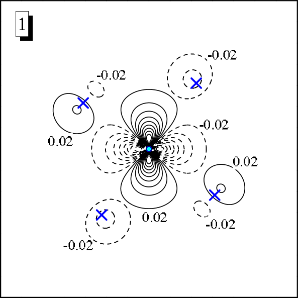
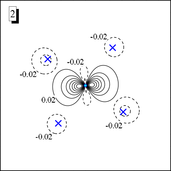
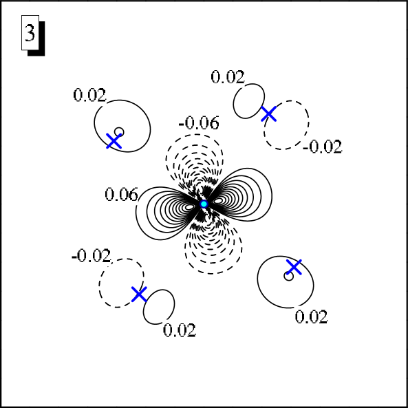
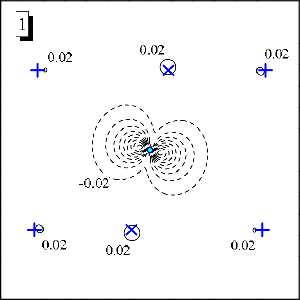
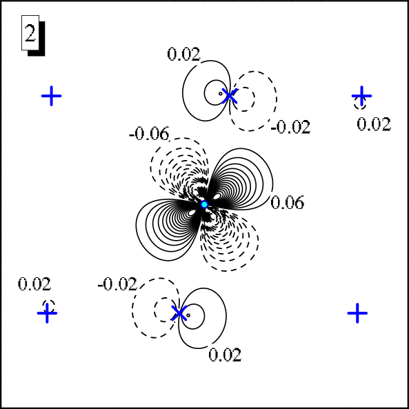
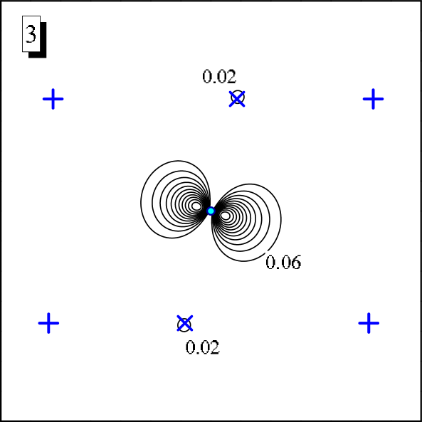
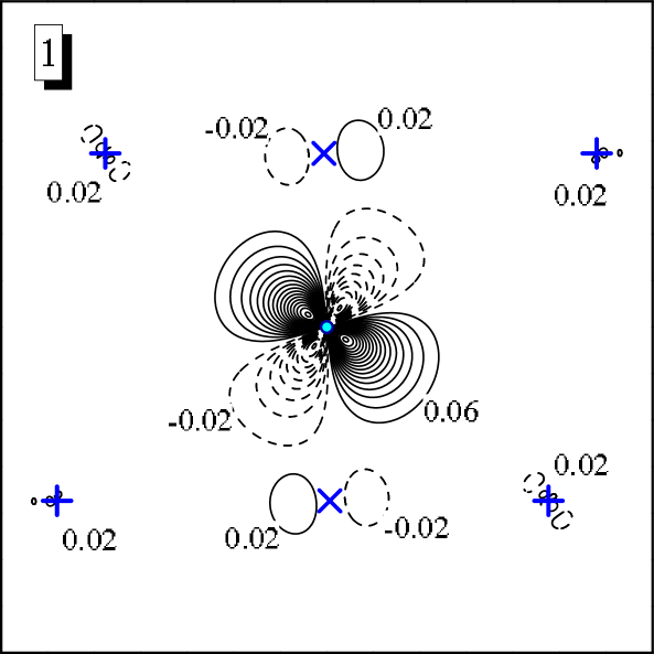
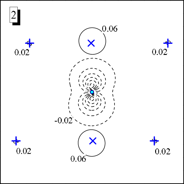
Figure 3: (Color online) Contour plot of the Wannier functions in the case of LaTiO₃ in three orthorhombic planes: ${\bf ab}$ (top), ${\bf ac}$ (middle), and ${\bf bc}$ (bottom). The solid and dashed line correspond to the positive and negative values of the Wannier functions. The projections of different atoms on the planes are denoted by the following symbols: $+$ (La), $\circ$ (Ti), and $\times$ (O). Around each site, the Wannier function increases/decreses with the step $0.04$ from the values indicated on the graph.

and their extension in the real space is illustrated in Fig. 4.

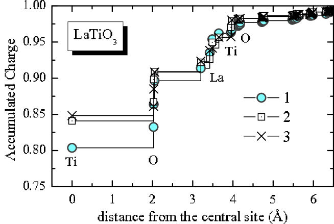
Figure 4: Spacial extension of the Wannier functions in the case of LaTiO₃: the electronic charge accumulated around the central Ti site after adding every new sphere of neighboring atomic sites.

The functions are well localized: about 80-85% of their total weight is concentrated at the central Ti site, 5-9 % belong to neighboring oxygen sites, and about 10 % is distributed over La, Ti, and O sites located in next coordination spheres. Another measure of localization of the Wannier functions is the expectation value of the square of the position operator: $\langle{\bf r}^{2}\rangle_{\alpha}$$=$$\langle\tilde{W}_{\bf R}^{\alpha}|({\bf r}$$-$${\bf R})^{2}|\tilde{W}_{\bf R}^{\alpha}\rangle$,MarzariVanderbilt which yields $\langle{\bf r}^{2}\rangle_{\alpha}$$=$ $2.68$, $2.36$, and $2.37$ Å² for $\alpha$$=$ 1, 2, and 3, respectively. The Wannier functions for LaTiO₃ are less localized in comparison with the more distorted YTiO₃, where $\langle{\bf r}^{2}\rangle$ is of the order of $1.90$-$2.28$ Å².condmat05 However, this is to be expected.

The parameters $\{h_{{\bf R}{\bf R}^{\prime}}^{\alpha\beta}\}$ include all kinds of hybridization (or covalent mixing) effects between transition-metal $t_{2g}$ and other atomic orbitals. However, there are other effects, which are not yet included in $\{h_{{\bf R}{\bf R}^{\prime}}^{\alpha\beta}\}$. They come from the nonsphericity (n-s) of the Madelung potential for the electron-ion interactions, and contribute to the CF splitting. The proper correction to $\{h_{{\bf R}{\bf R}^{\prime}}^{\alpha\beta}\}$ can be easily calculated in the basis of Wannier functions $\{\tilde{W}_{\bf R}^{\alpha}\}$:

$$\Delta^{\rm n-s}h_{\bf RR}^{\alpha\beta}=\sum_{{\bf R}^{\prime}\neq{\bf R}}\langle\tilde{W}_{\bf R}^{\alpha}|\frac{-Z^{*}_{{\bf R}^{\prime}}e^{2}}{|{\bf R}+{\bf r}-{\bf R}^{\prime}|}|\tilde{W}_{\bf R}^{\beta}\rangle,$$ (2)

where $Z^{*}_{{\bf R}^{\prime}}$ is the total charge associated with the site ${\bf R}^{\prime}$ (namely, the nuclear charge minus the screening electronic charge encircled by the atomic sphere), and ${\bf r}$ is the position of the electron in the sphere ${\bf R}$.

The main idea behind this treatment of the CF splitting is based on certain hierarchy of interactions in solids. It implies that the strongest interaction, which leads to the energetic separation of the $t_{2g}$ band from other bands (Fig. 1), is the covalent mixing. For example, in many transition-metal oxides this interaction is mainly responsible for the famous splitting between the transition-metal $t_{2g}$ and $e_{g}$ states.Kanamori1 The nonsphericity of the Madelung potential is considerably weaker than this splitting. However, it can be comparable with the effects of covalent mixing in the narrow $t_{2g}$ band. Therefore, the basic idea is to treat this nonsphericity as a pseudo-perturbation,LMTO and calculate the matrix elements of the Madelung potential in the basis of Wannier functions constructed for spherically averaged ASA potential.

The same strategy can be used for the spin-orbit (s-o) interaction, which yields the following correction to the kinetic part of the model Hamiltonian:

$$\Delta^{\rm s-o}h_{\bf RR}^{\alpha\beta}=\langle\tilde{W}_{\bf R}^{\alpha}|\frac{\hbar}{4m^{2}c^{2}}({\bm{\nabla}}V\times{\bf p})\cdot{\bm{\sigma}}|\tilde{W}_{\bf R}^{\alpha}\rangle$$

($V$ being the LDA potential and ${\bm{\sigma}}$ being the vector of Pauli matrices).

One of the most controversial issues, which is actively discussed in the literature, is the values and the directions of the CF splitting in the distorted $t_{2g}$ perovskite oxides. Therefore, we would like to discuss this problem more in details. Basically, there are two sources of discrepancies, which largely affect the conclusions about the orbital ordering and the magnetic ground state:
1. (The origin of the CF splitting: the nonsphericity of the Madelung potential versus the hybridization effects) The importance of nonsphericity of the Madelung potential has been emphasized by several authors. The original idea is due to Mochizuki and Imada, who considered the $t_{2g}$-level splitting in the Ti-compounds associated with the displacements of Y and La sites.MochizukiImada It was paraphrased by Cwik et al.,Cwik who suggested the main effect comes from the deformation of the TiO₆ octahedra. A more general picture has been considered by Schmitz et al.,Schmitz who summed up all contributions in the Madelung potential. A weak point of all these approaches is the approximate treatment of the hybridization effects, which largely relied on the model parameters. Moreover, the result depends crucially on the value of the dielectric constant, which is treated as an adjustable parameter. On the other hand, the parameters of the model Hamiltonians extracted from the first-principles electronic structure calculations using either downfolding (Refs. PRB04, , Pavarini1, , and Pavarini2, ) or Wannier function (Ref. Streltsov, ) methods automatically include all effects of the covalent mixing. In this sense, these are more rigorous techniques. However, all these calculations were supplemented with the additional atomic-spheres-approximation and neglected the nonspherical part of the Madelung potential. The Madelung term has been also neglected in our previous work (Ref. PRB04, ). As we shall see in Secs. V.2 and V.4, it will definitely revise several statements of Ref. PRB04, . However, the final conclusion about the magnetic ground state of YTiO₃ and LaTiO₃ remains valid.
2. (The nonuniqueness of the Wannier functions) Different calculations yield different parameters of the CF splitting. For example, for LaTiO₃ different authors reported the following parameters of the CF splitting (between lowest and highest $t_{2g}$-levels): 93 meV (Ref. PRB04, ), 200 meV (Ref. Pavarini1, ), and 270 meV (Ref. Streltsov, ). There is a particularly bad custom to criticize Ref. PRB04, ,Schmitz ; Streltsov ; Haverkort which reports the smallest value, even with certain hints at the accuracy of calculations.Streltsov It is also premature to think that the small CF splitting will inevitably lead to the orbital liquid scenario,KhaliullinMaekawa ; Streltsov because the transfer interactions are also strongly affected by the lattice distortion, which makes a big difference from the idealized cubic perovskites.condmat05

First, we would like to consider the second part of problem and argue that different values of the CF splitting are most likely related with the different choice of the Wannier functions, which by no means is unique. This is not a problem of accuracy of calculations.

In the downfolding method employed in Refs. PRB04, , Pavarini1, , and Pavarini2, , all basis states were divided in two groups: the “$t_{2g}$” part $\{\tilde{\chi}_{t}\}$, and the “rest” of the basis functions $\{\tilde{\chi}_{r}\}$. The effective Hamiltonian is constructed by eliminating the “rest” part.condmat05 A similar idea (although formulated in slightly different way) is employed in projections scheme for the construction of the Wannier functions,Streltsov where $\{\tilde{\chi}_{t}\}$ play a role of trial orbitals. The basic difficulty here is that, in the distorted perovskites, the set of atomic “$t_{2g}$” orbitals cannot be defined in an unique fashion: since the local symmetry is not cubic, the abbreviations like “$t_{2g}$” and “$e_{g}$” will always reflect some bad quantum numbers for the state, which are mixed by the crystal field and/or the transfer interactions. In numerical calculations, the set of “$t_{2g}$” orbitals is always specified in some local coordinate frame, and the choice of this frame appeared to be different in different calculations. For example, Pavarini et al. (Refs. Pavarini1, and Pavarini2, ) and Streltsov et al. (Ref. Streltsov, ) selected their local coordinate frames from some geometrical considerations. A completely different strategy was pursued by the present author in Ref. PRB04, , where the atomic “$t_{2g}$” orbitals were determined from the diagonalization of the local density matrix constructed from the $t_{2g}$ bands and projected onto all five $3d$-orbitals of the transition-metal sites.

Then, we are ready to argue that different choice of the local coordinate frame naturally explains the difference in the parameters of the CF splitting reported by different authors. For these purposes we consider two different setups in the downfolding scheme, and consider LaTiO₃ as an example. The first scheme is absolutely identical to that proposed in Ref. PRB04, , where the atomic “$t_{2g}$” orbitals have been defined as three most populated orbitals obtained from the diagonalization of the density matrix for the $t_{2g}$ bands. In the second scheme, we first construct a more general $40$$\times$$40$ tight-binding Hamiltonian, comprising the Ti($3d$) and La($5d$) states, and reproducing the behavior of $40$ overlapping Ti($3d$)-La($5d$) bands. Other orbitals have been eliminated using the downfolding method. Then, we diagonalize the site-diagonal part of this Hamiltonian and define three lowest eigenstates at the Ti-site as the atomic “$t_{2g}$” orbitals. After that we eliminate the rest of the Ti($3d$) and La($5d$) states using the downfolding method and obtain the minimal $12$$\times$$12$ Hamiltonian for the $t_{2g}$ bands.

Both downfolding schemes are nearly perfect and well reproduce the behavior of the $t_{2g}$ bands in the reciprocal space (Fig. 5).

Figure 5: (Color online) Left panel: LDA energy bands for LaTiO₃ obtained in LMTO calculations and after the tight-binding (TB) parametrization using two different schemes of downfolding. In the scheme I, the local coordinate frame has been obtained from the diagonalization of the local density matrix. In the scheme II, the local coordinate frame has been obtained from the diagonalization of the site-diagonal part of a more general $40$$\times$$40$ Ti($3d$)-La($5d$) tight-binding Hamiltonian. Notations of the high-symmetry points of the Brillouin zone are taken from Ref. BradlayCracknell, . Right panel: distance-dependence of averaged parameters of the kinetic energy $\bar{h}_{{\bf RR}^{\prime}}(d)$$=$$\left(\sum_{\alpha\beta}h^{\alpha\beta}_{{\bf RR}^{\prime}}h^{\beta\alpha}_{{\bf R}^{\prime}{\bf R}}\right)^{1/2}$, where $d$ is the distance between transition-metal sites ${\bf R}$ and ${\bf R}^{\prime}$. The data for $d$$=$$0$ correspond to the crystal-field splitting of the covalent type, and $d$$\sim$$4$ Å is the distance between nearest transition-metal sites. Two schemes generate very similar electronic structure in the reciprocal space, which is well consistent with results of original LMTO calculations. However, the transfer integrals and the crystal-field splitting are different. Scheme II yields larger crystal-field splitting, but less localized transfer integrals.

However, they yield very different parameters after the Fourier transformation to the real space. For example, the splitting of atomic $t_{2g}$ levels (in meV) obtained in the schemes I and II is ($-$$49$,$4$,$44$) and ($-$$320$,$123$,$197$), respectively. Moreover, the eigenvectors corresponding to the lowest “$t_{2g}$” levels appear to be also different. In the orthorhombic coordinate frame, specified by the vectors ${\bf a}$, ${\bf b}$, and ${\bf c}$, the eigenvectors have the following form (referred to the site 1): $|\Psi_{\rm I}\rangle$$=$$0.32|{\rm xy}\rangle$$-$$0.73|{\rm yz}\rangle$$-$$0.10|{\rm z^{2}}\rangle$$-$$0.18|{\rm zx}\rangle$$+$$0.57|{\rm x^{2}}$$-$${\rm y^{2}}\rangle$ and $|\Psi_{\rm II}\rangle$$=$$0.31|{\rm xy}\rangle$$-$$0.20|{\rm yz}\rangle$$+$$0.15|{\rm z^{2}}\rangle$$+$$0.55|{\rm zx}\rangle$$+$$0.73|{\rm x^{2}}$$-$${\rm y^{2}}\rangle$, for the scheme I and II, respectively. Thus, the small value of the CF splitting reported in Ref. PRB04, is related with the particular choice of the Wannier functions (or the parameters of the downfolding scheme). Had we changed our definition of the local coordinate frame, our conclusion would have been also different, and we could easily obtain the CF splitting of the order of $500$ meV (and even larger).

Then, it is of course right to ask which scheme is better? In principle, the physics should not depend on the choice of the Wannier functions, and as long as we are dealing only with the kinetic-energy part of the model Hamiltonian, both schemes are totally equivalent as they equally well reproduce the behavior of the $t_{2g}$ bands. However, what we want to do next is to combine this kinetic-energy part with the Coulomb interactions, and to use only the site-diagonal part of these interactions. This is of course an approximation, and in order to justify it one should guarantee that the Wannier functions, which are used as the basis for the matrix elements of the Coulomb interactions, were sufficiently well localized in the real space, so that all inter-site matrix elements could be neglected.

The degree of localization of the Wannier orbitals is related with the spread of transfer integrals. Loosely speaking, in order to contribute to the transfer integral between $N$-$th$ neighbors, the Wannier function should have a finite weight at this neighbor. The distance-dependence of transfer integrals calculated in two different scheme is shown in Fig. 5. One can clearly see that the transfer integrals obtained in the scheme I are indeed well localized and basically restricted by the nearest neighbors. The transfer integrals obtained in the scheme II are less localized and spread far beyond the nearest neighbors. Therefore, the Wannier functions, corresponding to the scheme I, should be more localized. This is not surprising, because the scheme I guarantee that the density matrix (or the integrated density of states) at the transition-metal site is already well described by the central parts (or “heads”) of the Wannier functions, given by the atomic orbitals $\{\tilde{\chi}_{t}\}$.condmat05 Therefore, the tails of the Wannier functions, coming from the neighboring sites, should be small and cancel each other. In the scheme II, the local density matrix is composed by both “heads” of the Wannier functions as well as their tails coming from the neighboring sites. Intuitively, this means that the tail part of the Wannier functions is larger for the scheme II and these functions are less localized.

Thus, we believe that the scheme I is more suitable for the purposes of our work and we apply it to all perovskite compounds. The transfer integrals, obtained in such a way, are indeed well localized and restricted by the nearest neighbors (Fig. 6).

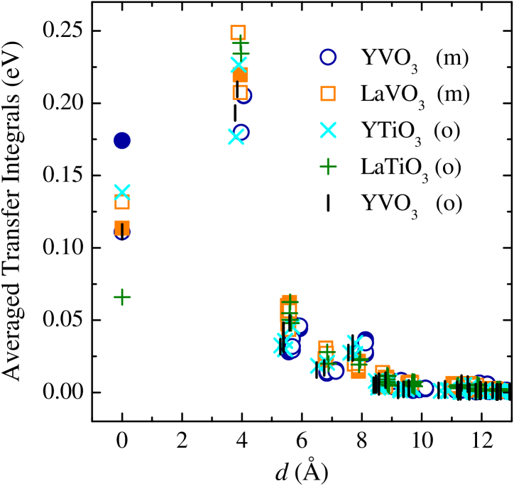
Figure 6: (Color online) Behavior of averaged parameters of the kinetic energy for various perovskite compounds. In the orthorhombic (o) structure, all four sublattices of the transition-metal sites are equivalent as they can be transformed to each other by the symmetry operations of the $D_{2h}^{16}$ group. In the monoclinic (m) structure, the transfer interactions corresponding to two different sublattices are shown by closed and open symbols. For other notations, see Fig. 5.

The next important contribution to the CF splitting comes from the nonsphericity of the Madelung potential. This effect is comparable with the CF splitting of the covalent type. We have also found that there are several different contributions to the CF splitting, which tend to cancel each other. For example, the CF splitting of the covalent type in YTiO₃ and LaTiO₃ is largely compensated by the nonsphericity of the Madelung potential coming from the region encircling the the neighboring oxygen sites and corresponding to the cut-off radius $d$$\sim$$2$ Å in Fig. 7.comment.8 The next important contribution comes from the Y/La and Ti sites, located in the next coordination spheres ($d$$\sim$$4$ Å). In some compounds, even longer-range interactions spreading up to $d$$\sim$$10$ Å can have a relatively large weight in the sum (2).

Figure 7: Convergence of the crystal-field splitting as the function of cut-off radius in Eq. (2).

The final scheme of the “$t_{2g}$”-level splitting, which takes into account all these effects, is summarized in Fig. 8.

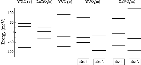
Figure 8: $t_{2g}$-level splitting in various compounds. The notations “site 1” and “site 3” correspond to two nonequivalent transition-metal sites in the monoclinic structure (shown in Fig. 2).

The splitting is not particularly large. Nevertheless, as we shall see below, it appears to be sufficient in order to explain the experimentally observed orbital ordering and the magnetic ground state in all considered compounds, except LaTiO₃. The Madelung potential changes not only the magnitude of the crystal-field splitting, but also the type of the atomic “$t_{2g}$”-orbitals, which are split off by the distortion (Table 1).

Table 1: Lowest (for YTiO₃ and LaTiO₃) and highest (for YVO₃ and LaVO₃) atomic orbital obtained from the diagonalization of the site-diagonal part of the model Hamiltonian in the downfolding method (denoted as the “covalent part”) and and after including the nonsphericity of the Madelung potential (denoted as “total”). The symbols ‘o’ and ‘m’ stand for orthorhombic and monoclinic phases, respectively. The order of the basis orbitals is ${\rm xy}$, ${\rm yz}$, ${\rm z^{2}}$, ${\rm zx}$, and ${\rm x^{2}}$$-$${\rm y^{2}}$, in the orthorhombic coordinate frame. The positions of the transition-metal sites are shown in Fig. 2.

compound	phase	site	covalent part	total
YTiO3	o	1	( $0.32$, $0.78$, $0.36$,$-$$0.33$,$-$$0.22$)	($-$$0.13$, $0.45$, $0.38$,$-$$0.61$, $0.50$)
LaTiO3	o	1	($-$$0.32$, $0.73$, $0.10$, $0.18$,$-$$0.57$)	($-$$0.06$, $0.85$, $0.15$, $0.34$, $0.37$)
YVO3	o	1	( $0.04$, $0.84$, $0.19$,$-$$0.22$, $0.47$)	( $0.29$, $0.90$, $0.25$,$-$$0.22$,$-$$0.06$)
YVO3	m	1	($-$$0.04$, $0.47$, $0.19$,$-$$0.61$, $0.60$)	( $0.12$, $0.54$, $0.18$,$-$$0.74$, $0.33$)
		3	($-$$0.01$, $0.04$,$-$$0.09$, $0.79$, $0.60$)	( $0.28$, $0.24$,$-$$0.28$, $0.89$,$-$$0.05$)
LaVO3	m	1	( $0.04$,$-$$0.31$, $0.11$, $0.80$,$-$$0.49$)	( $0.16$, $0.09$, $0.01$, $0.98$,$-$$0.04$)
		3	($-$$0.01$, $0.37$, $0.10$, $0.75$, $0.54$)	($-$$0.09$, $0.55$, $0.14$, $0.78$, $0.24$)

The type of these orbitals is extremely important in the analysis of the magnetic properties.

Finally, both magnitude and form of the CF splitting can be different for the nonequivalent transition-metal sites in the monoclinic structure. Therefore, one can generally expect rather different magnetic behavior in two nonequivalent ${\bf ab}$-planes of the monoclinic phase.

III.2 Effective Coulomb Interactions

The effective Coulomb interaction in the $t_{2g}$ band is defined as the energy cost for moving an electron between two Wannier orbitals, $\tilde{W}_{\bf R}^{\alpha}$ and $\tilde{W}_{{\bf R}^{\prime}}^{\beta}$, which have been initially populated by $\mathfrak{n}_{{\bf R}\alpha}$ and $\mathfrak{n}_{{\bf R}^{\prime}\beta}$ electrons:

$$U_{\alpha\alpha\beta\beta}=E\left[\mathfrak{n}_{{\bf R}\alpha}+1,\mathfrak{n}_{{\bf R}^{\prime}\beta}-1\right]-E\left[\mathfrak{n}_{{\bf R}\alpha},\mathfrak{n}_{{\bf R}^{\prime}\beta}\right].$$

More generally, one can consider the electron transfer from any linear combination of the Wannier orbitals at the site ${\bf R}^{\prime}$ to any linear combination at the site ${\bf R}$. This define the full matrix of screened Coulomb interactions $\hat{U}$$=$$\|U_{\alpha\beta\gamma\delta}\|$. It can be calculated under certain approximations, which have been discussed in details in Ref. condmat05, . The method consists of two parts.
1. First, we perform the standard constraint-LDA (c-LDA) calculations and artificially switch off all matrix elements of hybridization involving the atomic $3d$-states.cLDA This part takes into account the screening of Coulomb interactions caused by the relaxation of the $3d$-atomic basis functions and the redistribution of the rest of the charge density. Typical values of on-site Coulomb interactions ($u$) obtained in this approach for the Ti- and V-based perovskites vary between $8.5$ and $9.3$ eV. Using a similar approach, one can calculate the intraatomic exchange coupling constant ($j$), which is about $0.9$ eV for all considered compounds. Finally, from the obtained parameters $u$ and $j$, one can restore the full $5$$\times$$5$$\times$$5$$\times$$5$ matrix $\hat{u}$$\equiv$$\|u_{\alpha\beta\gamma\delta}\|$ of screened Coulomb interactions between atomic $3d$-orbitals with the same spin, as it is typically done in the LDA$+$$U$ method.PRB94
2. Then, we switch on the hybridization and evaluate the screening caused by the change of this hybridization between the atomic $3d$-orbitals and the rest of the basis states in the random-phase approximation (RPA):

$$\hat{U}=\left[1-\hat{u}\hat{P}(0)\right]^{-1}\hat{u}.$$ (3)

This scheme implies that different channels of screening can be included consecutively. Namely, the $\hat{u}$-matrix derived from c-LDA is used as the bare Coulomb interaction in the Dyson equation (3), and the $5$$\times$$5$$\times$$5$$\times$$5$ polarization matrix $\hat{P}$$\equiv$$\|P_{\alpha\beta\gamma\delta}\|$ describes solely the effects of hybridization of the $3d$-states with O($2p$), and either Y($4d$) or La($5d$) states, which lead to the formation of the distinct oxygen-$2p$, transition-metal $t_{2g}$, and a hybrid $e_{g}$ band in Fig. 1. The matrix elements $\hat{P}$ are given by

$$P_{\alpha\beta\gamma\delta}(\omega)=\sum_{n{\bf k}}\sum_{n^{\prime}{\bf k}^{\prime}}\frac{(\mathfrak{n}_{n{\bf k}}-\mathfrak{n}_{n^{\prime}{\bf k}^{\prime}})d^{\dagger}_{\alpha n^{\prime}{\bf k}^{\prime}}d_{\beta{n\bf k}}d^{\dagger}_{\gamma n{\bf k}}d_{\delta n^{\prime}{\bf k}^{\prime}}}{\omega-\varepsilon_{n^{\prime}{\bf k}^{\prime}}+\varepsilon_{n{\bf k}}+i\delta(\mathfrak{n}_{n{\bf k}}-\mathfrak{n}_{n^{\prime}{\bf k}^{\prime}})},$$ (4)

where $\{\varepsilon_{n{\bf k}}\}$ and $\{\mathfrak{n}_{n{\bf k}}\}$ are LDA eigenvalues and occupation numbers for the band $n$ and momentum ${\bf k}$ in the first Brillouin zone (the spin index is already included in the definition of $n$) and $d_{\gamma{n{\bf k}}}$$=$$\langle\tilde{\chi}_{\gamma}|\psi_{n{\bf k}}\rangle$ is the projection of LDA eigenstate $\psi_{n{\bf k}}$ onto the atomic $3d$ orbital $\tilde{\chi}_{\gamma}$.

Hence, we obtain a $5$$\times$$5$$\times$$5$$\times$$5$ matrix of screened Coulomb interactions in the basis of all five $3d$ orbitals. This matrix is then transformed into the local coordinate frame spanned by three “$t_{2g}$” orbitals with the same spin. The obtained $3$$\times$$3$$\times$$3$$\times$$3$ matrix is expanded in the spin subspace using the orthogonality condition between Wannier orbitals with different spins. This yields a $6$$\times$$6$$\times$$6$$\times$$6$ matrix $\hat{U}$, which is used in the actual calculations.

Only for explanatory purposes, we fit $\hat{U}$ in terms of two Kanamori parameters: the intra-orbital Coulomb interaction ${\cal U}$ and the exchange interaction ${\cal J}$.Kanamori2 The results of such fitting are shown in Table 2. There is the clear dependence of the parameter ${\cal U}$ on the local environment in solid, which is captured by the RPA calculations.condmat05 Generally, the value of ${\cal U}$ is larger for more distorted Y-compounds. There is also a clear correlation between the value of ${\cal U}$ and the magnitude of local distortion around two nonequivalent transition-metal sites in the monoclinic phases: the sites experiencing larger distortion (according to the magnitude of the CF splitting in Fig. 8) have larger ${\cal U}$. On the other hand, ${\cal J}$ is practically insensitive to the local environment in solids.

Table 2: Results of fitting of the effective Coulomb interactions in the $t_{2g}$ band obtained in the hybrid c-LDA+RPA approach in terms of two Kanamori parameters: the intra-orbital Coulomb interaction ${\cal U}$ and the exchange interaction ${\cal J}$ (in eV).Kanamori2 The symbols ‘o’ and ‘m’ stand for the orthorhombic and monoclinic phases, respectively. The positions of the transition-metal sites are shown in Fig. 2.

compound	phase	site	${\cal U}$	${\cal J}$
YTiO3	o	1	$3.45$	$0.62$
LaTiO3	o	1	$3.20$	$0.61$
YVO3	o	1	$3.27$	$0.63$
YVO3	m	1	$3.19$	$0.63$
		3	$3.26$	$0.63$
LaVO3	m	1	$3.11$	$0.62$
		3	$3.12$	$0.62$

IV Solution of Model Hamiltonian

In this section we briefly discuss the methods of solution of the model Hamiltonian (1). We start with the simplest HF approach, which totally neglect the correlation effects. Then, we consider two simple corrections to the HP approximation, which allow to include some of these effects. One is the second-order perturbation theory for the total energy. It shares common problems of the regular (nondegenerate) perturbation theory and allows to calculate easily the correction to the total energy, starting from the single-Slater-determinant HF approximation for the wavefunctions. Therefore, we expect this method to work well for the systems where the orbital degeneracy is already lifted and the ground state is described reasonably well by a single Slater determinant, so that other corrections can be treated as a perturbation. The second scheme is the variational superexchange theory for the $d^{1}$ perovskites, which takes into account the multiplet structure of the excited atomic states. It allows to study the effect of electron correlations on the orbital ordering. However, it is limited by typical approximations made in the theory of superexchange interactions, which treat all transfer integrals as a perturbation.

All calculations have been performed in the basis of Wannier functions $\{\tilde{W}_{\bf R}^{\alpha}\}$, which have a finite weight at the central transition-metal sites as well as the oxygen and other atomic sites located in the nearest neighborhood to the transition-metal atoms. In order to calculate the local quantities, associated with the transition-metal atoms, such as the spin or orbital magnetic moments as well as the distributions of the charge densities, the Wannier functions have been expanded over the standard LMTO basis, and the aforementioned quantities have been obtained by the integration over the atomic spheres of the transition-metal sites.

IV.1 Hartree-Fock Approximation

The Hartree-Fock approximation provides the simplest solution of the many-body problem described by the model Hamiltonian (1). In this case, the trial wavefunction for the many-electron ground state is searched in the form of a single Slater determinant $|S\{\varphi_{n{\bf k}}\}\rangle$, which is constructed from the one-electron orbitals $\{\varphi_{n{\bf k}}\}$. The latter are subjected to the variational principle and requested to minimize the total energy

$$E_{\rm HF}=\min_{\{\varphi_{n{\bf k}}\}}\langle S\{\varphi_{n{\bf k}}\}|\hat{\cal{H}}|S\{\varphi_{n{\bf k}}\}\rangle$$

for a given number of particles $\cal{N}$, yielding the set of well-known HF equations:

$$\left(\hat{h}_{\bf k}+\hat{V}\right)|\varphi_{n{\bf k}}\rangle=\varepsilon_{n{\bf k}}|\varphi_{n{\bf k}}\rangle,$$ (5)

where $\hat{h}_{\bf k}$$\equiv$$\|h_{\bf k}^{\alpha\beta}\|$ is the kinetic part of the model Hamiltonian (1) in the reciprocal space: $h_{\bf k}^{\alpha\beta}$$=$$\frac{1}{N}\sum_{{\bf R}^{\prime}}h^{\alpha\beta}_{{\bf R}{\bf R}^{\prime}}e^{-i{\bf k}\cdot({\bf R}-{\bf R}^{\prime})}$ ($N$ being the number of sites), and $\hat{V}$$\equiv$$\|V_{\alpha\beta}\|$ is the HF potential:

$$V_{\alpha\beta}=\sum_{\gamma\delta}\left(U_{\alpha\beta\gamma\delta}-U_{\alpha\delta\gamma\beta}\right)n_{\gamma\delta}.$$ (6)

Eq. (5) is solved self-consistently together with the equation

$$\hat{n}=\sum_{n{\bf k}}^{occ}|\varphi_{n{\bf k}}\rangle\langle\varphi_{n{\bf k}}|$$

for the density matrix $\hat{n}$$\equiv$$\|n_{\alpha\beta}\|$ in the basis of Wannier orbitals.

After the self-consistency, the total energy can be calculated as

$$E_{\rm HF}=\sum_{n{\bf k}}^{occ}\varepsilon_{n{\bf k}}-\frac{1}{2}\sum_{\alpha\beta}V_{\beta\alpha}n_{\alpha\beta}.$$

Using $\{\varepsilon_{n{\bf k}}\}$ and $\{\varphi_{n{\bf k}}\}$, one can calculate the Green function in the HF approximation:

$$\hat{\cal G}_{{\bf RR}^{\prime}}(\omega)=\sum_{n{\bf k}}\frac{|\varphi_{n{\bf k}}\rangle\langle\varphi_{n{\bf k}}|}{\omega-\varepsilon_{n{\bf k}}+i\delta}e^{i{\bf k}\cdot({\bf R}-{\bf R}^{\prime})}.$$

The latter is widely used for the analysis of interatomic magnetic interactions:JHeisenberg

$$J_{{\bf RR}^{\prime}}=\frac{1}{2\pi}{\rm Im}\int_{-\infty}^{\varepsilon_{\rm F}}d\varepsilon{\rm Tr}_{L}\left\{\hat{\cal G}_{{\bf RR}^{\prime}}^{\uparrow}(\omega)\Delta\hat{V}\hat{\cal G}_{{\bf R}^{\prime}{\bf R}}^{\downarrow}(\omega)\Delta\hat{V}\right\},$$ (7)

where $\hat{\cal G}_{{\bf RR}^{\prime}}^{\uparrow,\downarrow}$$=$$\frac{1}{2}{\rm Tr}_{S}\{(\hat{1}$$\pm$$\hat{\sigma}_{z})\hat{\cal G}_{{\bf RR}^{\prime}}\}$ is the projection of the Green function onto the majority ($\uparrow$) and minority ($\downarrow$) spin states, $\Delta\hat{V}$$=$${\rm Tr}_{S}\{\hat{\sigma}_{z}\hat{V}\}$ is the magnetic (spin) part of the HF potential, ${\rm Tr}_{S}$ (${\rm Tr}_{L}$) denotes the trace over the spin (orbital) indices, $\hat{1}$ and $\hat{\sigma}_{z}$ are correspondingly unity and Pauli matrices of the dimension $6$, and $\varepsilon_{\rm F}$ is the Fermi energy.

The interatomic magnetic interactions $\{J_{{\bf RR}^{\prime}}\}$ characterize the spin stiffness of the magnetic phase. Therefore, they can be directly compared with the experimental spin-wave spectra derived from the inelastic neutron scattering measurement.

According to Eq. 7, $J_{{\bf RR}^{\prime}}$$>$$0$ ($<$$0$) means that for a given magnetic structure, the spin arrangement in the bond $\langle{\bf RR}^{\prime}\rangle$ corresponds to the local minimum (maximum) of the total energy. However, in the following we will use the universal notations, according to which $J_{{\bf RR}^{\prime}}$$>$$0$ and $<$$0$ will stand the ferromagnetic and antiferromagnetic coupling, respectively. This corresponds to the local mapping onto the Heisenberg model of the form

$$E_{\rm Heis}=-\sum_{\langle{\bf RR}^{\prime}\rangle}J_{{\bf RR}^{\prime}}{\bf e}_{\bf R}\cdot{\bf e}_{{\bf R}^{\prime}},$$ (8)

where ${\bf e}_{\bf R}$ is the direction of the spin magnetic moment at the site ${\bf R}$. The “local mapping” means that, strictly speaking, Eq. 8 is justified only for the infinitesimal rotations of the spin magnetic moment near an equilibrium.

The magnetic interactions are extremely sensitive to the orbital ordering. Therefore, they can be regarded as the local prob of the orbital ordering in each magnetic state.

IV.2 Second Order Perturbation Theory for Correlation Energy

The simplest way to go beyond the HF approximation is to include the correlation interactions in the second order of perturbation theory for the total energy.cor2ndorder The correlation interaction (or a fluctuation) is defined as the difference between true many-body Hamiltonian (1), and its one-electron counterpart, obtained at the level of HF approximation:

$$\hat{\cal{H}}_{\rm C}=\sum_{\bf R}\left(\frac{1}{2}\sum_{\alpha\beta\gamma\delta}U_{\alpha\beta\gamma\delta}\hat{c}^{\dagger}_{{\bf R}\alpha}\hat{c}^{\dagger}_{{\bf R}\gamma}\hat{c}^{\phantom{\dagger}}_{{\bf R}\beta}\hat{c}^{\phantom{\dagger}}_{{\bf R}\delta}-\sum_{\alpha\beta}V_{\alpha\beta}\hat{c}^{\dagger}_{{\bf R}\alpha}\hat{c}^{\phantom{\dagger}}_{{\bf R}\beta}\right).$$ (9)

By treating $\hat{\cal{H}}_{\rm C}$ as a perturbation, the correlation energy can be easily estimated as:cor2ndorder

$$E_{\rm C}=-\sum_{S}\frac{\langle G|\hat{\cal{H}}_{\rm C}|S\rangle\langle S|\hat{\cal{H}}_{\rm C}|G\rangle}{E_{\rm HF}(S)-E_{\rm HF}(G)},$$ (10)

where $|G\rangle$ and $|S\rangle$ are the Slater determinants corresponding to the low-energy ground state in the HF approximation, and the excited state, respectively. Due to the variational properties of the Hartree-Fock approach, the only processes which contribute to $E_{\rm C}$ correspond to the two-particle excitations, for which each $|S\rangle$ is obtained from $|G\rangle$ by replacing two one-electron orbitals, say $\varphi_{n_{1}{\bf k}_{1}}$ and $\varphi_{n_{2}{\bf k}_{2}}$, from the occupied part of the spectrum by two unoccupied orbitals, say $\varphi_{n_{3}{\bf k}_{3}}$ and $\varphi_{n_{4}{\bf k}_{4}}$. Hence, using the notations of Sec. III, the matrix elements take the form:

$$\langle S|\hat{\cal{H}}_{\rm C}|G\rangle=\langle\varphi_{n_{3}{\bf k}_{3}}\varphi_{n_{4}{\bf k}_{4}}|v_{\rm scr}|\varphi_{n_{1}{\bf k}_{1}}\varphi_{n_{2}{\bf k}_{2}}\rangle-\langle\varphi_{n_{3}{\bf k}_{3}}\varphi_{n_{4}{\bf k}_{4}}|v_{\rm scr}|\varphi_{n_{2}{\bf k}_{2}}\varphi_{n_{1}{\bf k}_{1}}\rangle.$$ (11)

These matrix elements satisfy the following condition: $\langle S|\hat{\cal{H}}_{\rm C}|G\rangle$$\sim$$\frac{1}{N}\sum_{\bf R}e^{i({\bf k}_{3}+{\bf k}_{4}-{\bf k}_{1}-{\bf k}_{2})\cdot{\bf R}}$, provided that the screened Coulomb interactions are diagonal with respect to the site indices. In the following we will retain only the ${\bf R}$$=$$0$ part in this sum. This corresponds to the single-site approximation for the correlation interactions, which is known to be good for three-dimensional systems and becomes exact in the limit of infinite spacial dimensions.DMFT

Finally, we employ a common approximation of noninteracting quasiparticles and replace the denominator of Eq. (10) by the linear combination of HF eigenvalues: $E_{\rm HF}(S)$$-$$E_{\rm HF}(G)$$\approx$$\varepsilon_{n_{3}{\bf k}_{3}}$$+$$\varepsilon_{n_{4}{\bf k}_{4}}$$-$$\varepsilon_{n_{1}{\bf k}_{1}}$$-$$\varepsilon_{n_{2}{\bf k}_{2}}$.cor2ndorder

The form of Eq. (10) implies that the HF ground state is nondegenerate, and the correlation effects can be systematically included by considering the regular perturbation theory expansion. It does not apply to the cubic systems, where the ground state is infinitely degenerate (with respect to different orbital configurations), and where a suitable approach for the correlation energy should be based on the degenerate perturbation theory.KhaliullinMaekawa Thus, the use of Eq. (10) implies that the orbital degeneracy is already lifted by the crystal distortion. As we shall see below, this approximation can be justified for a number of systems.

IV.3 Effects of Multiplet Structure in the Theory of Superexchange Interactions

Another method, which allows to treat some correlation effects beyond the mean-field HF approximation is based on the generalization of the theory of superexchange interactions in order to describe the correct multiplet structure of the atomic states. Similar idea has been discussed in the context of colossal magnetoresistive perovskite manganites.SEmultiplet The formulation is extremely simple for the $d^{1}$ compounds, like YTiO₃ and LaTiO₃.

The superexchange interaction in the bond $\langle{\bf RR}^{\prime}\rangle$ is basically the gain of the kinetic energy, which is acquired by an electron occupying the atomic orbital $\phi_{\bf R}$ of site ${\bf R}$ in the process of virtual hoppings into the subspace of unoccupied orbitals of the (neighboring) site ${\bf R}^{\prime}$, and vice versa.PWA ; KugelKhomskii In the atomic limit for the $d^{1}$ compounds, there is only one $t_{2g}$ electron at each Ti site. This is essentially an one-electron problem, where the form of the atomic orbital $\phi_{\bf R}$ is determined by the site-diagonal part of kinetic-energy $\|h_{\bf RR}^{\alpha\beta}\|$, incorporating the effects of the spin-orbit interaction and the CF splitting. Therefore, in the pure atomic limit, the ground-state wavefunction for each bond $\langle{\bf RR}^{\prime}\rangle$ can be described by a single Slater determinant:

$$|G_{{\bf RR}^{\prime}}\rangle=\frac{1}{\sqrt{2}}\left\{\phi_{\bf R}(1)\phi_{{\bf R}^{\prime}}(2)-\phi_{{\bf R}^{\prime}}(1)\phi_{\bf R}(2)\right\}.$$

Then, $\phi_{\bf R}$ and $\phi_{{\bf R}^{\prime}}$ are expanded over the Wannier orbitals associated with the site ${\bf R}$ and ${\bf R}^{\prime}$ and the transfer integrals connecting different Wannier orbitals are treated as a perturbation. The excited states at the sites ${\bf R}$ and ${\bf R}^{\prime}$, which appear in the process of the virtual hoppings are the two-electron states and subjected to the multiplet splitting. This is exactly the point where the electron correlations, beyond the HF approximation, enter the problem. In order to incorporate these effects we note that from $m$$=$$6$ Wannier spin-orbitals $\{\tilde{W}_{\bf R}^{\alpha}\}$ at each Ti site, one can construct $\frac{1}{2}m(m$$-$$1)$$=$$15$ antisymmetric two-electron Slater’s determinants $\{|S\rangle\}$ ($S$$=$$1,$$\dots,$$15$), which can be used as the basis for the screened Coulomb interactions in the excited state: $U_{SS^{\prime}}$$=$$\langle S|v_{\rm scr}|S^{\prime}\rangle$. The diagonalization of this $15$$\times$$15$ matrix yield the complete set of eigenvalues $\{E_{{\bf R}M}\}$ and eigenfunctions $\{|{\bf R}M\rangle\}$ of the two-electron states at the site ${\bf R}$ ($M$$=$$1,$$\dots,$$15$). An example of such a multiplet structure for YTiO₃ and LaTiO₃ is shown in Fig. 9.

Figure 9: The multiplet structure of the excited atomic configuration $t_{2g}^{2}$ in YTiO₃ and LaTiO₃.

According to the first Hund rule, the lowest-energy configuration corresponds to the spin-triplet state ${\rm{}^{3}T_{1g}}$. The degeneracy of the ${\rm{}^{3}T_{1g}}$, ${\rm{}^{1}E_{g}}$, and ${\rm{}^{3}T_{2g}}$ levels is lifted by the orthorhombic distortion, which affects the matrix elements of the effective $\hat{U}$ via the RPA channel of screening. The splitting is larger for the more distorted YTiO₃.

In order to calculate the energy gain caused by the superexchange interactions, the eigenfunctions $\{|{\bf R}M\rangle\}$ shall be projected onto the physical subspace of two-electron states which can be created by transferring an electron from the neighboring sites. The corresponding projector operators have the form: ${\hat{\cal P}}_{\bf R}$$=$$\sum_{\alpha}|P_{\bf R}^{\alpha}\rangle\langle P_{\bf R}^{\alpha}|$, where $|P_{\bf R}^{\alpha}\rangle$$=$$\frac{1}{\sqrt{2}}\{\phi_{\bf R}(1)\tilde{W}_{\bf R}^{\alpha}(2)$$-$$\tilde{W}_{\bf R}^{\alpha}(1)\phi_{\bf R}(2)\}$ is the Slater determinant constructed from the occupied orbital $\phi_{\bf R}$ and one of the basis Wannier orbitals $\tilde{W}_{\bf R}^{\alpha}$. In the other words, the projection ${\hat{\cal P}}_{\bf R}$ imposes an additional constraint, which guarantees that one of the orbitals in the two-electron state is $\phi_{\bf R}$. Then, the energy gain caused by the virtual hoppings in the bond $\langle{\bf RR}^{\prime}\rangle$ is given by

$$\Delta E_{{\bf RR}^{\prime}}=-\left\langle G_{{\bf RR}^{\prime}}\left|\hat{h}_{{\bf RR}^{\prime}}\left(\sum_{M}\frac{{\hat{\cal P}}_{{\bf R}^{\prime}}|{\bf R}^{\prime}M\rangle\langle{\bf R}^{\prime}M|{\hat{\cal P}}_{{\bf R}^{\prime}}}{E_{{\bf R}^{\prime}M}}\right)\hat{h}_{{\bf R}^{\prime}{\bf R}}+({\bf i}\leftrightarrow{\bf j})\right|G_{{\bf RR}^{\prime}}\right\rangle.$$ (12)

The total energy of the system in the superexchange approximation is obtained after summation over all bonds, which should be combined with the site-diagonal elements, incorporating the effects of the CF splitting and the relativistic spin-orbit interaction:

$$E_{\rm SE}=\sum_{\bf R}\langle\phi_{\bf R}|\hat{h}_{\bf RR}|\phi_{\bf R}\rangle+\sum_{\langle{\bf RR}^{\prime}\rangle}\Delta E_{{\bf RR}^{\prime}}.$$

Finally, the set of occupied orbitals $\{\phi_{\bf R}\}$ is obtained by minimizing $E_{\rm SE}$, e.g., using the steepest descent method.

For a given orbital ordering, the multiplet effects are expected to be more important in the case of the AFM spin ordering, where an electron comes to the neighboring site with the opposite direction of spin. In this case, the excited configuration is subjected to the multiplet splitting into the spin-singlet and spin-triplet states, which additionally stabilizes the AFM spin state.comment.5

V Results and Discussions

In this section we present results of solution the model Hamiltonian (1) for the distorted perovskite compounds. We start with Y-based perovskites, where the orbital ordering is largely controlled by the CF splitting coming from the experimental lattice distortion. We will show that this distortion imposes a severe constraint on the magnetic properties and predetermines the type of the magnetic ground state. Then, we turn to the La-based perovskites, where the situation is less clear: while the magnetic structure of LaVO₃ can be still understood on the basis of its experimental lattice structure, LaTiO₃ poses many open and unresolved questions.

First, we will consider the impact of the crystal structure without the spin-orbit interaction. The effects of the spin-orbit interaction will be discussed separately in Sec. V.5.

V.1 YVO₃

YVO₃ exhibits two structural phase transitions.Blake ; Tsvetkov The first one is the second-order transition from orthorhombic ($D_{2h}^{16}$) to monoclinic (apparently $D_{2h}^{5}$) phase, which takes places at $200$ K and is believed to coincide with the onset of the orbital ordering. The second one is the first-order transition at $77$ K from monoclinic to another orthorhombic phase. The magnetic transition temperature is $116$ K, which lies in the monoclinic region and does not coincide with any structural phase transition. On the other hand, the change of the crystal structure at $77$ K coincides with the magnetic phase transition. The magnetic structure in the interval $77$ K $<$ T $<$ $116$ K is C-type AFM, while below $77$ K it becomes G-type AFM.

V.1.1 Low-temperature orthorhombic phase $({\rm T<77~{}K})$

YVO₃ has the largest CF splitting amongst perovskite compounds, which crystallize in the orthorhombic phase (Fig. 8). It lowers the energies of two $t_{2g}$ levels – just enough to accommodate two $d$ electrons. The highest level is separated from the middle one by a $111$ meV gap. Therefore, the orbital ordering in this $d^{2}$ compound is expected to be quenched (at least partially) by the crystal distortion.

This is clearly seen in our Hartree-Fock calculations. The orbital ordering depends on the magnetic state. However, this dependence is weak and can be hardly seen on the plot (Fig. 10).

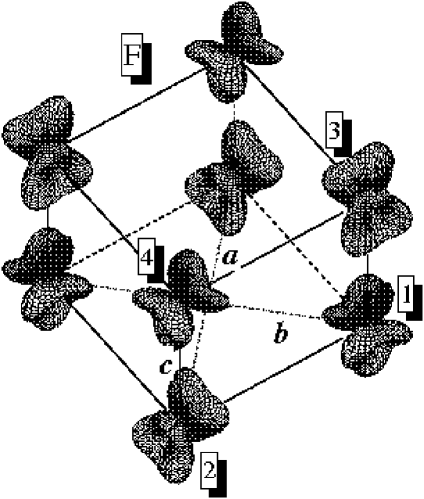
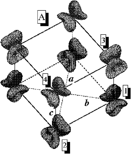
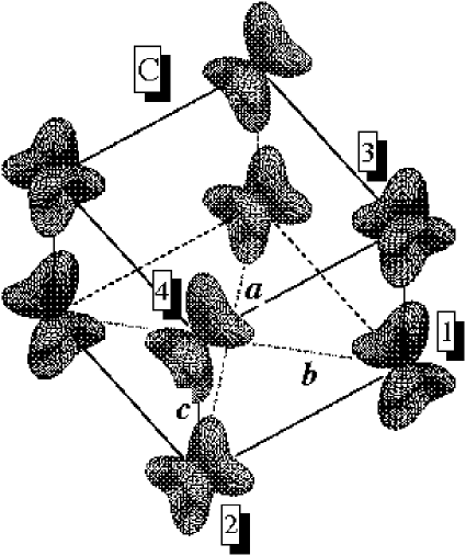
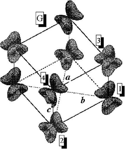
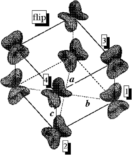
Figure 10: (Color online) Distribution of the charge density around V-sites in various magnetic phases of orthorhombically distorted YVO₃ (${\rm T}$$<$$77$ K), as obtained in Hartree-Fock calculations. Different magnetic sublattices are shown by different colors.

The form of the orbital ordering, which can be schematically viewed as an alternation of the ($xy$,$yz$) and ($xy$,$zx$) orbitals in the cubic coordinate frame associated with the VO₆ octahedra, is in an excellent agreement with the theoretical prediction of Sawada and Terakura based on the semi-empirical LDA$+$$U$ method,SawadaTerakura which was later on confirmed by the synchrotron x-ray-diffraction measurement.Noguchi

The first important question, which we would like to address here is where does this orbital ordering come from? In Fig. 11 we show results of calculations obtained using three different settings for the site-diagonal part of kinetic-energy part of the model Hamiltonian: (i) $h_{\bf RR}^{\alpha\beta}$$=$$0$ (no CF splitting); (ii) the parameters $\{h_{\bf RR}^{\alpha\beta}\}$ extracted from the downfolding method, which takes into account only the covalent type of the CF splitting; and (iii) the parameters $\{h_{\bf RR}^{\alpha\beta}\}$ obtained in the downfolding method and corrected for the nonsphericity of the Madelung potential (2).

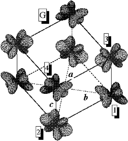
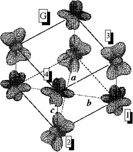
Figure 11: (Color online) Orbital ordering in the G-type antiferromagnetic phase of orthorhombically distorted YVO₃ computed without crystal field (left), including the crystal field of the covalent type (center), and the crystal field of both covalent and Madelung types (right).

One can clearly see that in order to reproduce the correct orbital ordering, all contributions to the CF splitting appear to be important. Had we neglected some of these contributions, not only the orbital ordering but also the magnetic ground state would have been different. For example, without the Madelung term, the magnetic ground state is expected to be of the A-type, in clear disagreement with the experimental data.

As it has been already discussed by other authors,SawadaTerakura ; MizokawaFujimori ; FangNagaosa the C-type orbital ordering shown in Fig. 10 favors the G-type AFM spin ordering, which emerges as the ground state already at the level of HF calculations (Table 3). The order of the magnetic states, corresponding to the increase of the total energy, is G$\rightarrow$C$\rightarrow$flip$\rightarrow$A$\rightarrow$F, which is well consistent with results of all-electron LDA$+$$U$ calculations.SawadaTerakura ; FangNagaosa ; comment.3

Table 3: Magnetic interactions ($J_{{\bf RR}^{\prime}}$), Hartree-Fock energies ($E_{\rm HF}$), and total energies ($E_{\rm tot}$) in the orthorhombic phase of YVO₃ (${\rm T}$$<$$77$ K). The energies are measured from the most stable magnetic state in meV per one formula unit. The magnetic interactions are measured in meV. The total energy is defined as Hartree-Fock energy plus correlation energies ($E_{\rm C}$) in the second order of perturbation theory: $E_{\rm tot}$$=$$E_{\rm HF}$$+$$E_{\rm C}$.

phase	$J_{12}$	$J_{13}$	$J_{24}$	$J_{34}$	$E_{\rm HF}$	$E_{\rm tot}$
F	$-$$1.4$	$-$$3.6$	$-$$3.6$	$-$$1.4$	$21.7$	$27.1$
A	$-$$2.5$	$-$$3.7$	$-$$3.7$	$-$$2.5$	$14.6$	$17.3$
C	$-$$4.7$	$-$$4.9$	$-$$4.9$	$-$$4.7$	$10.1$	$11.7$
G	$-$$4.4$	$-$$4.8$	$-$$4.8$	$-$$4.4$	$0$	$0$
flip	$-$$4.0$	$-$$4.8$	$-$$3.9$	$-$$1.8$	$11.6$	$14.0$

However, the orbital ordering is not fully quenched by the crystal distortion and to certain extent can adjust the change of the magnetic state through the Kugel-Khomskii mechanism.KugelKhomskii This is seen particularly well in the behavior of interatomic magnetic interactions, which reveal an appreciable dependence on the magnetic state. For example, by going from the G-state to the F-state, the in-plane interaction $J_{12}$ ($J_{34}$) changes by nearly 70%, and the inter-plane interaction $J_{13}$ ($J_{24}$) changes by 25%.

In agreement with the experimental finding,Ulrich2003 ) the magnetic interactions in the G-type AFM ground state are nearly isotropic. However, this isotropic behavior can be easily destroyed by a small change of the orbital ordering, which is realized for example in other magnetic states.

The absolute values of $J_{12}$ and $J_{13}$ obtained in the HF calculations for the G-type AFM phase are underestimated by about $1$ meV in comparison with the experimental parameters extracted from the fit of the spin-wave spectra ($J_{12}$$=$$J_{13}$$=-$$5.7$$\pm$$0.3$ meV). This seems to be reasonable because the HF method is a single-Slater-determinant approach, which does not include the correlation effects. The magnitude of the correlations energy depends on the magnetic state and is expected to be larger in the case of the AFM spin alignment, where the net magnetization is zero and the choice of the many-electron wave function in the form of a single Slater determinant is always an approximation.Imai On the other hand, the saturated ferromagnetic state can be described relatively well by a single Slater determinant. All these trends are clearly seen in the total energy calculations, which take into account the correlation effect in the second order of perturbation theory (Table 3). The correlations additionally stabilize the G-type AFM ground state relative to other magnetic states. However, it does not change the order of the magnetic states.

Unfortunately, it is not possible to estimates the effects of correlations on the interatomic magnetic interactions directly, using Eq. (7). Nevertheless, one can try to use the total energy differences between different magnetic states and map them onto the Heisenberg model.comment.4 This is a cruder approximation, which implies that the orbital ordering is completely quenched by the crystal distortion and does not depend on the magnetic state. We will use it here only in order to get a qualitative idea about the impact of correlation effects on the interatomic magnetic interactions. Then, the standard HF approximation yields $J_{12}$$=-$$3.3$ meV and $J_{13}$$=-$$4.3$ meV, the second order perturbation theory for the correlation energy yields $J_{12}$$=-$$4.1$ meV and $J_{13}$$=-$$5.4$ meV. Therefore, the $1$ meV difference between parameters of magnetic interactions obtained in the HF calculations and the experimental spin-wave dispersion data can be naturally attributed to the correlation effects. This example also clearly shows at the importance of more rigorous treatment of the correlation effects and necessity to go beyond the single-Slater-determinant HF approximation for the $t_{2g}$ perovskite oxides.

V.1.2 High-temperature monoclinic phase $({\rm 77~{}K<T<116~{}K)}$

The monoclinic distortion creates two inequivalent types of V-sites, which lie in different ${\bf ab}$-planes: (1,2) and (3,4) in Fig. 2. This leads to the new scheme of the $t_{2g}$-level splitting (Fig. 8). Energetically, the new scheme is rather similar to the previous one, observed in the orthorhombic phase. In both planes it lowers the energies of two $t_{2g}$ levels. The energy gap, which separates the highest level from the middle one is $101$ and $128$ meV for the sites 1 and 3, respectively. However, the type of the orbitals which are split off by the distortion is different (Table 1). This leads to the new type of stacking between the planes, which reminiscent the G-type orbital ordering.

However, the orbital ordering is not completely quenched by the crystal distortion and there is a substantial variation of the orbital structure depending on the magnetic state, which can be seen already in the distribution of the charge density in Fig. 12.

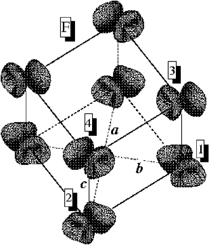
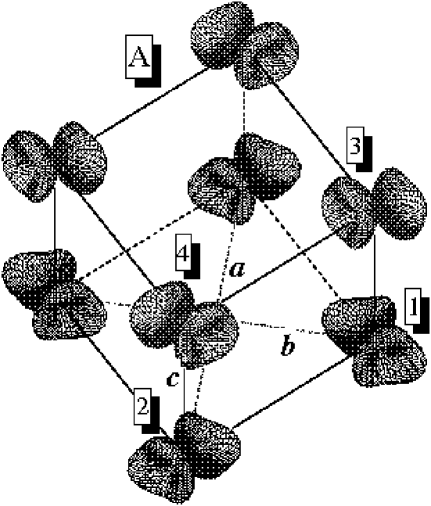
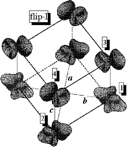
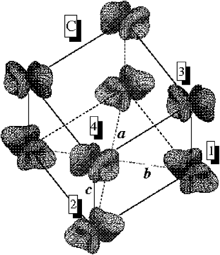
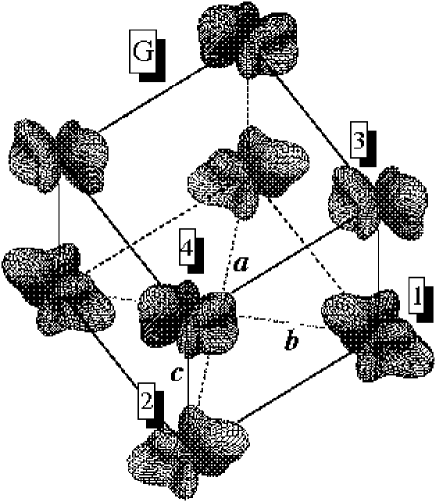
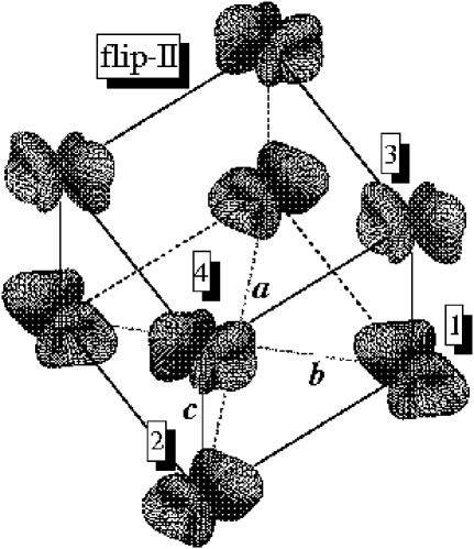
Figure 12: (Color online) Distribution of the charge density around V-sites in various magnetic phases of monoclinically distorted YVO₃, as obtained in Hartree-Fock calculations. Different magnetic sublattices are shown by different colors.

Nevertheless, the basic G-type orbital ordering pattern is clearly seen in all magnetic structures. This appears to be sufficient to stabilize the experimentally observed C-type AFM phase, which becomes the ground state already in the HF approach (Table 4). The correlation effects play a very important role. They additionally stabilize the C-type AFM ground state and reverse the order of other magnetic states (e.g., F and A in Table 4).

Table 4: Magnetic interactions ($J_{{\bf RR}^{\prime}}$), Hartree-Fock energies ($E_{\rm HF}$), and total energies ($E_{\rm tot}$) in the monoclinic phase of YVO₃ ($77$ K $<{\rm T}<$ $116$ K). See Table 3 for other notations.

phase	$J_{12}$	$J_{13}$	$J_{24}$	$J_{34}$	$E_{\rm HF}$	$E_{\rm tot}$
F	$0.1$	$2.7$	$2.7$	$-$$3.5$	$11.7$	$17.5$
A	$-$$0.3$	$2.5$	$2.5$	$-$$3.4$	$14.0$	$17.1$
C	$-$$0.9$	$2.2$	$2.2$	$-$$4.5$	$0$	$0$
G	$-$$1.6$	$1.8$	$1.8$	$-$$4.8$	$\phantom{1}6.6$	$\phantom{1}7.2$
flip-I	$-$$1.8$	$1.6$	$2.5$	$-$$3.4$	$11.5$	$14.2$
flip-II	$-$$0.4$	$2.3$	$2.8$	$-$$4.8$	$\phantom{1}4.4$	$\phantom{1}6.5$

The orbital ordering in the plane (3,4) clearly reminiscent the one observed in the orthorhombic phase (Fig. 10). The shape of orbitals in the plane (1,2) appears to be more distorted.

The behavior of interatomic magnetic interactions in the high-temperature phase of YVO₃ has attracted a considerable attention recently. The experimental spin-wave spectrum shows a clear splitting into acoustic and optical branches, which are separated by a 5 meV gap in the middle, ${\bf q}_{m}$$=$$(0,0,\pi/2c)$, point of the first Brillouin zone along the [001] direction.Ulrich2003 The splitting has been initially attributed to the dimerization effect associated with an orbital Peierls state, which should lead to the alternation of the strong and weak ferromagnetic bonds along the ${\bf c}$ axis.Ulrich2003 However, more recently the puzzling features of the experimental spectra have be naturally explained by the difference of the exchange coupling constants in the adjacent ${\bf ab}$-planes, which is expected for the monoclinic $C^{5}_{2h}$ symmetry.FangNagaosa This effect is clearly seen in our HF calculations: while the AFM exchange coupling in the plane (3,4) does not change so much in comparison with the orthorhombic phase, the one in the plane (1,2) drops by almost $4$ meV (referring to the C-type AFM state in Table 4). The value of the gap in the point ${\bf q}_{m}$ can be estimated in the linear spin-wave theory as $\Delta_{\rm SW}$$=$$2J_{13}|\sqrt{1-4J_{12}/J_{13}}$$-$$\sqrt{1-4J_{34}/J_{13}}|$. Then, using results of HF calculations we obtain $\Delta_{\rm SW}$$\approx$$6.2$ meV, which is in fair agreement with the experimental finding. We can further speculate that the ferromagnetic coupling $J_{13}$ is overestimated in the HF approximation due to the lack of the correlations effects (in the next section we shall see that this is indeed the case for the totally ferromagnetic YTiO₃). Therefore, the correlation effects will probably yield a smaller value of $\Delta_{\rm SW}$, which is proportional to $J_{13}$.

V.2 YTiO₃

YTiO₃ is a $d^{1}$ compound. The lattice distortion splits off one $t_{2g}$-level to the low-energy part of the spectrum (Fig. 8). This is just enough for trapping one $d$ electron at each Ti-site. Therefore, the situation is similar to YVO₃. The lowest $t_{2g}$-level is separated from the middle one by a 109 meV gap, which is comparable with the magnitude of the CF splitting in YVO₃.

The lattice distortion stabilizes the orbital ordering, which is shown in Fig. 13. In this case, the orbital ordering is strongly quenched by the distortion and not only the charge density but also the parameters of the magnetic interactions (Table 5), which are sensitive to the orbital ordering, only weakly depend on the magnetic state.

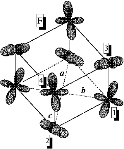
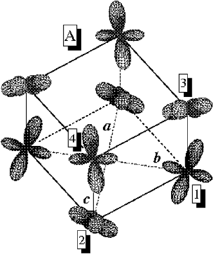
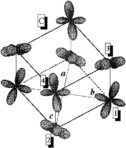
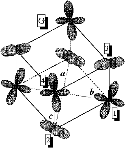
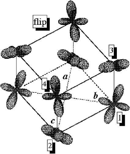
Figure 13: (Color online) Distribution of the charge density around Ti-sites in various magnetic phases of YTiO₃, as obtained in Hartree-Fock calculations. Different magnetic sublattices are shown by different colors.

Table 5: Magnetic interactions ($J_{{\bf RR}^{\prime}}$), Hartree-Fock energies ($E_{\rm HF}$), total energies ($E_{\rm tot}$), and superexchange energies ($E_{\rm SE}$) in YTiO₃. $E_{\rm SE}$ is defined as the total energy in the superexchange approximation. Other definitions are explained in Table 3.

phase	$J_{12}$	$J_{13}$	$J_{24}$	$J_{34}$	$E_{\rm HF}$	$E_{\rm tot}$	$E_{\rm SE}$
F	$3.9$	$1.2$	$1.2$	$3.9$	$0$	$0$	$0$
A	$3.9$	$1.1$	$1.1$	$3.9$	$\phantom{1}2.0$	$\phantom{1}0.8$	$\phantom{1}0.1$
C	$3.2$	$1.1$	$1.1$	$3.2$	$14.4$	$10.9$	$12.1$
G	$3.2$	$1.0$	$1.0$	$3.2$	$16.2$	$12.5$	$13.9$
flip	$3.2$	$1.1$	$1.1$	$3.9$	$\phantom{1}8.2$	$\phantom{1}6.1$	$\phantom{1}6.7$

Partly, this is because YTiO₃ has the largest on-site Coulomb interaction ${\cal U}$ amongst considered perovskite oxides (Table 2). Therefore, the superexchange contribution to the orbital ordering is expected to be smaller in comparison with the CF splitting. The obtained orbital ordering is in the excellent agreement with results of LDA$+$$U$ calculations by Sawada and Terakura,SawadaTerakura and the experimental measurement using the nuclear magnetic resonance (Ref. Itoh, ), the polarized neutron diffraction (Ref. Akimitsu, ), and the soft x-ray linear dichroism (Ref. Iga, ).

The observed orbital ordering patter is compatible with the ferromagnetic ground state, which easily emerges at the level of HF theories.SawadaTerakura ; MizokawaFujimori The same trend is clearly seen in our calculations, and both the order F$\rightarrow$A$\rightarrow$C$\rightarrow$flip$\rightarrow$G and the total-energies difference between different magnetic states obtained in the HF approximation are well consistent with the LDA$+$$U$ results of Sawada and Terakura.SawadaTerakura

The correlation effects are important. Similar to YVO₃, they tend to additionally stabilize the AFM configurations and destabilize the ferromagnetic ground state. The situation is very fragile, and after taking into account the correlation effects, the energy difference between F state and the next A-type AFM state becomes only $0.1$-$0.8$ meV per one formula unit. For the $d^{1}$ compounds, we can apply two independent schemes for studying the correlation effects: one is the second order perturbation theory and the other one is the theory of superexchange interactions, which takes into account the multiplet structure of the excited states. For YTiO₃, both scheme yields very consistent results, apart from the small quantitative difference, which is inevitable for two different approximations.

Yet, the magnetic behavior of YTiO₃ poses several open questions, which are not fully understood.

First of all, YTiO₃ is an exceptional example amongst $t_{2g}$ perovskite oxides, because the ferromagnetic ground state can be anticipated already on the basis of the canonical Goodenough-Kanamori-Anderson rules for the superexchange interactions in the simple cubic structure. This immediately revives the idea of Kugel and Khomskii about the superexchange-driven orbital ordering and the concomitant Jahn-Teller distortion, which was intensively discussed in the context of KCuF₃.KugelKhomskii Then, one may ask whether the experimental orbital ordering in YTiO₃ can be stabilized by the pure superexchange mechanism, without appealing to the CF splitting. This can be easily checked by substituting $h_{\bf RR}^{\alpha\beta}$$=$$0$ into kinetic-energy part of the model Hamiltonian. Surprisingly, the orbital ordering in the ferromagnetic state is practically the same with and without the CF splitting (Ref. 14).

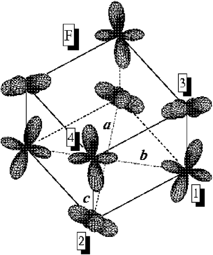
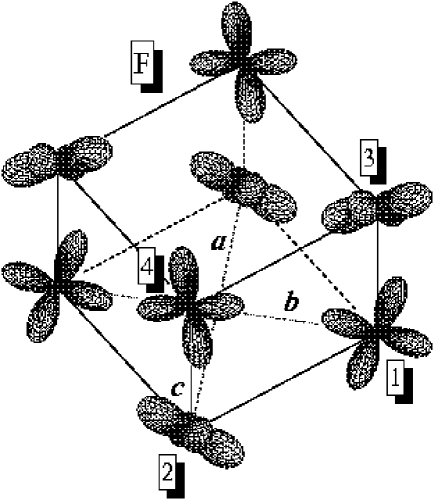
Figure 14: (Color online) Orbital ordering in the ferromagnetic phase of YTiO₃ computed with (left) and without (right) crystal-field splitting.

The interatomic magnetic interactions, $J_{12}$$=$$4.3$ meV and $J_{13}$$=$$1.6$ meV, are also consistent with the data listed in Table 5, and which include the effects of the CF splitting. This naturally explain results of our previous work (Ref.PRB04, ), where similar orbital ordering and interatomic magnetic interactions have been obtained without the Madelung term in the CF splitting. Therefore, it is tempting to conclude that the orbital ordering in YTiO₃ is driven by the superexchange interactions, and the lattice distortion simply follows the anisotropic distribution of the charge density associated with this orbital state. However, the situation is not so simple, because our calculations have been performed in the room temperature structure (T$=$$293$ K, Ref. Maclean, ), which is much higher than the Curie temperature (T_C$\approx$$30$ K, Ref. Akimitsu, ). Furthermore, the orbital ordering shown in Fig. 14 in the absence of the CF splitting takes places only in the ferromagnetic phase: had we changed the magnetic state, our orbital ordering would have been also different. Therefore, a more plausible scenario for YTiO₃ is that the lattice distortion goes first and sets up a particular form of the CF splitting, which stabilizes the experimental orbital ordering pattern and the ferromagnetic ground state. Nevertheless, the good agreement between two orbital states shown in Fig. 14 is really curious. Is it a simple coincidence or there is some physical meaning behind this result? We would like to emphasize again that the situation is totally different from YVO₃ shown in Fig. 11.

Another group of questions is related with the behavior of interatomic magnetic interactions. The first puzzling feature is the nearly isotropic experimental spin-wave spectrum reported by Ulrich et al,Ulrich2002 which cannot be explained in terms interatomic magnetic interactions derived from the first-principles electronic structure calculations. For example, the exchange parameters listed in Table 5 are clearly anisotropic, and the interactions along the ${\bf c}$-axis are much weaker than in the ${\bf ab}$-plane. A similar conclusion is expected from the analysis of the total-energy differences reported by Sawada and Terakura.SawadaTerakura Since the anisotropy of magnetic interactions is directly related with the particular form of the orbital ordering, it seems that the inelastic neutron-scattering data by Ulrich et al. are in an apparent disagreement not only with the results of the first-principles electronic structure calculations but also with a number of other experimental data, which report the same type of the orbital ordering.Itoh ; Akimitsu ; Iga Therefore, what is so special about the inelastic neutron-scattering measurements and why different experimental methods probing the orbital state yield qualitatively different conclusions in the case of YTiO₃?

The behavior of interatomic magnetic interactions predetermines not only in the form of the spin-wave spectrum, but also in the absolute value of T_C. If the magnetic properties of YTiO₃ are indeed controlled by the large lattice distortion, which is set up far above T_C, it should to be a good Heisenberg ferromagnet. This is directly seen in our HF calculations, where the parameters of interatomic magnetic interactions practically do not depend on the magnetic state (Table 5). Then, the applicability of the Heisenberg model is no longer restricted by infinitesimal rotations of the spin magnetic moments, and T_C can be easily evaluated using the standard expressions, which are well known from the theory of Heisenberg magnets.Nagaev The simplest one is the mean-field formula: $3k_{\rm B}{\rm T_{C}^{MF}}$$=$$4J_{12}$$+$$2J_{13}$, where the prefactor $S(S$$+$$1)$ is already included in the definition of our exchange parameters, although with some approximations for the spin $1/2$.comment.1 By combining this expression with the HF approximation for the exchange interactions, one finds ${\rm T_{C}^{MF}}$$=$$64$ K, which exceeds the experimental value by factor two. However, ${\rm T_{C}^{MF}}$ does not include spontaneous fluctuations and correlations between the motion of the neighboring spins. This is exactly the point where the anisotropy of exchange interactions can help to reduce the theoretical value of ${\rm T_{C}}$. Indeed, according to the Mermin-Wagner theorem,MerminWagner the two-dimensional Heisenberg model does not support any long-range spin order at any nonzero temperature. Therefore, since for $J_{13}/J_{12}$$\ll$$1$ the system will eventually approach the two-dimensional limit, it is reasonable to expect a substantial reduction of ${\rm T_{C}}$. In order to describe these effects quantitatively, one can use the spherical approximation for the Heisenberg model,Nagaev according to which $3k_{\rm B}{\rm T_{C}}$$=$$1/[\sum_{\bf k}(J_{0}$$-$$J_{\bf k})^{-1}]$, $J_{\bf k}$$=$$\sum_{{\bf R}^{\prime}}J_{{\bf RR}^{\prime}}e^{i{\bf k}\cdot{\bf R}^{\prime}}$, and the summation over ${\bf k}$ is restricted by the first Brillouin zone. Then, using parameters extracted from the HF calculations we obtain ${\rm T_{C}}$$=$$36$ K, which can be further reduced by taking into account the correlation effects. For example, by mapping the total energies obtained in the second order of perturbation theory and in the theory of superexchange interactions onto the Heisenberg model, we obtain ${\rm T_{C}}$$=$ $27$ and $28$ K, respectively, which is in fair agreement with the experimental data.

V.3 LaVO₃

The monoclinic LaVO₃ has two inequivalent V-sites. Contrary to YVO₃, these sites differ not only by the direction, but also by the magnitude of the CF splitting (Table 8), which is $78$ and $152$ meV for the sites 1 and 3, respectively (referring to the splitting between middle and highest $t_{2g}$ levels). Therefore, already from this very simple analysis of the CF splitting one can expect very different behavior of the orbital degrees of freedom in different ${\bf ab}$-planes: the strong quenching in the plane (3,4), and a relative flexibility in the plane (1,2) (Fig. 2). Thus, the situation is qualitatively different from YVO₃.

These trends are clearly seen in the HF calculations (Fig. 15): the orbital ordering in the plane (1,2) strongly depend on the magnetic state and one can clearly distinguish two types of the orbital-ordering pattern realized, on the one hand, in the states F and C, and, on the other hand, in the states A and G.

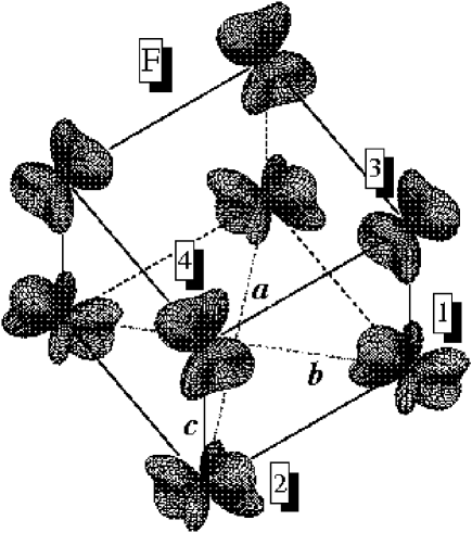
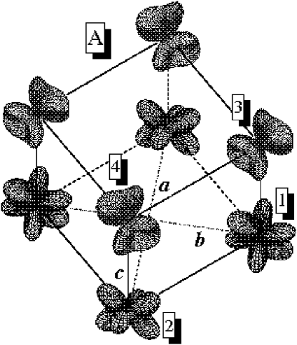
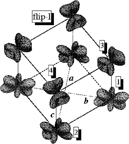
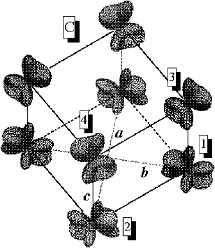
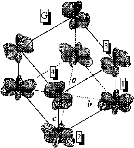
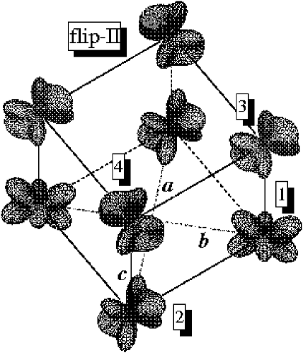
Figure 15: (Color online) Distribution of the charge density around V-sites in various magnetic phases of LaVO₃, as obtained in Hartree-Fock calculations . Different magnetic sublattices are shown by different colors.

Therefore, it is perhaps right to say that in LaVO₃, the experimental orbital ordering is partly driven by the magnetic ordering via the Kugel-Khomskii mechanism.KugelKhomskii This seems to agree with the experimental data, which show that in La-based compounds, the orbital ordering develops few degrees below the magnetic Néel temperature (T_N).Miyasaka This is again different from YVO₃, for which the orbital-ordering temperature is substantially higher than T_N.

The change of the orbital ordering is reflected in the behavior of interatomic magnetic interactions, which not only depend on the magnetic states, but can even change the signs (Table 6).

Table 6: Magnetic interactions ($J_{{\bf RR}^{\prime}}$), Hartree-Fock energies ($E_{\rm HF}$), and total energies ($E_{\rm tot}$) in LaVO₃. See Table 3 for other notations.

phase	$J_{12}$	$J_{13}$	$J_{24}$	$J_{34}$	$E_{\rm HF}$	$E_{\rm tot}$
F	$-$$5.1$	$6.6$	$6.6$	$-$$1.7$	$21.0$	$30.8$
A	$3.8$	$2.1$	$-$$4.5$	$-$$2.4$	$20.6$	$24.1$
C	$-$$4.8$	$6.0$	$6.0$	$-$$1.8$	$0$	$0$
G	$-$$6.3$	$-$$4.4$	$-$$4.4$	$-$$2.4$	$\phantom{1}7.6$	$11.1$
flip-I	$7.7$	$0.6$	$5.8$	$-$$1.7$	$\phantom{1}9.8$	$15.0$
flip-II	$-$$6.2$	$-$$4.0$	$5.8$	$-$$3.1$	$12.7$	$16.9$

In such a situation, the total energy may have several local minima, realized for those magnetic states where the signs of interatomic magnetic interactions are consistent with the type of the imposed spin ordering. We have found at least two such minima, corresponding to the C-type AFM ground state and the G-type AFM state, which has higher energy. Thus, we do not quite agree with the conclusions about the complete quenching of the orbital ordering in these distorted perovskite compounds.FangNagaosa This is not generally true and LaVO₃ is clearly an exception. However, the CF splitting will also prevent the formation of the orbital singlet states, which were employed in order to explain the appearance of the C-type AFM antiferromagnetism in the theory of orbital fluctuations.Khaliullin01 Actually, such a singlet state conflicts with the $C^{5}_{2h}$ symmetry of the monoclinic phase.

Since the interatomic magnetic interactions depend on the magnetic state, the simple Heisenberg model may be used only for the analysis of local perturbation around each magnetic state. Then, it is reasonable to expect a gap $\Delta_{\rm SW}$$\approx$$6.8$ meV between acoustic and optical branches of the spin-wave spectrum, similar to the one observed in the C-type AFM phase of YVO₃.Ulrich2003 However, the Heisenberg model is no longer valid for the analysis of the transition temperature (unlike in YTiO₃), which should take into account a possible change of the the orbital states in the course of thermodynamic average.

Similar to YVO₃ and YTiO₃, the correlation effects play a very important role also in LaVO₃ and additionally stabilize the C-type AFM ground state.

V.4 LaTiO₃

LaTiO₃ is a puzzling system. It has the smallest CF splitting (Fig. 8) among the distorted perovskite oxides, which formally leaves a room for the orbital fluctuations. On the other hand, the possible variation of the orbital order appears to be bounded by certain constraint conditions. For example, although the orbital ordering depends on the magnetic state, this dependence is not particularly large, as it is clearly seen from the HF calculations, where the basic shape of the orbital-ordering pattern remains the same for different magnetic states (Fig. 16).

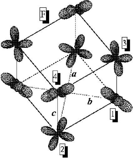
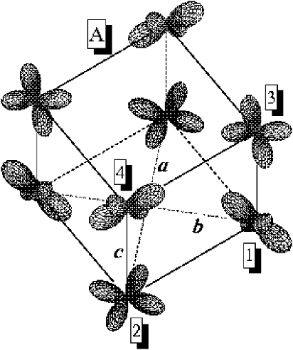
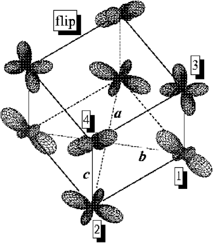
Figure 16: (Color online) Distribution of the charge density around Ti-sites in various magnetic phases of LaTiO₃, as obtained in Hartree-Fock calculations. Different magnetic sublattices are shown by different colors.

There are certainly some variations of the orbital ordering, which can be seen already on the plot. However, these variations do not seem to change the qualitative conclusion about the form of interatomic magnetic interactions and the magnetic ground state of LaTiO₃.

Unfortunately, this conclusion is not consistent with the experimental data. In this sense, there is a clear difference of LaTiO₃ from other perovskite compounds considered in this work, despite the fact that we have used absolutely the same procedure for construction and solution of the model Hamiltonian.

The magnetic ground state is expected to be of the A-type, as it is clearly seen from the total-energy calculations as well as from the behavior of interatomic magnetic interactions (Table 7), although experimentally, it is totally antiferromagnetic G-type.Keimer The magnetic interactions are sensitive to the magnetic ordering. However, other magnetic states appear to be unstable and the form of interatomic magnetic interactions in each magnetic state systematically leads to the A-type antiferromagnetism. This conclusion is totally consistent with results of our previous work,PRB04 which neglects the Madelung contribution to the CF splitting.

Table 7: Magnetic interactions ($J_{{\bf RR}^{\prime}}$), Hartree-Fock energies ($E_{\rm HF}$), total energies ($E_{\rm tot}$), and superexchange energies ($E_{\rm SE}$) in LaTiO₃. See Tables 3 and 5 for other notations.

phase	$J_{12}$	$J_{13}$	$J_{24}$	$J_{34}$	$E_{\rm HF}$	$E_{\rm tot}$	$E_{\rm SE}$
F	$4.5$	$-$$1.2$	$-$$1.2$	$4.5$	$\phantom{1}5.0$	$17.7$	$\phantom{1}1.6$
A	$3.6$	$-$$3.3$	$-$$3.3$	$3.6$	$0$	$0$	$0$
C	$1.0$	$-$$2.0$	$-$$2.0$	$3.4$	$19.6$	$26.3$	$14.2$
G	$2.0$	$-$$4.9$	$-$$4.9$	$2.0$	$11.5$	$11.0$	$\phantom{1}9.0$
flip	$1.3$	$-$$4.5$	$-$$0.4$	$4.6$	$\phantom{1}7.7$	$11.4$	$\phantom{1}5.7$

Then, what is missing in our calculations – or maybe even more generally – in our understanding of the magnetic properties of LaTiO₃? Below we discuss several plausible scenarios.
(i) One possibility is that the effect of the crystal distortion maybe still underestimated. Particularly, we tried to follow the idea of Refs. MochizukiImada, and Schmitz, , and additionally scaled the contribution of the Madelung term to the CF splitting by multiplying the right-hand side of Eq. (2) by a constant. This corresponds to the change of the dielectric constant, which was treated as an adjustable parameter in Refs. MochizukiImada, and Schmitz, . We have found that in order to obtain the experimental G-type antiferromagnetic ground state, the dielectric constant should be reduced by a factor four or five (Fig. 17).

Figure 17: (Color online) Total energies measured relative to the G-type antiferromagnetic state obtained in Hartree-Fock calculations with exaggerated crystal-field splitting of the Madelung type. The latter as been multiplied by the scaling factor shown in the absciss axis.

Then, the exchange interactions become nearly isotropic ($J_{12}$$=$$-$$3.3$ and $J_{13}$$=$$-$$3.5$ meV) and do not depend on the magnetic state. Hence, LaTiO₃ is expected to be a good Heisenberg antiferromagnet, in agreement with the experimental inelastic neutron-scattering data. The latter reveals nearly isotropic behavior of the spin-wave spectrum with $J_{12}=J_{13}=-$$15.5S^{2}\approx-$$3.9$ meV.Keimer Thus, we are totally agree with the authors of Refs. MochizukiImada, and Schmitz, that the Madelung term alone could explain many experimental features of LaTiO₃. The only problem is that, according to the electronic structure calculations, the effect is too small. One can of course try to blame LDA for this failure. However, why does this problem occur only for LaTiO₃ while for other compounds our method works reasonably well? We believe that if the story about the structural origin of the G-type antiferromagnetism in LaTiO₃ make a sense, it is more likely that the real magnitude of the crystal distortion in LaTiO₃ may be still undisclosed experimentally. This seems to be reasonable, because the structural data for the distorted perovskite oxides are still in the process of steady refinement.Blake ; Tsvetkov ; Cwik
(ii) Other scenarios are related with the correlation effects, which are not included in the HF calculations. There is no doubts that they must play an important role in LaTiO₃. However, it seems that there is no simple scheme which would allow to include these effects in the electronic structure calculations. The second-order perturbation theory and the theory of superexchange interactions, which we have tried, are definitely not enough. They do substantially change the total energies of the HF method. However, the conclusions strongly depend on the approximation which we use (Table 7). For example, from the second order perturbation theory, it seems to be clear that the correlation effects tend to stabilize the G-type AFM state: the correlations change the order of the magnetic states and somewhat lower the energy of the G-type AFM state relative to the A-state. The latter trend is also seen the superexchange approach. However, the superexchange method tends to lower also the energies of other magnetic states, apparently through the small change of the orbital ordering. This is in straight contrast with the more distorted YTiO₃, were two different methods provided rather consistent explanation for the role played by the correlation effects (Table 5).
(iii) The theory of orbital liquid is just an opposite case to the theory of CF splitting as these two effects are incompatible with each other. Although the formation of the orbital liquid in the cubic $t_{2g}$ lattice is a many-electron effect, the necessary prerequisite, which should exist already at the mean-field level, is an infinite degeneracy of the magnetic ground state.KhaliullinMaekawa Although our CF splitting for LaTiO₃ is small, that is sometimes regarded as the strong support for the orbital liquid theory, we do not observe such a degeneracy of the Hartree-Fock ground state: all HF calculations steadily converge to a single solution for the orbital-ordering pattern, which is shown in Fig. 16, irrespectively on the starting conditions and the size of the supercell. Therefore, although the correlation effects beyond the HF approximation are certainly important in the case of LaTiO₃, it does not necessary mean that the ultimate result of electron correlations must be formation of the orbital liquid state. We hope that even in LaTiO₃, the correlation effects can be systematically included using the regular perturbation theory expansion around the nondegenerate HF ground state, while the second order of this expansion is simply not enough. In such a situation, it is perhaps more practical to derive an approximate ground state from the diagonalization of a many-electron Hamiltonian matrix constructed in the basis of some limited number of specially selected Slater determinants, as it is done for example in the path-integral renormalization group method.Imai ; PIRG

Thus, one of the challenging problems in the theory of distorted perovskite oxides remains to be the explanation of the G-type AFM ground state in LaTiO₃. Definitely, we need a more rigorous theory for the correlation effects. But, will it be enough, or do we need a more radical refinement of our starting model, given by Eq. (1), in the case of LaTiO₃?

V.5 Spin-Orbit Interaction and Magnetic Ground State

The spin-orbit interaction in the distorted perovskite oxides will generally leads to the noncollinear spin arangement, which obeys certain symmetry rules.PhysicaB1997 The spin magnetic moments, aligned along one of the orthorhombic axes, will be subjected to certain rotational forces, coming both from the Dzyaloshinsky-Moriya interactions and from the single-ion anisotropy energies,DzyaloshinskyMoriya ; PRL96 which lead to the spin canting and the appearance of nonvanishing components of the spin-magnetization density along two other directions. The type of the magnetic ordering for all three projection of the spin-magnetization density is generally different. Thus, each magnetic structure can be generally abbreviated as $X$-$Y$-$Z$, where $X$, $Y$, and $Z$ is the type of the magnetic ordering (F, A, C, or G) formed by the projections of the spin magnetic moments onto the orthorhombic axes ${\bf a}$, ${\bf b}$, and ${\bf c}$, respectively. The orbital magnetic structure has the same symmetry, although it has a different origin of the canting, which comes mainly from the interplay of the spin-orbit interaction with the CF splitting at each transition site. The spin and orbital magnetic moments are not generally collinear to each other.PRB97

Results of HF calculations, which take into account the spin-orbit interaction, are summarized in Table 8.

Table 8: The type of the magnetic ground state, the vectors of the spin ($\bm{\mu}_{S}$) and orbital ($\bm{\mu}_{L}$) magnetic moments (in $\mu_{B}$), and the values of the band gap ($E_{g}$, in eV) obtained in Hartree-Fock calculations. For the magnetic ground state, three capital letters denote the type of the magnetic ordering for three projections of the magnetic moments onto the orthorhombic axes ${\bf a}$, ${\bf b}$, and ${\bf c}$, respectively. For the spin and orbital magnetic moments at the transition-metal sites, these three projections are specified by the vectors $\bm{\mu}_{S}$ and $\bm{\mu}_{L}$, respectively. The positions of the transition-metal sites are shown in Fig. 2.

compound	phase	site	ground state	$\bm{\mu}_{S}$	$\bm{\mu}_{L}$	$E_{g}$
YTiO3	o	1	G-A-F	($-$$0.00$,$-$$0.09$, $0.84$)	($-$$0.05$, $0.01$,$-$$0.03$)	$1.1$
LaTiO3	o	1	C-F-A	( $0.02$,$-$$0.17$, $0.76$)	( $0.10$, $0.03$,$-$$0.08$)	$0.6$
YVO3	o	1	F-C-G	($-$$0.02$, $0.00$, $1.65$)	( $0.00$,$-$$0.00$,$-$$0.17$)	$1.2$
YVO3	m	1	C-A-C	($-$$0.74$, $0.08$, $1.48$)	( $0.07$,$-$$0.04$,$-$$0.16$)	$1.0$
		3		($-$$0.78$,$-$$0.03$, $1.48$)	( $0.05$, $0.04$,$-$$0.07$)
LaVO3	m	1	A-C-A	($-$$0.05$, $1.64$,$-$$0.05$)	( $0.09$,$-$$0.18$, $0.11$)	$0.9$
		3		( $0.06$, $1.63$, $0.05$)	($-$$0.05$,$-$$0.09$,$-$$0.06$)

The magnetic ground state of YTiO₃ is G-A-F, in agreement with the neutron scattering data.Ulrich2002 The ferromagnetic moment is aligned along the ${\bf c}$-axis, and the canting angle is relatively small. The absolute values of the spin and orbital magnetic moments are different from those reported in our previous work.PRB04 The difference is related with the additional transformation to the LMTO basis, which allows to calculate the local magnetic moments directly at the transition-metal sites, whereas in Ref. PRB04, they have been calculated in the Wannier basis, which had a substantial weight at the oxygen sites. This comparison clearly shows that the covalent effects play a very important role and allow to explain a substantial reduction of the local magnetic moments at the transition-metal sites. As it was already discussed in Sec. V.2, the correlation effects in YTiO₃ favor the AFM coupling and systematically lower the energies of all AFM states relative to the ferromagnetic one (see Table 5). After including the spin-orbit interaction, this will lead to the additional spin canting away from the collinear ferromagnetic arrangement. For example, in the framework of superexchange approach we have obtained the following values of the spin and orbital magnetic moments (in $\mu_{B}$, referred to the site 1): $\bm{\mu}_{S}$$=$$(-0.02,-0.29,\phantom{-}0.77)$ and $\bm{\mu}_{L}$$=$$(-0.05,\phantom{-}0.02,-0.03)$. It readily explains the experimental values reported for the F and G components of the magnetic moments, correspondingly along the ${\bf c}$ and ${\bf a}$-directions,Ulrich2002 while the A-type AFM component along the ${\bf b}$-direction is somewhat larger in our calculations. The reason is not completely clear. The orbital magnetic moments in YTiO₃ are strongly quenched by the crystal field.

The orthorhombic YVO₃ has nearly-collinear magnetic structure, where the G-type AFM moment is aligned along the ${\bf c}$-axis. The total magnetic moment $(\bm{\mu}_{S}$$+$$\bm{\mu}_{L})\|{\bf c}$$=$$1.48\mu_{B}$ parallel to the ${\bf c}$-axis is in excellent agreement with the experimental value of $1.45\mu_{B}$ reported by Blake et al. and corresponding to T$=$$65$ K.Blake Ulrich et al. reported somewhat larger value of $1.72\mu_{B}$, also oriented along ${\bf c}$. The weak ferromagnetic component along the ${\bf a}$-direction has been also observed experimentally.Ren Details of magnetic ordering in the monoclinic phase of YVO₃ are somewhat controversial. Blake et al. reported the C-type AFM ordering for both ${\bf b}$- and ${\bf c}$-components of the magnetic moments in the orthorhombic $Pbnm$ notations, which correspond to the ${\bf a}$- and ${\bf c}$-directions in the monoclinic $P2_{1}/a$ notations.Blake This is totally consistent with our finding. The quantitative difference can be naturally explained by the finite temperature effects in the intermediate phase.FangNagaosa Furthermore, we predict the A-type antiferrimagnetic ordering for the remaining ${\bf b}$-component (in the $P2_{1}/a$ notations), which implies nearly antiferromagnetic alignment of the ${\bf b}$-projections of the magnetic moments in the adjacent ${\bf ab}$-planes. However, since the sites $1$ and $3$ are not fully equivalent in the monoclinic structure, the ${\bf b}$-projections do not compensate each other, and the system exposes the net magnetic moment, which can couple to the magnetic field.Ren The antiferrimagnetic ordering along the ${\bf b}$-axis is also consistent with the temperature-induced magnetization reversal behavior of YVO₃ observed by Ren,Ren and could be a natural explanation for this effect. More generally, it is right to say that the magnetic coupling along the ${\bf c}$-direction of the monoclinic phase is always either ferrimagnetic or antiferrimagnetic, because the sites $1$ and $3$ are not equivalent.

The C-A-C magnetic ground state appears to be different from the magnetic structure reported by Ulrich et al., who have observed the C-type AFM ordering for the ${\bf a}$- and ${\bf b}$-components, and the G-type AFM ordering for the remaining ${\bf c}$-component (apparently, in the $Pbnm$ notations).Ulrich2003 One possible explanation for this difference could be the coexistence of several magnetic states in a narrow energy range. Such a behavior has been indeed observed in our HF calculations: in addition to the C-A-C state we could obtain another self-consistent solution corresponding to the A-C-F phase with a slightly higher energy (about $0.04$ meV per one formula unit, which is of the order of the magnetocrystalline anisotropy energy). The new phase has the following magnetic moments (in $\mu_{B}$, where the first and second lines corresponds to the sites $1$ and $3$, respectively):

$$\begin{array}[]{cc}\bm{\mu}_{S}^{1}=(-0.07,\phantom{-}1.65,\phantom{-}0.05),&\bm{\mu}_{L}^{1}=(\phantom{-}0.05,-0.15,-0.02),\\ \bm{\mu}_{S}^{3}=(\phantom{-}0.07,\phantom{-}1.67,\phantom{-}0.03),&\bm{\mu}_{L}^{3}=(-0.09,-0.07,-0.02).\\ \end{array}$$

Although the exact form of the magnetic state A-C-F is still different from the observation by Ulrich et al.,Ulrich2003 we can speculate that they probably used a different experimental setup which yielded the realization of another magnetic phase, which was different from the finding by Blake et al. (Ref. Blake, ) and Ren et al. (Ref. Ren, ). At least, the C-type AFM component parallel to the ${\bf ab}$-plane is qualitatively consistent with the form of the A-C-F phase obtain in our HF conclusions, and to certain extent the results of HF calculations can be further modified by the correlation effects.

In the case of LaVO₃ we could find three stable solutions: A-C-A, C-A-C, and C-F-G. The first two are similar to the A-C-F and C-A-C states, emerging in monoclinic YVO₃. The only difference is that the A-C-A state has lower energy and, therefore, is realized as the ground state in the case of LaVO₃. Like in YVO₃, the A-type state corresponds to the antiferrimagnetic ordering. Therefore, LaVO₃ is expected to have the net magnetic moment in the ${\bf ac}$-plane. The third (C-F-G) solution has nearly collinear spin structure:

$$\begin{array}[]{cc}\bm{\mu}_{S}^{1}=(-0.01,-0.06,\phantom{-}1.60),&\bm{\mu}_{L}^{1}=(\phantom{-}0.01,\phantom{-}0.13,-0.34),\\ \bm{\mu}_{S}^{3}=(-0.03,-0.02,-1.61),&\bm{\mu}_{L}^{3}=(\phantom{-}0.01,\phantom{-}0.04,\phantom{-}0.14).\\ \end{array}$$

It corresponds to the stable G-type AFM phase emerging without the spin-orbit interaction (see Table 3). Nevertheless, the A-C-A state appears to be well separated from the C-A-C and C-F-G states, correspondingly by $0.19$ and $6.50$ meV per one formula unit.

The quenching of the orbital magnetic moments in two different sublattices of monoclinic YVO₃ and LaVO₃ nicely correlates with the values of the CF splitting (Fig. 8), where larger CF splitting at the site 3 results in smaller orbital magnetization.

It is probably meaningless to discuss the relativistic effects in LaTiO₃, where we could not reproduce the correct magnetic ground state. We could agree with the criticism risen by Haverkort et al. (Ref. Haverkort, ) that our CF splitting alone does not explain details of their spin-resolved photoemission spectra (actually, our value of the parameter $\langle{\bf L}\cdot{\bf S}\rangle$, obtained in the HF calculations after the transformation to the LMTO basis and radial integration over the Ti-sphere is about $-$$0.13$, which exceeds the experimental value by factor two). However, it does not make a sense to present as an alternative the results of calculations yielding the same A-type AFM ground state,Streltsov which totally agrees with our finding and (unfortunately) disagrees with the experiment, even though these calculations yield somewhat larger value of the CF splitting for LaTiO₃. As it has been already discussed in Sec. III.1, different values of the CF splitting obtained by different authors are most probably related with the nonunique choice of the Wannier functions for the $t_{2g}$ bands of the distorted perovskite oxides. One can formally adjust the theoretical CF splitting in order to meet certain demands of some particular class of the experimental data. However, will it solve a more fundamental problem of the magnetic ground state of LaTiO₃?

In addition, we show in Table 8 the values of the band gap obtained in the HF calculations for the magnetic ground state. For YTiO₃, YVO₃, and LaVO₃ there is a good agreement with the experimental optical data.Tsvetkov ; optics_exp However, for LaTiO₃ the experimental gap is much smaller ($\sim$$0.1$ eV).optics_exp This may indicate again at the particular importance of correlation effects in LaTiO₃.

VI Summary and Concluding Remarks

The main purpose of this work was to make a bridge between first-principles electronic structure calculations and model approaches for the strongly-correlated systems, and illustrate how it works for the series of distorted $t_{2g}$ perovskite oxides. The whole plan included three major steps: first-principles electronic structure calculations $\rightarrow$ construction of the model Hamiltonian for the isolated $t_{2g}$ bands near the Fermi level $\rightarrow$ solution of this model Hamiltonian using several different approaches. The choice of the distorted $t_{2g}$ perovskite oxides was motivated by the fact that they represent a good example of systems where it is practically impossible to construct a relevant model without the impact from the first-principles calculations: simply, the lattice distortion is too complex and there are too many model parameters, which cannot be fixed in unbiased way. In this sense, we strongly believe that any theoretical model for such complex oxide materials should be based on the results of first-principles electronic structure calculations. Otherwise it could be just an abstract mathematical construction deprived of clear physical grounds.

The present work clearly demonstrates that nowadays the idea of constructing the parameter-free model Hamiltonians for the strongly-correlated systems is quite feasible: all model parameters in our work, including the intraatomic Coulomb interactions, have been derived from the first-principles calculations using the method proposed in Ref. condmat05, . Apart from the approximations inherent to the method, the procedure of constructing the model Hamiltonian was totally parameter-free, and our analysis did not rely on the use of any adjustable parameters. Therefore, it is remarkable that using such a parameter-free approach we could propose a consistent explanation for a number of puzzling properties of the distorted $t_{2g}$ perovskite oxides. These first results are really encouraging and we would like to hope that the method proposed in Ref. condmat05, can be successfully applied in the future for the analysis of electronic and magnetic properties of other narrow-band compounds.

At the mean-field Hartree-Fock level, the results of all-electron full-potential LDA$+$$U$ calculations (Refs. SawadaTerakura, ; FangNagaosa, ) can be successfully reproduced in our model approach for the isolated $t_{2g}$ bands. We could easily rationalize the main results of these relatively heavy calculations and elucidate the main microscopic interactions responsible for the formation of different magnetic structures in the case of YTiO₃, YVO₃, and LaVO₃. We argue that the nonsphericity of the Madelung potential should be an indispensable ingredient of electronic structure calculations, and the results of commonly used atomic-spheres-approximation should be corrected in order to include these effects.

The crystal distortion plays an important role in the physics of $t_{2g}$ perovskite oxides. At least for YTiO₃, YVO₃, and LaVO₃, the knowledge of the experimental lattice parameters and the atomic positions greatly helps in explaining the magnetic properties of these compounds. Of course, some questions still remain. Particularly, what is the origin of this distortion? Why is it so different for different compounds, that is finally manifested in the formation of completely different magnetic structures? Very similar arguments have been used for LaMnO₃, which is a characteristic example of the Jahn-Teller distorted $e_{g}$ perovskite oxides. Particularly, it was argued that the experimental distortion not only stabilize the A-type AFM ground state of LaMnO₃,PRL96 ; LaMnO3_band ; Maezono ; GorkovKresin but is also responsible for the opening of the band gap.LaMnO3_band ; GorkovKresin However, the direction of the Jahn-Teller distortion in LaMnO₃ can be naturally understood in terms of anharmonicity of the electron-lattice interaction.KugelKhomskii ; Kanamori3 ; Millis In this sense, LaMnO₃ is an easy example. Then, is it possible to rationalize the behavior of $t_{2g}$ perovskite oxides in a similar way and come up with some suitable electron-lattice model, which would explain not only the direction of the lattice distortion in each particular compound, but also the difference between these compounds?

Finally, we emphasize the importance of correlation effects in the $t_{2g}$ band of distorted perovskite oxides. Although the mean-field Hartree-Fock approach provides a satisfactory description for the magnetic properties of YTiO₃, YVO₃, and LaVO₃, the inclusion of the correlation effects systematically improves the agreement with the experimental data for all three compounds. Definitely, LaTiO₃ is an exceptional example for which we could not obtain the correct G-type AFM ground state neither at the level of Hartree-Fock approach nor after including some correlation effects, though in a very approximate form. However, we expect that the situation may still change by systematically employing more rigorous theories for the correlation effects. The approximations considered in the present work were simply not enough in the case of LaTiO₃.

- (1) M. Imada, A. Fujimori, and Y. Tokura, Rev. Mod. Phys. 70, 1039 (1998); Y. Tokura and N. Nagaosa, Science 288, 462 (2000).
- (2) V. I. Anisimov, J. Zaanen, and O. K. Andersen, Phys. Rev. B 44, 943 (1991).
- (3) I. V. Solovyev, P. H. Dederichs, and V. I. Anisimov, Phys. Rev. B 50, 16861 (1994).
- (4) V. I. Anisimov, A. I. Poteryaev, M. A. Korotin, A. O. Anokhin, and G. Kotliar, J. Phys. Condens. Matt. 9, 7359 (1997); S. Y. Savrasov, G. Kotliar, and E. Abrahams, Nature 410, 793 (2001); K. Held, G. Keller, V. Eyert, D. Vollhardt, and V. I. Anisimov, Phys. Rev. Lett. 86, 5345 (2001); A. I. Lichtenstein and M. I. Katsnelson, Phys. Rev. B 57, 6884 (1998).
- (5) Y. Imai, I. Solovyev, and M. Imada, Phys. Rev. Lett. 95, 176405 (2005).
- (6) D. A. Maclean, H.-N. Ng, and J. E. Greedan, J. Solid State Chem. 30, 35 (1979).
- (7) M. Itoh, M. Tsuchiya, H. Tanaka, and K. Motoya, J. Phys. Soc. Jpn. 68, 2783 (1999).
- (8) J. Akimitsu, H. Ichikawa, N. Eguchi, T. Miyano, M. Nishi, and K. Kakurai, J. Phys. Soc. Jpn. 70, 3475 (2001).
- (9) C. Ulrich, G. Khaliullin, M. Reehuis, A. Ivanov, H. He, Y. Taguchi, Y. Tokura, and B. Keimer, Phys. Rev. Lett. 89, 167202 (2002).
- (10) F. Iga, M. Tsubota, M. Sawada, H. B. Huang, S. Kura, M. Takemura, K. Yaji, M. Nagira, A. Kimura, T. Jo, T. Takabatake, H. Namatame, and M. Taniguchi, Phys. Rev. Lett. 93, 257207 (2004).
- (11) B. Keimer, D. Casa, A. Ivanov, J. W. Lynn, M. v. Zimmermann, J. P. Hill, D. Gibbs, Y. Taguchi, and Y. Tokura, Phys. Rev. Lett. 85, 3946 (2000).
- (12) M. Cwik, T. Lorenz, J. Baier, R. Müller, G. André, F. Bourée, F. Lichtenberg, A. Freimuth, R. Schmitz, E. Müller-Hartmann, and M. Braden, Phys. Rev. B 68, 060401(R) (2003).
- (13) Y. Ren, T. T. M. Palstra, D. I. Khomskii, E. Pellegrin, A. A. Nugroho, A. A. Menovsky, and G. A. Sawatzky, Nature 396, 441 (1998).
- (14) G. R. Blake, T. T. Palstra, Y. Ren, A. A. Nugroho, and A. A. Menovsky, Phys. Rev. B 65, 174112 (2002).
- (15) A. A. Tsvetkov, F. P. Mena, P. H. M. van Loosdrecht, D. van der Marel, Y. Ren, A. A. Nugroho, A. A. Menovsky, I. S. Elfimov, and G. A. Sawatzky, Phys. Rev. B 69, 075110 (2004).
- (16) C. Ulrich, G. Khaliullin, J. Sirker, M. Reehuis, M. Ohl, S. Miyasaka, Y. Tokura, and B. Keimer, Phys. Rev. Lett. 91, 257202 (2003).
- (17) V. G. Zubkov, G. V. Bazuev, V. A. Perelyaev, and G. P. Shveikin, Sov. Phys. Solid State 15, 1079 (1973).
- (18) P. Bordet, C. Chaillout, M. Marezio, Q. Huang, A. Santoro, S-W. Cheong, H. Takagi, C. S. Oglesby, and B. Batlogg, J. Solid State Chem. 106, 235 (1993).
- (19) T. Mizokawa and A. Fujimori, Phys. Rev. B 54, 5368 (1996).
- (20) G. Khaliullin and S. Maekawa, Phys. Rev. Lett. 85, 3950 (2000).
- (21) G. Khaliullin, P. Horsch, and A. M. Oleś, Phys. Rev. Lett. 86, 3879 (2001).
- (22) G. Khaliullin and S. Okamoto, Phys. Rev. Lett. 89, 167201 (2002).
- (23) M. Mochizuki and M. Imada, Phys. Rev. Lett. 91, 167203 (2003).
- (24) R. Schmitz, O. Entin-Wohlman, A. Aharony, A. B. Harris, and E. Müller-Hartmann, Phys. Rev. B 71, 144412 (2005).
- (25) H. Fujitani and S. Asano, Phys. Rev. B 51, 2098 (1995).
- (26) H. Sawada, N. Hamada, K. Terakura, and T. Asada, Phys. Rev. B 53, 12742 (1996).
- (27) H. Sawada and K. Terakura, Phys. Rev. B 58, 6831 (1998).
- (28) I. V. Solovyev, Phys. Rev. B 69, 134403 (2004).
- (29) Z. Fang and N. Nagaosa, Phys. Rev. Lett. 93, 176404 (2004).
- (30) E. Pavarini, S. Biermann, A. Poteryaev, A. I. Lichtenstein, A. Georges, and O. K. Andersen, Phys. Rev. Lett. 92, 176403 (2004).
- (31) E. Pavarini, A. Yamasaki, J. Nuss, and O. K. Andersen, New Journal of Physics 7, 188 (2005).
- (32) S. V. Streltsov, A. S. Mylnikova, A. O. Shorikov, Z. V. Pchelkina, D. I. Khomskii, and V. I. Anisimov, Phys. Rev. B 71, 245114 (2005).
- (33) S. Okatov, A. Poteryaev, and A. Lichtenstein, cond-mat/0412063.
- (34) I. V. Solovyev, cond-mat/0506632.
- (35) There are certain indications that the actual symmetry of the intermediate phase of YVO3 can be even lower than .Tsvetkov
- (36) For example, from the viewpoint of superexchange interactions, it is more natural to define the “orthogonal” orbitals as the ones which are decoupled via the matrix of transfer integrals between neighboring transition-metal sites: , which is not always the same as the regular orthogonality condition.PRB04
- (37) O. K. Andersen, Phys. Rev. B 12, 3060 (1975); O. Gunnarsson, O. Jepsen, and O. K. Andersen, ibid. 27, 7144 (1983); H. L. Skriver, The LMTO Method, (Springer-Verlag, Berlin, 1984); O. K. Andersen, Z. Pawlowska, and O. Jepsen, Phys. Rev. B 34, 5253 (1986).
- (38) The Wannir functions have been calculated using the method proposed in Ref. condmat05, . In these calculations, the Wannier functions for the bands have been orthogonalized to the O(), Ti(), and Y() bands, in the case of YTiO3; O(), Ti(), and La() bands, in the case of LaTiO3; O(), V(), and Y() bands, in the case of YVO3; and O(), V(), and La() bands, in the case of LaVO3. We have confirmed that such a accuracy is sufficient for calculations of the crystal-field splitting caused by the nonsphericity of the Madelung potential (2).
- (39) N. Marzari and D. Vanderbilt, Phys. Rev. B 56, 12847 (1997).
- (40) J. Kanamori, Prog. Theor. Phys. 17, 177 (1957).
- (41) M. W. Haverkort, Z. Hu, A. Tanaka, G. Ghiringhelli, H. Roth, M. Cwik, T. Lorenz, C. Schüssler-Langeheine, S. V. Streltsov, A. S. Mylnikova, V. I. Anisimov, C. de Nadai, N. B. Brookes, H. H. Hsieh, H.-J. Lin, C. T. Chen, T. Mizokawa, Y. Taguchi, Y. Tokura, D. I. Khomskii, and L. H. Tjeng, Phys. Rev. Lett. 94, 056401 (2005).
- (42) C. J. Bradley and A. P. Cracknell, The Mathematical Theory of Symmetry in Solids (Clarendon Press, Oxford, 1972).
- (43) Note that in order to improve ASA for the loosely packed atomic structures, several empty spheres have been added in the process of LMTO calculations. A typical example for YTiO3 is given in Ref. condmat05, . These spheres are negatively charged () and some of them are located in the nearest neighborhood to the transition-metal sites. The contribution of these spheres to the Madelung potential makes some difference from the conventional form of the CF splitting expected from the the point-charge model.
- (44) O. Gunnarsson, O. K. Andersen, O. Jepsen, and J. Zaanen, Phys. Rev. B 39, 1708 (1989); O. Gunnarsson, A. V. Postnikov, and O. K. Andersen, ibid. 40, 10407 (1989); V. I. Anisimov and O. Gunnarsson, ibid. 43, 7570 (1991); I. V. Solovyev and P. H. Dederichs, ibid. 49, 6736 (1994).
- (45) J. Kanamori, Prog. Theor. Phys. 30, 275 (1963). Note that the definition of the Kanamori parameters and is different from the parameters and , which are typically used in LDA calculations.PRB94 Nevertheless, there is a simple relation connecting these two sets of parameters: and .
- (46) A. I. Liechtenstein, M. I. Katsnelson, V. P. Antropov, and V. A. Gubanov, J. Magn. Magn. Matter. 67, 65 (1987); I. V. Solovyev, in Recent Research Developments in Magnetism and Magnetic Materials (Transworld Research Network, India, 2003), Vol. 1, pp. 253-294.
- (47) J. Friedel and C. M. Sayers, J. Physique 38, 697 (1977); F. Kajzar and J. Friedel, ibid. 39, 397 (1978); G. Treglia, F. Ducastelle, and D. Spanjaard, ibid. 41, 281 (1980).
- (48) A. Georges, G. Kotliar, W. Krauth, and M. J. Rozenberg, Rev. Mod. Phys. 68, 13 (1996).
- (49) R. Shiina, T. Nishitani, and H. Shiba, J. Phys. Soc. Jpn. 66, 3159 (1997); L. F. Feiner and A. M. Oleś, Phys. Rev. B 59, 3295 (1999).
- (50) P. W. Anderson, Phys. Rev. 115, 2 (1959).
- (51) K. I. Kugel and D. I. Khomskii, Sov. Phys. Usp. 25, 231 (1982).
- (52) Note that . Therefore, according to Eq. (12), two separate excitations into the singlet (S) and triplet (T) states are more favorable energetically rather than the excitation into the Hartree-Fock state with an averaged energy.
- (53) M. Noguchi, A. Nakazawa, S. Oka, T. Arima, Y. Wakabayashi, H. Nakao, and Y. Murakami, Phys. Rev. B 62, R9271 (2000).
- (54) Note, however, that the LDA calculations reported in Refs. SawadaTerakura, and FangNagaosa, for YVO3 overestimate the total energy difference between different magnetic states, apparently due to the double-counting of the nonsphericity effects. By default, in the full-potential implementation of the LDA method, the nonsphericity of the on-site Coulomb and exchange-correlation potential is taken into account twice: in the LDA-part and in the correction for the on-site Coulomb interactions. Therefore, the LDA-part should be additionally averaged inside some atomic sphere and we belive that it is more physical to treat this part in ASA.condmat05 This problem mainly concerns with the compounds, which are subjected to the Hund’s rule effects coming from the nonspherical Coulomb interactions between two electrons. A more general problem is related with the technical implementations of the LDA method (e.g. the choice of the parameter and the basis orbitals for the correction), which probably explain a small difference existing between our results and Ref. SawadaTerakura, for YTiO3.
- (55) and , where is the total energy either in the pure HF approximation or after including the correlation effects in the second order of perturbation theory.
- (56) E. L. Nagaev, Magnetics with Complex Magnetic Interactions (Science, Moscow, 1988).
- (57) Note that our scheme of calculation of the exchange parameters is based on the infinitesimal rotations of the spin magnetic moments, which implies that the spins are classical. Therefore, the total energy of the Heisenberg model has the form (8), where are related with the regular Heisenberg parameters as . Therefore, to be consistent we our definition of the exchange parameters, we use the classical expression also for the transition temperature and replace by . In order to use the quantum-mechanical definition for the transition temperature, one should do a proper mapping of the total-energy change onto the Heisenberg model, which is much more complex, because in quantum case, the total energy remains proportional to only for the ferromagnetically coupled spins. The antiferromagnetic arangement yields an additional prefactor , which is specific to the geometry of the system and bounded by the following conditions: . The latter are far from restrictive when the spin is small. Therefore, the quantum effects, which are especially important for the spin , will modify not only the expression for the transition temperature, but also the definition of the parameters of the Heisenberg model themselves.
- (58) N. D. Mermin and H. Wagner, Phys. Rev. Lett. 17, 1133 (1966); 17, 1307(E) (1966).
- (59) S. Miyasaka, Y. Okimoto, M. Iwama, and Y. Tokura, Phys. Rev. B 68, 100406 (2003).
- (60) M. Imada and T. Kashima, J. Phys. Soc. Jpn. 69, 2723 (2000); T. Kashima and M. Imada, ibid. 70, 2287 (2001); T. Mizusaki and M. Imada, Phys. Rev. B 69, 125110 (2004).
- (61) D. Treves, Phys. Rev. 125, 1843 (1962); A. S. Moskvin and E. V. Sinitsyn, Sov. Phys. Solid State 14, 2198 (1973); T. Yamaguchi, J. Chem. Phys. Solids 35, 479 (1974); I. V. Solovyev, N. Hamada, and K. Terakura, Physica B 237-238, 44 (1997).
- (62) I. Dzyaloshinsky, J. Chem. Phys. Solids 4, 241 (1958); T. Moriya, Phys. Rev. 120, 91 (1960).
- (63) I. Solovyev, N. Hamada, and K. Terakura, Phys. Rev. Lett. 76, 4825 (1996).
- (64) I. V. Solovyev, Phys. Rev. B 55, 8060 (1997).
- (65) T. Arima, Y. Tokura, and J. B. Torrance, Phys. Rev. B 48, 17006 (1993); Y. Okimoto, T. Katsufuji, Y. Okada, T. Arima, and Y. Tokura, Phys. Rev. B 51, 9581 (1995); S. Miyasaka, Y. Okimoto, and Y. Tokura, J. Phys. Soc. Jpn. 71, 2086 (2002).
- (66) N. Hamada, H. Sawada, and K. Terakura (1995): in Spectroscopy of Mott Insulators and Correlated Metals, edited by A. Fujimori and Y. Tokura (Springer, Berlin, 1995); W. E. Pickett and D. J. Singh, Phys. Rev. B 53, 1146 (1996); I. V. Solovyev and K. Terakura, in Electronic Structure and Magnetism of Complex Materials, ed. by D. J. Singh and D. A. Papaconstantopoulos (Springer, Berlin, 2003).
- (67) R. Maezono, S. Ishihara, and N. Nagaosa, Phys. Rev. B 58, 11583 (1998).
- (68) L. P. Gor’kov and V. Z. Kresin (1998), JETP Lett. 67, 985 (1998).
- (69) J. Kanamori, J. Appl. Phys. Suppl. 31, 14S (1960).
- (70) A. J. Millis, Phys. Rev. B 53, 8434 (1996).