Frequency-Dependent Current Noise through Quantum-Dot Spin Valves

Abstract

We study frequency-dependent current noise through a single-level quantum dot connected to ferromagnetic leads with non-collinear magnetization. We propose to use the frequency-dependent Fano factor as a tool to detect single-spin dynamics in the quantum dot. Spin precession due to an external magnetic and/or a many-body exchange field affects the Fano factor of the system in two ways. First, the tendency towards spin-selective bunching of the transmitted electrons is suppressed, which gives rise to a reduction of the low-frequency noise. Second, the noise spectrum displays a resonance at the Larmor frequency, whose lineshape depends on the relative angle of the leads’ magnetizations.

I Introduction

The measurement of current noise reveals additional information about mesoscopic conductors that is not contained in the average current.review ; review2 Current noise through quantum dots exposes the strongly-correlated character of charge transport due to Coulomb interaction, giving rise to phenomena such as positive cross correlations,cottet and sub- or super-Poissonian Fano factors.superpoissonian1 ; superpoissonian2 This is one motivation for the extensive theoreticalkorotkov ; hershfield ; hanke ; thielmann ; Lue and experimentalexperiment ; haug1 ; haug2 study of zero- and finite-frequency noise of the current through quantum dots. Furthermore, the finite-frequency noise provides a direct access to the internal dynamics of the system such as coherent oscillations in double-dot structures,gurvitz2 ; bingdong ; Sun ; Kieslich quantum-shuttle resonances,flindt transport through a dot with a precessing magnetic moment,precessingspin or back action of a detector to the system.backaction1 ; backaction2 ; backaction3

In this paper, we investigate the transport through a single-level quantum dot connected to ferromagnetic leads with non-collinear magnetizations in the limit of weak dot-lead coupling, see Fig. 1. Recent experimental approaches to contact a quantum dot to ferromagnetic leads involve metallic islands, ono ; wees granular systems, grain_experiment ; granular carbon nanotubes cnt ; schoenenberger as well as single molecules ralph2 or self-assembled quantum dots.QD-exp ; ralph Quantum-dot spin-valve structures are interesting, since the presence of both a finite spin polarization in the leads and an applied bias voltage induces, for a non-parallel alignment of the lead magnetization directions, an non-equilibrium spin on the quantum dot. The magnitude and direction of the quantum-dot spin is determined by the interplay of two processes: non-equilibrium spin accumulation due to spin injection from the leads, and spin precession due to an exchange field generated by the tunnel coupling to spin-polarized leadsbraun1 or due to an externally applied magnetic field.braun2 The resulting average quantum-dot spin affects the $dc-$conductance of the device.

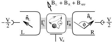
Figure 1: A quantum dot contacted by ferromagnetic leads with non-collinear magnetizations. Electrons polarized along the source (left) lead enter the dot. During their stay on the dot, the spins precess in the many-body exchange field $\bm{B}_{\rm L}+\bm{B}_{\rm R}$, which arises from the tunnel coupling to the left and right lead, and an applied magnetic field $\bm{B}_{\rm app}$. Due to magnetoresistance effects this precession modulates the tunnel-out probability to the drain (right) lead, giving rise to a signal in the power spectrum of the current noise.

While the time-averaged current is sensitive to the time-averaged dot spin, the time-resolved dynamics of the dot spin is provided by the power spectrum of the current noise. It will show a signature at the frequency that is associated with the precession of the quantum-dot spin due to the sum of exchange and external magnetic field. This can be understood by looking at the tunneling-out current to the drain (right) lead as a function of the time after the quantum-dot electron had tunneled in from the source (left) lead. The spin of the incoming electron, defined by the source-lead magnetization direction, precesses about the sum of exchange and external magnetic field as long as it stays in the dot. Since the tunneling-out rate depends on the relative orientation of the quantum-dot spin to the drain-lead magnetization direction, the spin precession leads to a periodic oscillation of the tunneling-out probability. The period of the oscillation is defined by the inverse precession frequency, and the phase is given by the relative orientation of the source- and drain-lead magnetization direction. As a consequence, the signature in the power spectrum of the current noise at the Larmor frequency gradually changes from a peak to a dip as a function of angle between source- and drain-lead magnetization.

Also the zero-frequency part of the current-noise power spectrum is affected by the internal dynamics of the quantum-dot spin. By coupling a quantum dot to spin-polarized electrodes, the dwell time of the electrons in the dot becomes spin dependent. It is knownBulka1999 ; cottet that this spin dependence of the dwell times yields a bunching of the transferred electrons, which leads to an increase of the shot noise. A precession of the quantum-dot spin due to exchange and external magnetic field weakens the tendency towards bunching, leading to a reduction of the low-frequency noise.

The aim of this paper is to perform a systematic study of the frequency-dependent current noise of a quantum-dot spin valve in the limit of weak dot-lead coupling in order to illustrate the effects formulated above. In Sec. II we define the model of a quantum-dot spin valve, as shown in Fig. 1. In Sec. III, we extend a previously-developed diagrammatic real-time techniquediagrams to evaluate frequency-dependent current noise, as it has been similarly done for metallic (non-magnetic) single-electron transistors.johansson ; backaction1 The results for the quantum-dot spin valve are discussed in Sec. IV, followed by the Conclusions in Sec. V.

II Model System

The Hamiltonian for the quantum-dot spin valve, i.e., a quantum dot coupled to ferromagnetic leads, is given by the sum

$$H=H_{\rm L}+H_{\rm R}+H_{\rm D}+H_{\rm T}\,.$$ (1)

The single-level quantum dot is modeled by an Anderson impurity,

$$H_{\rm D}=\sum_{\sigma=\uparrow\downarrow}\varepsilon_{\sigma}c^{{\dagger}}_{\sigma}c_{\sigma}+U\,n_{\uparrow}n_{\downarrow}\,,$$ (2)

where $c^{{\dagger}}_{\sigma}$ and $c_{\sigma}$ are the fermion creation and annihilation operators of the dot electrons, and $n_{\sigma}=c^{{\dagger}}_{\sigma}c_{\sigma}$. The single-particle level at the energy $\varepsilon$, measured relative to the equilibrium Fermi energy of the leads, may be split due to an external magnetic field, $\varepsilon_{\uparrow}=\varepsilon+\Delta/2$ and $\varepsilon_{\downarrow}=\varepsilon-\Delta/2$ with Zeeman energy $\Delta=g\mu_{\rm B}B_{\rm ext}$. Double occupancy of the dot costs the charging energy $U\gg k_{\rm B}T$.

The ferromagnetic leads $(r=\rm L/R)$ are treated as reservoirs of non-interacting fermions,

$$H_{r}=\sum_{k,\alpha=\pm}\varepsilon^{\,}_{k\alpha}a^{{\dagger}}_{rk\alpha}a^{\,}_{rk\alpha}\,.$$ (3)

By choosing the quantization axis of each lead parallel to their direction of magnetization ${\bf\hat{n}}_{r}$, the property of ferromagnetism can be included by assuming different density of states $\xi_{\alpha}$ for majority $(\alpha=+)$ and minority $(\alpha=-)$ electrons. An applied bias voltage is incorporated by a symmetric shift of the chemical potential by $\mu_{\rm L/R}=\pm eV/2$ in the left and right lead, which enter the Fermi functions $f_{r}(E)=f(E-\mu_{r})$.

The magnetization directions of the left and right lead and the external magnetic field are, in general, non-collinear, i.e., in the Hamiltonians for the three subsystems we have chosen different spin quantization axes. To describe spin-conserving tunneling, one must include $SU(2)$ rotation matrices $U_{\alpha\sigma}^{r}$ in the tunneling Hamiltonian

$$H_{\rm T}=\sum_{r,k,\sigma\alpha}t_{r}a^{{\dagger}}_{rk\alpha}U_{\alpha\sigma}^{r}c_{\sigma}+\,\text{H.c.}\,.$$ (4)

For simplicity we use leads with energy-independent density of states $\xi_{\alpha}$ and barriers with energy-independent tunnel amplitudes $t_{r}$. With these assumptions, the degree of lead polarization $p=(\xi_{+}-\xi_{-})/(\xi_{+}+\xi_{-})$ as well as the coupling constants $\Gamma_{r}=\sum_{\alpha=\pm}2\pi|t_{r}/\sqrt{2}|^{2}\xi_{\alpha}$ do not depend on energy.

III Diagrammatic Technique

The dynamics of the quantum-dot spin valve is determined by the time evolution of the total density matrix. Since the leads are modeled by non-interacting fermions, which always stay in equilibrium, we can integrate out the degrees of freedom in the leads, and only need to consider the time evolution of the reduced density matrix ${\bm{\rho}}(t)$ of the quantum dot, which contains the information about both the charge and spin state of latter. In the following three subsections, we formulate the derivation for the stationary density matrix, the $dc-$current and the finite-frequency current-current correlation function. Afterwards, in Sec. III.4, we specify the obtained formulas for the limit of weak dot-lead coupling, i.e. we perfrom a systematic lowest-order perturbation expansion in the tunnel coupling strength $\Gamma=\Gamma_{\rm L}+\Gamma_{\rm R}$.

III.1 Density matrix

The quantum-statistical average of the charge and spin on the quantum dot at time $t$ is encoded in the reduced density matrix ${\bm{\rho}}(t)$. Its time evolution is governed by the propagator ${\bm{\Pi}}(t,t_{0})$,

$${\bm{\rho}}(t)={\bm{\Pi}}(t,t_{0})\,\cdot{\bm{\rho}}(t_{0})\,.$$ (5)

Since $\bm{\rho}$ is a matrix, the propagator $\bm{\Pi})$ must be a tensor of rank four. A diagrammatic representation of this equation (see also Ref. diagrams, ) is depicted in Fig. 2. The upper/lower horizontal line represents the propagation of the individual dot states forward/backward in (real) time, i.e. along a Keldysh time contour $t_{\rm K}$.

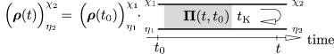
Figure 2: The density matrix evolves in time with the propagator $\bm{\Pi}$, which is a tensor of rank four.

In order to find the stationary density matrix for a system, which is described by a time-independent Hamiltonian, we consider the limit $t_{0}\rightarrow-\infty$. There is some characteristic time after which the system loses the information about its initial density matrix $\bm{\rho}_{\rm ini}=\lim_{t_{0}\rightarrow-\infty}\bm{\rho}(t_{0})$. We can, therefore, choose without loss of generality $\left(\bm{\rho}_{\rm ini}\right)^{\chi_{1}}_{\eta_{1}}=\delta_{\chi_{1},\chi_{0}}\delta_{\eta_{1},\chi_{0}}$ with an arbitrarily-picked state $\chi_{0}$, to get for the stationary (non-equilibrium) density matrix

$${\bigl{(}\bm{\rho}_{\rm st}\bigl{)}}_{\eta_{2}}^{\chi_{2}}=\lim_{t_{0}\rightarrow-\infty}{\Pi(t-t_{0})\vphantom{\bigl{)}}}_{\eta_{2}\chi_{0}}^{\chi_{2}\chi_{0}}\,,$$ (6)

independent of $\chi_{0}$. Here, for time-translation invariant systems, the propagator $\bm{\Pi}(t,t_{0})$ depends only on the difference of the time arguments $(t-t_{0})$. For the following, it is convenient to express the propagator in frequency representation $\bm{\Pi}(\omega)=\hbar^{-1}\int_{-\infty}^{0}dt\,\bm{\Pi}(-t)\,\exp[i(\omega-i0^{+})t]$. It can be constructed by the Dyson equation

$${\bm{\Pi}}(\omega) = {\bm{\Pi}}_{0}(\omega)+{\bm{\Pi}_{0}}(\omega){\bm{W}}(\omega){\bm{\Pi}}(\omega)$$ (7)

$$= \left[{{\bm{\Pi}}_{0}}^{-1}(\omega)-{\bm{W}}(\omega)\right]^{-1}\,.$$

The full propagator ${\bm{\Pi}}(\omega)$ depends on the free propagator ${\bm{\Pi}}_{0}(\omega)$ and the irreducible self energies $\bm{W}(\omega)$, which describes the influence of tunneling events between the dot and the leads. The Dyson equation is diagrammatically represented in Fig. 3. The frequency argument of the Laplace transformation appears in this diagrammatic languagediagrams as additional horizontal bosonic line transporting energy $\hbar\omega$.

Figure 3: Diagrammatical representation of the Dyson equation for the propagator. The self energy $\bm{W}$ sums up all irreducible tunnel diagrams. With $\bm{W}(\omega)$, we label the self energy, together with the parallel running frequency line $\omega$.

The free propagator (without tunneling) is given by

$${\Pi_{0}(\omega)}_{\eta_{2}\eta_{1}}^{\chi_{2}\chi_{1}}=\frac{i\delta_{\eta_{1}\eta_{2}}\delta_{\chi_{1}\chi_{2}}}{\varepsilon_{\eta_{1}}-\varepsilon_{\chi_{1}}-\hbar\omega+i0^{+}}\,,$$ (8)

where $\varepsilon_{\chi}$ ($\varepsilon_{\eta}$) is the energy of the dot state $\chi$ ($\eta$). Tunneling between the dot and the leads introduce the irreducible self energies $\bm{W}(\omega)$. We calculate $\bm{W}(\omega)$ in a perturbation expansion in the tunnel Hamiltonian Eq. (4). Each tunnel Hamiltonian generates one vertex (filled circle), on the Keldysh time contour $t_{\rm K}$, see Fig. 3. Since the leads are in equilibrium, their non-interacting fermionic degrees of freedom can be integrated out. Thereby two tunnel Hamiltonians each get contracted, symbolized by a line. Each line is associated with one tunnel event, transferring one particle and a frequency/energy from one vertex to the other. Therefore the lines have a defined direction and bear one order of the coupling constant $\Gamma=\Gamma_{\rm L}+\Gamma_{\rm R}$. We define the self energy $\bm{W}(\omega)$ as the sum of all irreducible tunnel diagrams (diagrams, which can not be cut at any real time, i.e. cut vertically, without cutting one tunneling line).

In Sec. III.4, we will then restrict our otherwise general calculation to the lowest-order expansion in $\Gamma$, i.e. we will include only diagrams with one tunnel line in $\bm{W}(\omega)$. A detailed description of how to calculate these lowest-order self energies as well as example calculations of $\bm{W}$ for the system under consideration can be found in Ref. braun1, .

To solve for the stationary density matrix ${\bm{\rho}}_{\rm st}$, we rewrite the Dyson Eq. (7) as $({\bm{\Pi}_{0}}(\omega)^{-1}-{\bm{W}}(\omega)){\bm{\Pi}}(\omega)=\bm{1}$, multiply both sides of the equation with $\omega$, use the final value theorem $\lim_{\omega\rightarrow 0}(i\hbar\omega+0^{+})\bm{\Pi}(\omega)=\lim_{t\rightarrow\infty}\bm{\Pi}(t)$, similar as for Laplace transformations, and employ Eq. (6), to get the generalized master equation

$$\bm{0}=\Bigl{[}\bm{\Pi}_{0}^{-1}(\omega=0)-{\bm{W}}(\omega=0)\Bigl{]}\,\,{\bm{\rho}}_{\rm st}$$ (9)

together with the normalization condition $\operatorname{Tr}[\bm{\rho}_{\rm st}]=1$.

The structure of Eq. (9) motivates the interpretation of the self energy $\bm{W}(\omega=0)$ as generalized transition rates. However, the self energy does not only describe real particle transfer between leads and dot, but it also accounts for tunneling-induced renormalization effects. It was shown in Refs. braun1, ; spincurrent, ; doubledot, ; Braig2005, , that these level renormalization effects may affect even the lowest-order contribution to the conductance. Therefore, a neglect of these renormalizations would break the consistancy of the lowest-order expansion in the tunnel coupling strength.bingdong ; RudzinskiBarnas ; gurvitz1 Recently, the frequency-dependent current noise of a quantum-dot spin valve structure was discussed in Ref. gurvitznoise, , in the limit of infinite bias voltage, where these level renormalizations can be neglected. One of the main advantages of the approach presented here is, that a rigid systematic computation of the generalized transition rates is possible, which include all renormalization effects. Therefore our approach is valid for arbitrary bias voltages.

III.2 Current

The current through barrier $r={\rm L},{\rm R}$ is defined as the change of charge $en_{r}=e\sum_{k\sigma}a^{{\dagger}}_{rk\sigma}a^{\,}_{rk\sigma}$ in lead $r$ due to tunneling, described by the operator

$$\hat{I}_{r}=e\frac{\partial n_{r}}{\partial t}=\frac{e}{i\hbar}[n_{r},H_{\rm T}]\,.$$ (10)

We define the operator for the current through the dot as $\hat{I}=(\hat{I}_{\rm L}-\hat{I}_{\rm R})/2$. Each term of the resulting current operator does contain a product of a lead and a dot operator. By integrating out the lead degrees of freedom, the current vertex (open circle) gets connected to a tunnel vertex by a contraction line as depicted in Fig. 4. Thereby the tunnel vertex can be either on the upper or lower time contour line.

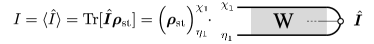
Figure 4: Diagrammatic representation of the current. By integrating out the lead degrees of freedom, the current vertex (open circle) gets contracted to one of the tunnel vertex in a self energy $\bm{W}(\omega=0)$.

To present a systematic way to calculate the current, we can utilize the close similarity of the tunnel Hamiltonian in Eq. (4) and the current operator in Eq. (10). Both differ only by the prefactor $e/\hbar$ and possibly by additional minus signs.

Following the work of Thielmann et al.,thielmann we define the object ${W^{I}}^{\chi_{1}\chi}_{\eta_{1}\eta}$ as the sums of all possible realizations of replacing one tunnel vertex (filled circle) by a current vertex (open circle) in the self energy ${W}^{\chi_{1}\chi}_{\eta_{1}\eta}$, compare Fig. 5. In technical terms, this means that each diagram is multiplied by a prefactor, determined by the position of the current vertex inside the diagram. If the current vertex is on the upper (lower) Keldysh time branch, and describes a particle tunneling into the right (left) lead or out of the left lead (right), multiply the diagram by $+1/2$, otherwise by $-1/2$. For clarity, we keep the factor $e/\hbar$ separate. For the detailed technical procedure of the replacement as well as the rules to construct and calculate the self energies, we refer to Ref. thielmann, . The average of one current operator, i.e. the $dc-$current flowing through the system is then given by

$$I=\langle\hat{I}\rangle=\frac{e}{2\hbar}\operatorname{Tr}[{\bm{W}}^{I}(\omega=0)\,{\bm{\rho}}_{\rm st}]\,.$$ (11)

The trace selects the diagonal matrix elements, which regards that the Keldysh line must be closed at the end of the diagram, see Fig. 5, requiring that the dot state of the upper and lower time branch match.

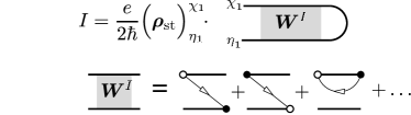
Figure 5: Reformulation of the current as function of $\bm{W}^{I}(\omega=0)$, the self energy with one tunnel vertex replaced by a current vertex.

To see, that the diagrams in Fig. 4 and Fig. 5 are equal, one must consider, that all diagrams, where the rightmost vertex is a tunnel vertex will cancel each other when performing the trace. This happens, since by moving the rightmost tunnel vertex from the upper (lower) to the lower (upper) Keldysh time line, the diagram aquires only a minus sign.diagrams

III.3 Current-current correlation

We define the frequency-dependent noise as the Fourier transform of $S(t)=\langle\hat{I}(t)\hat{I}(0)\rangle+\langle\hat{I}(0)\hat{I}(t)\rangle-2\langle\hat{I}\rangle^{2}$, which can be written as

$$S(\omega) = \int^{\infty}_{0}\!\!\!\!\!dt\Bigl{(}\langle\hat{I}(t)\hat{I}(0)\rangle+\langle\hat{I}(0)\hat{I}(t)\rangle\Bigl{)}\Bigl{(}e^{-i\omega t}+e^{+i\omega t}\Bigl{)}$$ (12)

$$-4\pi\,\delta(\omega)\,\langle\hat{I}\rangle^{2}\,.$$

We restrict our discussion to the above defined symmetrized and, therefore, real noise since it can be measured by a classical detector.quantummeasuremnet The unsymmetrized noise would have an additional complex component, describing absorption and emission processes,assymmetric that depend on the specifics of the detector.

Since the dot-lead interface capacitances are much less sensitive to the contact geometry than the tunnel couplings $\Gamma_{\rm L/R}$, we assume an equal capacitance of the left and right interface, while still allowing for different tunnel-coupling strengths. Following the Ramon-Shockleytheorem theorem, we have then to define current operator also symmetrized with respect to the left and right interface as already done in Sec. III.2.

The diagrammatic calculation of the current-current correlation function is now straightforward. Instead of replacing one tunnel vertex by a current vertex on the Keldysh time contour, as for the average current, one must replace two vertices. The additional frequency $\omega$ of the Fourier transformation in Eq. (12) can be incorporated in the diagrams as an additional bosonic energy line (dashed) running from $t$ to $0$, i.e. between the two current vertices.johansson This line must not be confused with a tunnel line, since it only transfers energy $\hbar\omega$, and no particle. By introducing the self energy $\bm{W}$ all diagrams of the current-current correlation function can be grouped in two different classesjohansson ; thielmann as shown in Fig. 6. Either both current vertices are incorporated in the same irreducible block diagram, or into two different ones that are separated by the propagator $\bm{\Pi}(\omega)$.

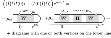
Figure 6: Regrouping of the noise expansion by introducing the irreducible self energy $\bm{W}$, and the propagator $\bm{\Pi}(\omega)$.

The order of the current operator on the Keldysh contour is determined by its ordering in the correlator, so the current operator at time $0$ lies on the upper branch for $\langle\hat{I}(t)\hat{I}(0)\rangle$ and on the lower branch for $\langle\hat{I}(0)\hat{I}(t)\rangle$. Since in Eq. (12) we defined the noise symmetrized with respect to the operator ordering, we just allow every combination of current vertex replacements in the $\bm{W}$’s. This includes also diagrams where one or both vertices are located on the lower time contour (this type of diagrams are not explicitly drawn in Fig. 6).

By including the current vertices and the frequency line in the self energies, three variants of the self energy ${\bm{W}}$ are generated. The objects ${\bm{W}}^{I}_{>}(\omega)$ and ${\bm{W}}^{I}_{<}(\omega)$ are the sum of all irreducible diagrams, where one tunnel vertex is replaced by a current vertex in any topological different way. The subindex $>(<)$ indicates, that the frequency line connected to the current vertex leaves or enters the diagram to the right (left) side. In the zero-frequency limit, the two objects become equal ${\bm{W}}^{I}_{>}(\omega=0)={\bm{W}}^{I}_{<}(\omega=0)\equiv{\bm{W}}^{I}$.

The third object ${\bm{W}}^{II}(\omega)$ sums irreducible diagrams with two tunnel vertices replaced each by a current vertex in any topological different way. The current vertices are connected by the frequency line $\omega$. The diagrammatical picture of the objects ${\bm{W}}(\omega)$, ${\bm{W}}^{II}(\omega)$, ${\bm{W}}^{I}_{>}(\omega)$, and ${\bm{W}}^{I}_{<}(\omega)$ are shown in Fig. 7.

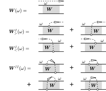
Figure 7: Different variations of the self energy $\bm{W}$.

With these definitions the diagrams for the frequency-dependent noise in Fig. 6 can be directly translated into the formula

$$S(\omega) = \frac{e^{2}}{2\hbar}\operatorname{Tr}[{\bm{W}}^{II}(\omega){\bm{\rho}}_{\rm st}+{\bm{W}}^{I}_{<}(\omega)\,{\bm{\Pi}}(\omega)\,{\bm{W}}^{I}_{>}(\omega){\bm{\rho}}_{\rm st}]$$ (13)

$$-2\pi\delta(\omega)\,\langle\hat{I}\rangle^{2}+(\omega\rightarrow-\omega)\,.$$

We remark that the first line in Eq. (13) diverges as $\omega\rightarrow 0$. While the $\bm{W}$’s are regular for $\omega\rightarrow 0$, the propagator ${\bm{\Pi}}(\omega)$ goes as $i/(-\hbar\omega+i0^{+})$ times $\bm{\Pi}(t\rightarrow\infty)$, which is related to ${\bm{\rho}}_{\rm st}$ via Eq. (6). In the limit $\omega\rightarrow 0$ the propagator therefore yields both a delta function $\delta(\omega)$ and a $1/\omega$ divergence. For the full expression of the noise, these divergences are canceled by the delta-function term in the second line of Eq. (13) and by the terms with $\omega\rightarrow-\omega$, respectively. As a consequence, $S(\omega)$ remains regular also in the limit $\omega\rightarrow 0$.

III.4 Low-frequency noise in the sequential-tunnel limit

Equation (13) is the general expression for the frequency-dependent current noise. In the following paper, we consider only the limit of weak dot-lead tunnel coupling, $\Gamma\ll k_{\rm B}T$, and therefore include only diagrams with at most one tunnel line in the $\bm{W}$’s. However, this procedure is not a consistent expansion scheme for the noise $S(\omega)$ itself. By expanding the $\bm{W}$’s up to linear order in $\Gamma$, the result of Eq. (13) is the consistent noise linear in $\Gamma$ plus some higher-order contributions proportional to $\Gamma^{2}$. Since co-tunnel processes also give rise to quadratic contributions, we have to discard these terms as long as we neglect the quadratic cotunnel contributions of $\bm{W}$. If one is interested in the noise up to second order in $\Gamma$, then these higher-order terms generated by lower-order $\bm{W}$’s are of course an essential part of the result.thielmann2

Further, we are looking for signatures of the internal charge and spin dynamics of the quantum-dot in the frequency-dependent current noise. Therefore - if we neglect external magnetic fields at this point - we concentrate on frequencies that are at most of the same order of the tunnel coupling $\Gamma$. If we limit the range in which we want to calculate the current noise to $\hbar\omega\lesssim\Gamma$, we can neglect the frequency dependence of the $\bm{W}$’s. Each correction of the $\bm{W}$’s would scale at least with $\omega\Gamma\approx\Gamma^{2}$, making them as important as the neglected co-tunnel processes.

The neglect of the terms in $\bm{W}$ which are at least linear in frequency has two main advantages. First, it considerably simplifies the calculation of the $\bm{W}$’s. Second, it automatically removes the quadratic parts of the noise, so Eq. (13) gives a result consistent in linear order in $\Gamma$. In this low-frequency limit, the noise can then be written as

$$S(\omega) = \frac{e^{2}}{\hbar}\operatorname{Tr}[{\bm{W}}^{II}{\bm{\rho}}_{\rm st}+{\bm{W}}^{I}\,\Bigl{[}{\bm{\Pi}}_{0}^{-1}(\omega)-{\bm{W}}\Bigl{]}^{-1}\,{\bm{W}}^{I}{\bm{\rho}}_{\rm st}]$$ (14)

$$-2\pi\delta(\omega)\,\langle\hat{I}\rangle^{2}+(\omega\rightarrow-\omega)$$

where $\bm{W}^{I}\equiv{\bm{W}}^{I}_{>}(\omega=0)={\bm{W}}^{I}_{<}(\omega=0)$, ${\bm{W}}\equiv{\bm{W}}(\omega=0)$, and ${\bm{W}}^{II}\equiv{\bm{W}}^{II}(\omega=0)$. This means, that the bosonic frequency lines $\omega$ in the diagrams as shown in Fig. 7 can be neglected. The only remaining frequency-dependent part is the free propagator ${\bm{\Pi}}_{0}(\omega)$.

This formalism, of course, reproduces the noise spectrum of a single-level quantum dot connected to normal leads as known from literature.review If one can approximate the Fermi functions by one or zero only, i.e. if the dot levels are away from the Fermi edges of the leads the Fano factor shows a Lorentzian dependence on the noise frequency $\omega$

$$F(\omega) \equiv \frac{S(\omega)}{2eI}=\frac{1}{2}+\frac{(2\Gamma_{\rm L}-\Gamma_{\rm R})^{2}}{(2\Gamma_{\rm L}+\Gamma_{\rm R})^{2}+(\hbar\omega)^{2}}\qquad$$ (15)

for a bias voltage allowing only an empty or singly-occupied dot, and

$$F(\omega) = \frac{1}{2}+\frac{(\Gamma_{\rm L}-\Gamma_{\rm R})^{2}}{(\Gamma_{\rm L}+\Gamma_{\rm R})^{2}+(\hbar\omega)^{2}}$$ (16)

for higher bias voltages, when double occupation is also allowed.

III.5 Technical summary

The technical scheme for calculating the zero- and low-frequency current noise is the following: First the objects $\bm{W}$, $\bm{W}^{I}$ and $\bm{W}^{II}$ must be calculated in the $\omega=0$ limit, using the diagrammatic approach, see Ref. braun1, .

In the next step, we calculate the reduced density matrix $\bm{\rho}$ of a single-level quantum dot, which is a $4\times 4$ matrix,

$${\bm{\rho}}=\left(\begin{array}[]{cccc}\rho_{0}^{0}&0&0&0\\ 0&\rho_{\uparrow}^{\uparrow}&\,\rho^{\uparrow}_{\downarrow}&0\\ 0&\,\rho^{\downarrow}_{\uparrow}&\rho_{\downarrow}^{\downarrow}&0\\ 0&0&0&\rho_{\rm d}^{\rm d}\end{array}\right)\,,$$ (21)

since the dot can be either empty ($\chi=0$), occupied with a spin-up ($\chi=\uparrow$) or a spin-down ($\chi=\downarrow$) electron, or doubly occupied ($\chi=\rm d$). The diagonal elements of the matrix can be interpreted as the probability to find the dot in the respective state, while the inner $2\times 2$ matrix is the $SU(2)$ representation of the average spin on the dot. All off-diagonal elements connecting different charge states are prohibited by charge conservation.

For technical reasons it is convenient, to express the density matrix as vector: $\rho_{\rm st}=(P_{0}^{0},P_{\uparrow}^{\uparrow},P_{\downarrow}^{\downarrow},P_{\rm d}^{\rm d},P^{\uparrow}_{\downarrow},P^{\downarrow}_{\uparrow})^{T}$. Then the forth-order tensors $\bm{W}$’s and $\bm{\Pi}(\omega)$’s are only $6\times 6$ matrices, see App. A, and standard computer implemented matrix operations can be used. It is worth to point out, that in the vector notation, the trace for example in Eq. (14) is then not the sum of all elements of the resulting vector as assumed by Ref. bingdong, , but only the sum of the first four entries. These elements correspond to the diagonal entries of the final density matrix. In the notation of Ref. thielmann, , this can be achieved by the vector $e^{T}=(1,1,1,1,0,0)$.

The stationary density matrix follows from the master Eq. (9) $\,0=-i(\varepsilon_{\eta}-\varepsilon_{\chi})(\rho_{st})^{\chi}_{\eta}+\sum_{\chi_{1},\eta_{1}}W^{\chi\chi_{1}}_{\eta\eta_{1}}(\rho_{st})^{\chi_{1}}_{\eta_{1}}\,$ under the constraint of probability normalization $e^{T}\cdot\rho_{\rm st}=1$. The average $dc-$current through the system is given by $I=e/(2\hbar)e^{T}\cdot{\bm{W}^{I}}\cdot\rho_{\rm st}$. In the low-frequency limit the frequency-dependent propagator $\bm{\Pi}(\omega)$ can be constructed from the frequency-dependent free propagator $\bm{\Pi}_{0}(\omega)$ and the frequency-independent self energy $\bm{W}(\omega=0)$. The low-frequency noise is then given by the matrix multiplication $S(\omega)=e^{2}/(2\hbar)e^{T}\cdot({\bm{W}^{II}+\bm{W}^{I}\bm{\Pi}(\omega)\bm{W}^{I}})\cdot\rho_{\rm st}+(\omega\rightarrow-\omega)$, where the $i0^{+}$ in the denominator of the propagator is dropped, since the term arising from the $i0^{+}$ contribution cancels the delta function in Eq. (13).

IV Results

In this section, we discuss our results for zero- and finite-frequency current noise in a quantum dot connected to ferromagnetic leads with non-collinear magnetizations. The relative energies of a single-level dot is sketched in Fig. 8.

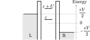
Figure 8: Sketch of different energies involved. Since we assume equal tunnel interface capacities, the voltage drop on the left and right side is symmetric.

We always assume $k_{\rm B}T\gg\Gamma$, and that the single-particle state is above the equilibrium Fermi energy of the leads, otherwise higher-order tunnel processes could become important.thielmann2 ; superpoissonian2 ; assymmetric ; Weymann

IV.1 Zero-frequency noise

We start our discussion with the zero-frequency noise. In Fig. 9, we plot results for $F(\omega\rightarrow 0)=S(\omega\rightarrow 0)/(2eI)$, i.e. the zero-frequency Fano factor for the quantum dot contacted by ferromagnetic leads. In Fig. 9a), the leads are aligned parallel. For $eV/2<\varepsilon$, when the dot level is above the lead Fermi energies, the dot is predominantly empty, and interaction effects are negligible leading to a Fano factor of $1$. In the voltage window $\varepsilon<eV/2<\varepsilon+U$, when the dot can only be empty or singly occupied, we can observe super-Poissonian noise due to dynamical spin blockadecottet ; superpoissonian2 ; Bulka1999 for sufficiently high lead polarization. The minority spins have a much longer dwell time inside the dot than the majority spins. In this way, they effectively chop the current leading to bunches of majority spins. While the current in this regime $I=2\Gamma_{\rm L}\Gamma_{\rm R}/(2\Gamma_{\rm L}+\Gamma_{\rm R})$ does not depend on the polarization $p$ of the leads, the Fano factor

$$F(0)=\frac{4\frac{1+p^{2}}{1-p^{2}}\Gamma_{\rm L}^{2}+\Gamma_{\rm R}^{2}}{(2\Gamma_{\rm L}+\Gamma_{\rm R})^{2}}$$ (22)

even diverges for $p\rightarrow 1$. If the voltage exceeds the value necessary to occupy the dot with two electrons ($eV/2>\varepsilon+U$), the noise is no longer sensitive to a lead polarization.

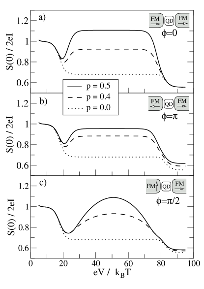
Figure 9: Zero-frequency current noise through a quantum dot spin valve. In panel a), the lead magnetizations are aligned parallel, in panel b) anti-parallel, and in panel c) the lead magnetizations enclose an angle of $\pi/2$. The different lines correspond to different values of the lead polarization $p$. Other parameters are $\varepsilon=10k_{\rm B}T$, $U=30k_{\rm B}T$, and $\Gamma_{\rm L}=2\Gamma_{\rm R}$

Also in the case of anti-parallel aligned leads, the Fano factor rises in the voltage regime $\varepsilon<eV/2<\varepsilon+U$ as seen in Fig. 9b). The dot is primarily occupied with an electron with majority spin of the source lead, i.e. minority spin for the drain lead, since this spin has the longest dwell time. If the electron tunnels to the drain lead, it gets predominantly replaced by a majority spin of the source lead. For a high enough lead polarization, only one spin component becomes important. Further this spin component is strongly coupled to the source lead and weakly coupling to the drain lead, therefore the Fano factor approaches unity.

If the leads are non-collinearly aligned, for example enclose an angle $\phi=\pi/2$ in Fig. 9c), a qualitatively different behavior can be observed. Now, the typical Coulomb plateaus are modulated. This shape arises, since the dot spin starts to precess around the lead magnetizations. The tunnel coupling between the ferromagnetic lead $r=$L/R and the dot induces the exchange field contributionbraun1 ; braun2

$${\bm{B}}_{r}=p\,\frac{\Gamma_{r}{\bf\hat{n}}_{r}}{\pi\hbar}\int^{\prime}d\omega\left(\frac{f_{r}(\omega)}{\omega-\varepsilon-U}+\frac{1-f_{r}(\omega)}{\omega-\varepsilon}\right)\,,$$ (23)

generating an intrinsic spin precession of the dot spin around the lead magnetizations. This exchange field automatically appears in a rigid calculation of the generalized transition rates $\bm{W}$.

The intrinsic spin precession due to the exchange field counteracts the dynamical spin blockade. The exchange coupling to one lead is maximal, if its Fermi energy coincides with the dot energy levels, i.e. the coupling to the source lead is maximal at the voltages $eV/2=\varepsilon$ and $eV/2=\varepsilon+U$ and changes its sign in between. Therefore the reduction of the Fano factor is non-monotonic, and so is the variation of the Coulomb plateaus. It is worth to point out, that to observe this spin precession mechanism in the conductance of the device a relatively high spin polarization of the leads is required. But the noise is much more sensitive to this effect than the conductance, that a polarization as expected for Fe, Co, or Nipasupathy is well sufficient.

The zero-frequency Fano factor as a function of the angle $\phi$ between the two lead magnetization vectors is plotted in Fig. 10. The black lines are for the bias voltage $eV=50k_{\rm B}T$, where the exchange field influence is weak, while the gray lines is for the bias voltage $eV=30k_{\rm B}T$. Since both voltages are within the voltage window allowing only single occupation of the dot, compare Fig. 9, the tunnel rates do not change significantly within this voltage range. Only the exchange field varies with voltage. Since the exchange field suppresses bunching due to spin precession, the black and gray curves split.

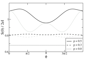
Figure 10: Fano factor of a quantum dot spin valve as a function of the angle $\phi$, enclosed by the lead magnetizations. The black lines are for a bias voltage $eV=50k_{\rm B}T$, where the exchange field is very weak, while the gray curves are for $eV=30k_{\rm B}T$, where the exchange field is more pronounced. Further parameters are $\varepsilon=10k_{\rm B}T$, $U=30k_{\rm B}T$, and $\Gamma_{\rm L}=2\Gamma_{\rm R}$

For $\phi=0$ and $\phi=\pi$ the accumulated spin is collinearly aligned with the exchange field, and no spin precession arises.

IV.2 Finite-frequency noise and weak magnetic fields

The $dc-$conductance of the quantum-dot spin valve is a direct measure of the time-averaged spin in the dot. On the other side, the power spectrum of the current noise can also measure the time-dependent dynamics of the individual electron spins in the dot. The spin precesses in the exchange field as well as an external magnetic field. This gives rise to a signal in the frequency-dependent noise at the Larmor frequency of the total field.

By including an external magnetic field in the noise calculation, one has to distinguish two different parameter regimes: either the Zeeman splitting $\Delta\equiv g\mu_{\rm B}B_{\rm ext}$ is of the same order of magnitude as the level broadening $\Delta\approx\Gamma_{\rm L},\Gamma_{\rm R}$, or it significantly exceeds the tunnel coupling $\Delta\gg\Gamma_{\rm L},\Gamma_{\rm R}$. In this section we focus on the first case, while the latter case is treated in Sec. IV.3.

By choosing the spin-quantization axis of the dot subsystem parallel to the external magnetic field, the magnetic field only induces a Zeeman splitting of the single-particle level $\varepsilon$ in $\varepsilon_{\uparrow}=\varepsilon+\Delta/2$ and $\varepsilon_{\downarrow}=\varepsilon-\Delta/2$. Since $\Delta\approx\Gamma_{\rm L},\Gamma_{\rm R}$, we can expand the $\bm{W}$’s also in $\Delta$ and keep only the zeroth-order terms, since each correction of the self energies would be proportional to $\Delta\cdot\Gamma\approx\Gamma^{2}$. The Zeeman splitting must only be considered for the free propagator. With Eq. (8), the propagator is then given by

$$\bm{\Pi}_{0}(\omega)=i\left(\begin{array}[]{cccccc}\omega&0&0&0&0&0\\ 0&\omega&0&0&0&0\\ 0&0&\omega&0&0&0\\ 0&0&0&\omega&0&0\\ 0&0&0&0&\omega+\Delta&0\\ 0&0&0&0&0&\omega-\Delta\end{array}\right)^{-1}\,,\,\,\,\,$$ (30)

where we already dropped the $+i0^{+}$ in the denominator, and use the matrix notation as introduced in Sec. III.5. The two last rows of this matrix govern the time evolution of $\rho_{\uparrow}^{\downarrow}$ and $\rho^{\uparrow}_{\downarrow}$, representing the spin components transverse to the quantization axis, i.e. transverse to the applied magnetic field. The change of the denominator by the Zeeman energy $\Delta$ describes just the precession movement of the transverse spin component. Since the free propagator $\bm{\Pi}_{0}(\omega)$ is a function of $\Delta$, the Zeeman energy modifies the full propagator $\bm{\Pi}(\omega)$ as well as the (zeroth-order) stationary density matrix $\bm{\rho}_{\rm st}$, via the master Eq. (9).

The numerical results are plotted in Fig. 11 and Fig. 12. In Fig. 11 the magnetizations of the leads are aligned parallel, and a magnetic field is applied perpendicular to the lead magnetizations. With parallel aligned leads and equal polarizations in both leads, no average spin accumulates on the dot, and therefore the current-voltage characteristic as shown in the inset of Fig. 11, shows neither magnetoresistance nor the Hanle effect if a transverse magnetic field is applied.braun2 In contrast to the conductance, which depends on the average dot spin only, the frequency-dependent noise is sensitive to the time-dependent dynamics of the spin on the dot. Therefore the field-induced spin precession is visible in the noise power spectrum. For $B=0$ the Fano factor shows a Lorentzian dependence of the noise frequency. Thereby the Fano factor exceeds unity due to the bunching effect, as discussed in Sec. IV.1.

With increasing magnetic field, spin precession lifts the dynamical spin blockade inside the dot, and the Fano factor decreases at $\omega\approx 0$.

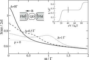
Figure 11: Frequency-dependent Fano factor of a quantum dot connected to parallel aligned leads for various perpendicular applied external magnetic fields. The parameters are $p=0.5$, $\varepsilon=10k_{\rm B}T$, $U=30k_{\rm B}T$, $eV=40k_{\rm B}T$ and $\Gamma_{\rm L}=2\Gamma_{\rm R}$. The inset shows the current bias-voltage characteristic, which does not depend on the applied magnetic field.

Further a resonance line evolves approximatively at the Larmor frequency of the applied magnetic field. The line width of the resonance is given by the damping due to tunnel events. If the dot can only be singly occupied, the damping coefficient equals the tunnel-out rate $\Gamma_{\rm R}$, if the dot can also be doubly occupied, also tunnel-in events contribute.

The deviation of the resonance line position from the Larmor frequency, one would expect by considering the applied magnetic field only, is caused by the exchange interaction. The spin inside the dot precesses in the total field containing the external magnetic field and the exchange field.braun1 Dependent on their relative orientation, the exchange field can increase or decrease the total field strength.

Since the exchange field is a function of the applied bias voltage, the resonance peak is shifted by changing the bias voltage. In Fig. 12, the finite frequency noise for a quantum dot is plotted, where the lead’s magnetizations enclose an angle $\phi=\pi/2$, i.e. their magnetizations are perpendicular to each other. Further an external magnetic field is applied parallel to the source lead magnetization. The exchange fields originating from the leads has to be added to the external field. By varying the bias voltage (without significantly changing the transition rates, as indicated in the inset of Fig. 12) the exchange field varies, and the position of the resonance peak is shifted.

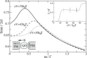
Figure 12: The Fano factor of a quantum dot spin valve as a function of the noise frequency. The lead magnetizations enclose an angle $\phi=\pi/2$ and an external magnetic field $g\mu_{\rm B}B_{\rm ext}=1/2\Gamma$ is applied parallel to the source lead magnetization. The vertical gray line marks the Larmor frequency given by the external magnetic field only. For the three different bias voltages, $eV=30k_{\rm B}T$ (dot-dot-dashed), $eV=45k_{\rm B}T$ (dashed) and $eV=70k_{\rm B}T$ (solid), the strength of the exchange field varies, and so does the position of the resonance peak. Other system parameters are $p=0.5$, $\varepsilon=10k_{\rm B}T$, $U=30k_{\rm B}T$, and $\Gamma_{\rm L}=2\Gamma_{\rm R}$

IV.3 Limit of strong magnetic fields

In this section, we discuss the case of an applied magnetic field, where the Zeeman energy $\Delta\equiv g\mu_{\rm B}B_{\rm ext}\gg\Gamma_{\rm L},\Gamma_{\rm R}$ exceeds the tunnel coupling strength. As a simplification, we can consider the tunnel rates (i.e. the $\bm{W}$’s) still as independent of $\Delta$ as well as of $\omega$. This assumption is justified, if the distance between the quantum dot states and lead Fermi surfaces well exceeds temperature $k_{\rm B}T$, the Zeeman splitting $\Delta$ and the noise frequency $\hbar\omega$.

For a clear analytic expressions, we expand the stationary density matrix in zeroth order in $\Gamma/\Delta$. Further we consider only the noise frequency range $\omega=\Delta\pm\Gamma$. In this regime the first five diagonal entries of the free propagator in Eq. (30) can be treated as zeroth order in $\Gamma$, i.e. their contribution drops out for the lowest-order noise, only the last entry $1/(\omega-\Delta)\approx 1/\Gamma$ is kept. This considerably simplifies the calculation, since all bunching effects and the exchange field components perpendicular to the external field can be neglected.

Let us consider a single-level quantum dot with such an applied voltage, where approximately $f_{\rm L}(\varepsilon)=1$ and $f_{\rm L}(\varepsilon+U)=f_{\rm R}(\varepsilon)=f_{\rm R}(\varepsilon+U)=0$, i.e. the applied bias voltage allows only an empty or singly-occupied dot. For an external applied magnetic field perpendicular to both lead magnetizations $\bm{B}_{\rm ext}\perp\hat{\bm{n}}_{\rm L},\hat{\bm{n}}_{\rm R}$ the Fano factor

$$F(\omega)=\frac{1}{2}+\frac{p^{2}}{4}\,\frac{\Gamma_{\rm R}^{2}\cos\phi\,\,+\,\,\Gamma_{\rm R}(\omega-\Delta)\sin\phi}{\Gamma_{\rm R}^{2}+(\omega-\Delta)^{2}}\,$$ (31)

shows a resonance signal at the Larmor frequency $\hbar\omega=\Delta$. By representing the frequency-dependent Fano factor as an integral over time,

$$F(\omega)=\frac{1}{2}+\frac{\Gamma_{\rm R}p^{2}}{4\hbar}\,\Re\int_{0}^{\infty}\!\!\!\!dt\,\,e^{-\Gamma_{\rm R}/\hbar\cdot t}\,\,e^{-i(\Delta/\hbar\cdot t-\phi)}\,\,e^{i\omega t}\,,\quad$$ (32)

the discussion of the functional form becomes more transparent. At $t=0$ an electron tunnels from the source (left) lead in the dot. This electron decays on average to the drain (right) lead on the time scale $\hbar/\Gamma_{\rm R}$. During its dwell time the electron precesses inside the dot with the Larmor frequency $\Delta/\hbar$. This precession modulates the decay rate, due to magnetoresistance effects. The tunnel-out event is more likely, if the spin is aligned parallel to the drain lead magnetization than if anti-parallel aligned. The phase of this modulation is given by the relative angle of the lead magnetizations, and the effect can give rise to an absorption or dispersion line shape, see Fig. 13.

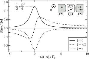
Figure 13: Fano factor as a function of noise frequency for different angles $\phi$ in the frequency range of the Larmor frequency. The applied voltage does only allow single occupation of the dot. Other system parameters are as in Fig. 12.

By shifting the gate voltage such that $f_{\rm L}(\varepsilon)=f_{\rm L}(\varepsilon+U)=f_{\rm R}(\varepsilon)=1$ and $f_{\rm R}(\varepsilon+U)=0$, the dot will always be at least occupied by one electron. Then the noise shows the same resonance, only $\Gamma_{\rm R}$ and $\phi$ must be replaced by $\Gamma_{\rm L}$ and $-\phi$.

If the leads are aligned parallel, the electron will leave the dot primary directly after the tunnel-in event, or after one revolution, i.e. the decay is modulated with a cosine function. If the leads are aligned perpendicular to each other, then the electron must be rotated by the angle $\pi/2$ (or $3\pi/2$) before the maximum probability for the tunneling-out event is reached. The decay is then modulated by a (minus) sine function.

The phase dependence of the noise resonance is also predicted for a double-dot system.bingdong ; gurvitz2 Let us consider two dots connected in series, see Fig. 14A), and an electron from the left (source) electrode enters the left dot. Since this is not an eigenstate of the isolated double-dot system, the electron coherently oscillates between the two dots with the frequency $\omega_{\rm R}$. After the time $t=\pi/\omega_{\rm R}$, the electron is in the right dot and can tunnel to the drain lead. This corresponds to the $\phi=\pi$ case resulting a dip in the noise. The realization of the $\phi=0$ case would be a double dot where the left (source) and right (drain) lead is contacted to the same dot, see Fig. 14B). Here the electron must stay a multiple of $2\pi/\omega_{\rm R}$ inside the double dot to tunnel to the drain lead, giving a peak in the frequency noise spectrum. Other values of $\phi$ have no double-dot-system analogon.

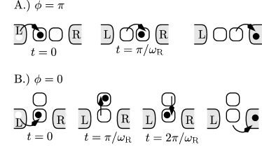
Figure 14: The double dot analog for the decay phase shift $\phi=0$ and $\phi=\pi$ of the electrons.

IV.4 Influence of spin relaxation

The density matrix approach offers a way to phenomenologically include spin relaxation by supplementing the matrix $\bm{W}$ by

$$\bm{W}^{\prime}=\bm{W}+\hbar\left(\begin{array}[]{cccccc}0&0&0&0&0&0\\ 0&-\frac{1}{T_{1}}&+\frac{1}{T_{1}}&0&0&0\\ 0&+\frac{1}{T_{1}}&-\frac{1}{T_{1}}&0&0&0\\ 0&0&0&0&0&0\\ 0&0&0&0&-\frac{1}{T_{2}}&0\\ 0&0&0&0&0&-\frac{1}{T_{2}}\end{array}\right)\,.\,$$ (39)

The entries in the lower right corner of Eq. (39) describe the exponential decay of the transverse spin components on the time scale $T_{2}$, and the block in the upper left corner describes an equilibration of the occupation probability for spin up and down. If one define the average spin vector on the quantum dot by $\bm{S}=(\rho^{\uparrow}_{\downarrow}+\rho^{\downarrow}_{\uparrow},i\rho^{\uparrow}_{\downarrow}-i\rho_{\uparrow}^{\downarrow},\rho_{\uparrow}^{\uparrow}-\rho^{\downarrow}_{\downarrow})/2$ the master Eq. (9) becomes a Bloch equation.braun1 The new term in Eq. (39) introduces an additional exponential decay term in this Bloch equation. In the limit of weak Zeeman splitting as discussed throughout the paper, $T_{1}$ and $T_{2}$ become equal, and $\bm{W}^{\prime}$ includes an isotropic exponential damping of the spin on the dot. Thereby the master equation describing the change of the probability $\partial_{t}(P_{\uparrow}^{\uparrow}+P_{\downarrow}^{\downarrow})$ for single occupation is not affected by this relaxation term.

The modified rate matrix $\bm{W}^{\prime}$ enters the noise calculation via the calculation of the stationary density matrix and via the propagator $\bm{\Pi}(\omega)$. The numerical solution for the case of parallel aligned lead magnetizations is plotted in Fig. 15.

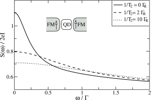
Figure 15: Frequency dependence of the Fano factor if the leads are aligned parallel. With increasing spin relaxation, the spin blockade and therefore the bunching effect is reduced. Other system parameters are as in Fig. 11.

With increasing the spin decoherence, the spin related effects decrease, which is the expected behavior for spin-decoherence. To completely suppress the spin related effects the spin life time must significantly exceed the inverse tunnel coupling, i.e. the spin related effects are not very fragile against spin-decoherence.

Several articlesRudzinskiBarnas ; SouzaEguesJauho ; bingdong try to model spin relaxation by the Hamiltonian $H_{\rm rel}=Rc^{\dagger}_{\uparrow}c_{\downarrow}+R^{\star}c^{\dagger}_{\downarrow}c_{\uparrow}\,,$ which is from the physical point of view dissatisfying, since it does not describe incoherent relaxation processes but coherent precession in a transverse magnetic field.QM1 This ansatz leads to a completely different behavior of the frequency-dependent current noise. Instead of a suppression of all spin-related effects with increasing the parameter $R$, as expected for spin relaxation, an external field generates a resonance line. With increasing the field strength, this line just shifts to higher and higher frequencies, but does not vanish.

V Conclusions

By contacting a quantum dot to ferromagnetic leads, the transport characteristic through the device crucially depends on the quantum-dot spin. In this paper we discussed the influence of the spin precession of the dot electron in the tunnel-induced exchange field and an applied external magnetic field. While the conductance depends only on the time-average dot spin, the current-current correlation function is sensitive to its time-dependent evolution.

In the zero-frequency limit, the spin precession lift the dynamical spin blockade, and therefore reduce the zero-frequency noise. At the Larmor frequency, corresponding to the sum of exchange and applied field, the single-spin precession leads to a resonance in the frequency dependent current-current correlation function. Responsible for the resonance is the tunnel-out process of a dot electron to the drain lead. Due to magnetoresistance, the tunnel probability depend on the relative angle of dot spin and drain magnetization. Therefore the spin precession leads to an oscillation of the tunnel probability, visible in the current-current correlation function. The shape of the resonance in the current-current correlation can either have an absorption or dispersion lineshape, depending on the relative angle between the lead magnetizations.

Finally, we show how to properly include spin decoherence, and discuss why modelling spin relaxation by an external field transverse to the spin quantization axis, as done sometimes in the literature, is unsatisfying.

Appendix A Generalized transition rates

The generalized transition matrix $\bm{W}$ is given by the solution of the self energy diagrams up to linear order in the coupling strength $\Gamma$. We have choosen the quantization axis perpendicular to both lead magnetizations, and the $x-$axis symmetric with respect to the magnetizations. Arranged in the matrix notation introduced in Sec. III.5 we get

$$\bm{W}\bigl{|}_{\omega=0}=\Gamma_{\rm L}\,{\bf A}_{\rm L}+({\rm L}\rightarrow{\rm R})\,,\qquad$$ (40)

with the matrix $\bm{A}_{\rm L}$ given by

$$\left(\begin{array}[]{cccccc}-2f^{+}_{\rm L}(\varepsilon)&f^{-}_{\rm L}(\varepsilon)&f^{-}_{\rm L}(\varepsilon)&0&pf^{-}_{\rm L}(\varepsilon)\,e^{i\phi_{\rm L}}&pf^{-}_{\rm L}(\varepsilon)e^{-i\phi_{\rm L}}\\ f^{+}_{\rm L}(\varepsilon)&-y_{\rm L}&0&f^{-}_{\rm L}(\varepsilon+U)&-\frac{p}{2}(x_{\rm L}-iB_{\rm L})e^{i\phi_{\rm L}}&-\frac{p}{2}(x_{\rm L}+iB_{\rm L})e^{-i\phi_{\rm L}}\\ f^{+}_{\rm L}(\varepsilon)&0&-y_{\rm L}&f^{-}_{\rm L}(\varepsilon+U)&-\frac{p}{2}(x_{\rm L}+iB_{\rm L})e^{i\phi_{\rm L}}&-\frac{p}{2}(x_{\rm L}-iB_{\rm L})e^{-i\phi_{\rm L}}\\ 0&f^{+}_{\rm L}(\varepsilon+U)&f^{+}_{\rm L}(\varepsilon+U)&-2f^{-}_{\rm L}(\varepsilon+U)&-pf^{+}_{\rm L}(\varepsilon+U)\,e^{i\phi_{\rm L}}&-pf^{+}_{\rm L}(\varepsilon+U)e^{-i\phi_{\rm L}}\\ pf^{+}_{\rm L}(\varepsilon)e^{-i\phi_{\rm L}}&-\frac{p}{2}(x_{\rm L}-iB_{\rm L})e^{-i\phi_{\rm L}}&-\frac{p}{2}(x_{\rm L}+iB_{\rm L})e^{-i\phi_{\rm L}}&pf^{-}_{\rm L}(\varepsilon)e^{-i\phi_{\rm L}}&-y_{\rm L}&0\\ pf^{+}_{\rm L}(\varepsilon)e^{+i\phi_{\rm L}}&-\frac{p}{2}(x_{\rm L}+iB_{\rm L})e^{i\phi_{\rm L}}&-\frac{p}{2}(x_{\rm L}-iB_{\rm L})e^{i\phi_{\rm L}}&pf^{-}_{\rm L}(\varepsilon)e^{-i\phi_{\rm L}}&0&-y_{\rm L}\\ \end{array}\right)\,.$$ (47)

The angle $\phi=2\phi_{\rm L}=-2\phi_{\rm R}$ is the angle enclosed by the lead magnetizations. The leads are characterized by the Fermi functions $f_{r}^{+}(\omega)$ and $f^{-}_{r}=1-f^{+}_{r}$. For shorter notation we further introduced $x_{\rm L}=f_{\rm L}^{-}(\varepsilon)-f_{\rm L}^{+}(\varepsilon+U)$, $y_{\rm L}=f_{\rm L}^{-}(\varepsilon)+f_{\rm L}^{+}(\varepsilon+U)$, and the exchange field strength $B_{r}=|\bm{B}_{r}|/\Gamma_{r}$, see Eq. (23).

References

- (1) Ya. M. Blanter and M. Büttiker, Phys. Rep. 336, 1 (2000).
- (2) C. Beenakker and C. Schönenberger, Physics Today 56 (5), 37 (2003).
- (3) A. Cottet and W. Belzig, Europhys. Lett. 66, 405 (2004); A. Cottet, W. Belzig, and C. Bruder, Phys. Rev. Lett. 92, 206801 (2004); Phys. Rev. B 70, 115315 (2004).
- (4) A. Thielmann, M. H. Hettler, J. König, and G. Schön, Phys. Rev. B 71, 045341 (2005).
- (5) W. Belzig, Phys. Rev. B 71, 161301(R) (2005).
- (6) A. N. Korotkov, Phys. Rev. B 49, 10381 (1994).
- (7) S. Hershfield, J. H. Davies, P. Hyldgaard, C. J. Stanton, and J. W. Wilkins, Phys. Rev. B 47, 1967 (1993).
- (8) U. Hanke, Yu. M. Galperin, K. A. Chao, and N. Zou, Phys. Rev. B 48, 17209 (1993); U. Hanke, Yu. M. Galperin, and K. A. Chao, Phys. Rev. B 50, 1595 (1994).
- (9) A. Thielmann, M. H. Hettler, J. König, and G. Schön, Phys. Rev. B 68, 115105 (2003).
- (10) R. Lü and Z. R. Liu, cond-mat/0210350.
- (11) H. Birk, M. J. M. de Jong, and C. Schönenberger, Phys. Rev. Lett. 75 1610 (1995).
- (12) G. Kiesslich, A. Wacker, E. Schoell, A. Nauen, F. Hohls, and R.J. Haug, Phys. Status Solidi C 0, 1293 (2003).
- (13) A. Nauen, I. Hapke-Wurst, F. Hohls, U. Zeitler, R.J. Haug, and K. Pierz, Phys. Rev. B 66, 161303 (2002).
- (14) S. A. Gurvitz IEEE Transactions on Nanotechnology 4 1 (2005).
- (15) Ivana Djuric, Bing Dong, H. L. Cui, IEEE Transactions on Nanotechnology 4, 71, (2005); cond-mat/0411091; Appl. Phys. Lett. 87, 032105 (2005).
- (16) H. B. Sun and G. J. Milburn, Phys. Rev. B 59, 10748 (1997).
- (17) G. Kießlich, A. Wacker, and E. Schöll, Phys. Rev. B 68, 125320 (2003).
- (18) C. Flindt, T. Donarini, and A.-P. Jauho, Phys. Rev. B 70, 205334 (2004); T. Novotny, C. Flindt, A. Donarini and A.-P. Jauho, Phys. Rev. Lett. 92, 248302 (2004).
- (19) D. Mozyrsky, L. Fedichkin, S. A. Gurvitz, and G. P. Berman Phys. Rev. B 66, 161313 (2002).
- (20) A. N. Korotkov and D. V. Averin, Phys. Rev. B 64 165310 (2001).
- (21) A. Shnirman, D. Mozyrsky, and I. Martin, Europhys. Lett. 67, 840 (2004).
- (22) G. Johansson, P. Delsing, K. Bladh, D. Gunarsson, T. Duty, K. Käck, G. Wendin, and A. Aassime, cond-mat/0210163; Proceedings of the NATO ARW ”Quantum Noise in Mesoscopic Physics”, edited by Y. V. Nazarov, (Kluwer, Dordrecht 2003), pp 337-356.
- (23) K. Ono, H. Shimada, and Y. Ootuka, J. Phys. Soc. Jpn. 66, 1261 (1997).
- (24) M. Zaffalon and B. J. van Wees, Phys. Rev. Lett. 91, 186601 (2003).
- (25) L. F. Schelp, A. Fert, F. Fettar, P. Holody, S. F. Lee, J. L. Maurice, F. Petroff, and A. Vaurés, Phys. Rev. B 56, R5747 (1997); K. Yakushiji, S. Mitani, K. Takanashi, S. Takahashi, S. Maekawa, H. Imamura, and H. Fujimori Appl. Phys. Lett.78, 515 (2001).
- (26) L. Y. Zhang, C. Y. Wang, Y. G. Wei, X. Y. Liu, and D. Davidović, Phys. Rev. B 72, 155445 (2005).
- (27) A. Jensen, J. Nygård and J. Borggreen in Proceedings of the International Symposium on Mesoscopic Superconductivity and Spintronics, edited by H. Takayanagi and J. Nitta, (World Scientific 2003), pp. 33-37; B. Zhao, I. Mönch, H. Vinzelberg, T. Mühl, and C. M. Schneider, Appl. Phys. Lett. 80, 3144 (2002); K. Tsukagoshi, B. W. Alphenaar, and H. Ago, Nature 401, 572 (1999).
- (28) S. Sahoo, T. Kontos, J. Furer, C. Hoffmann, M. Gräber, A. Cottet, and C. Schönenberger, Nature Physics 1, 102 (2005).
- (29) A. N. Pasupathy, R. C. Bialczak, J. Martinek, J. E. Grose, L. A. K. Donev, P. L. McEuen, and D. C. Ralph, Science, 306, 86 (2004).
- (30) Y. Chye, M. E. White, E. Johnston-Halperin, B. D. Gerardot, D. D. Awschalom, and P. M. Petroff, Phys. Rev. B 66, 201301(R) (2002).
- (31) M. M. Deshmukh and D. C. Ralph, Phys. Rev. Lett. 89, 266803 (2002).
- (32) J. König and J. Martinek, Phys. Rev. Lett. 90, 166602 (2003); M. Braun, J. König, and J. Martinek, Phys. Rev. B 70, 195345 (2004).
- (33) M. Braun, J. König, and J. Martinek, Europhys. Lett. 72, 294 (2005).
- (34) B. R. Bulka, J. Martinek, G. Michalek, and J. Barnas, Phys. Rev. B 60 12246 (1999); B. R. Bulka, ibid. 62 1186 (2000).
- (35) J. König, H. Schoeller, and G. Schön, Phys. Rev. Lett. 76, 1715 (1996); J. König, J. Schmid, H. Schoeller, and G. Schön, Phys. Rev. B 54, 16820 (1996); H. Schoeller, in Mesoscopic Electron Transport, edited by L.L. Sohn, L.P. Kouwenhoven, and G. Schön (Kluwer, Dordrecht, 1997); J. König, Quantum Fluctuations in the Single-Electron Transistor (Shaker, Aachen, 1999).
- (36) G. Johansson, A. Käck, and G. Wendin Phys. Rev. Lett. 88, 046802 (2002); A. Käck, G. Wendin, and G. Johansson, Phys. Rev. B 67, 035301 (2003).
- (37) B. Wunsch, M. Braun, J. König, and D. Pfannkuche, Phys. Rev. B 72, 205319 (2005).
- (38) S. Braig and P. W. Brouwer, Phys. Rev. B 71, 195324 (2005).
- (39) M. Braun, J. König, and J. Martinek, Superlat. and Microstruct. 37, 333 (2005).
- (40) W. Rudzinski and J. Barnas, Phys. Rev. B 64, 085318 (2001).
- (41) S.A. Gurvitz Phys. Rev. B 57, 6602 (1998) S.A. Gurvitz and Ya.S. Prager, Phys. Rev. B 53, 15932 (1996).
- (42) S. A. Gurvitz, D. Mozyrsky, and G. P. Berman, Phys. Rev. B 72, 205341 (2005).
- (43) U. Gavish, Y. Levinson, and Y. Imry, Phys. Rev. B 62 10637(R) (2000).
- (44) H.-A. Engel and D. Loss, Phys. Rev. Lett. 93, 136602 (2004); E. V. Sukhorukov, G. Burkard, and D. Loss, Phys. Rev. B 63 125315 (2001).
- (45) W. Shockley, J. Appl. Phys. 9, 635 (1938); L. Fedichkin and V. V’yurkov, Appl. Phys. Lett. 64, 2535 (1994).
- (46) A. Thielmann, M. H. Hettler, J. König, and G. Schön, Phys. Rev. Lett. 95, 146806 (2005).
- (47) I. Weymann, J. Barnaś, J. König, J. Martinek, and G. Schön, Phys. Rev. B 72, 113301 (2005); I. Weymann, J. König, J. Martinek, J. Barnaś, and G. Schön, Phys. Rev. B 72, 115334 (2005).
- (48) A. N. Pasupathy, R. C. Bialczak, J. Martinek, J. E. Grose, L. A. K. Donev, P. L. McEuen, D. C. Ralph, Science 306 86 (2004).
- (49) F. M. Souza, J. C. Egues, and A. P. Jauho, cond-mat/0209263.
- (50) L. D. Landau and E.M. Lifschitz Lehrbuch der theoretischen Physik III, translated by G. Heber (Akademie Verlag Berlin, 1967)