Effect of inelastic scattering on spin entanglement detection through current noise

Abstract

We study the effect of inelastic scattering on the spin entanglement detection and discrimination scheme proposed by Egues, Burkard, and Loss [Phys. Rev. Lett. 89, 176401 (2002)]. The finite-backscattering beam splitter geometry is supplemented by a phenomenological model for inelastic scattering, the charge-conserving voltage probe model, conveniently generalized to deal with entangled states. We find that the behavior of shot-noise measurements in one of the outgoing leads remains an efficient way to characterize the nature of the non-local spin correlations in the incoming currents for an inelastic scattering probability up to $50\%$. Higher order cumulants are analyzed, and are found to contain no additional useful information on the spin correlations. The technique we have developed is applicable to a wide range of systems with voltage probes and spin correlations.

I Introduction

Electron spin has various crucial properties that make it an ideal candidate for a robust carrier of quantum entanglement in solid state systems. Its typical relaxation and dephasing times can be much larger than any other electronic timescale Zutic et al. (2004); Golovach et al. (2004), in particular in semiconductor heterostructures, where its controlled manipulation begins to be a reality Petta et al. (2005). This makes electron spin very valuable not only in the context of spintronics Recher et al. (2000), but also in the path to a scalable realization of a potential quantum computer.

Moreover, the possibility of demonstrating non-local quantum entanglement of massive particles such as electrons is of conceptual relevance in itself, since it is at the core of the quantum world weirdness. Quantum optics are far ahead in this respect, and present technology can already entangle Kwiat et al. (1995), teleport Bouwmeester et al. (1997) or otherwise manipulate quantum mechanically Rauschenbeutel et al. (2000) the polarization state of photons, and even commercial solutions have been developed MagiQ Technologies for completely secure cryptographic key exchange via optical quantum communication.

In the context of solid state the equivalent feats are far away still, due to the additional difficulties imposed mainly by the fact that massive particles such as electrons suffer from interactions with their environment, which can be in general avoided in the case of photons. This in turn leads to strong decoherence effects, which degrades the entanglement transportation. Sometimes these disruptive effects can be minimized in the case of electron spin with the proper techniques Petta et al. (2005). Still, the problem of controlled spin manipulation and spin detection are two great hurdles to be tackled in the long path to spin-based quantum computation Loss and DiVincenzo (1998). The main difficulty in the manipulation problem is that all the operations available in usual electronics address electron charge, being completely independent of the electron’s spin, unless some additional mechanism involving, e.g., external magnetic fields Recher et al. (2000); Hanson et al. (2004), ferromagnetic materials Ohno (1998), or spin-orbit coupling Koga et al. (2002); Kato et al. (2004) are relevant. Such mechanisms usually correlate spin states to charge states, which allows to manipulate and detect the charge states via more conventional means.

Several recent theoretical works have specifically studied the influence of an electromagnetic environment van Velsen et al. (2003); Samuelsson et al. (2003); Beenakker (2005) and the decoherence through inelastic processes Prada et al. (2005); Taddei et al. (2005) on orbital and spin-entangled states, such as those that are the subject of the present work. Generally, in all of these cases some type of spin filter was necessary to measure the Bell inequalities, which makes their experimental realization rather challenging.

Another interesting possibility to manipulate and detect spin states with electrostatic voltages is through Pauli blocking, which appears as a spin-dependent ‘repulsion’ between two electrons due to Pauli exclusion principle, as long as the two electrons share all the remaining quantum numbers. This peculiarity is therefore specific of fermions, and has no analog in quantum optics. An example of the potential of such approach was illustrated in Ref. Burkard et al., 2000. It relied on the use of the mentioned Pauli blocking mechanism in a perfect four-arm beam splitter supplemented by the bunching (antibunching) behavior expected for symmetric (antisymmetric) spatial two-electron wavefunctions. This was done through the analysis of current noise Burkard et al. (2000), cross-correlators Samuelsson et al. (2004), and full counting statistics (FCS) Taddei and Fazio (2002). It was also shown that it is possible to distinguish between different incoming entangled states Egues et al. (2002); Samuelsson et al. (2004). In Ref. Egues et al., 2002 it was demonstrated how the shot noise of (charge) current obtained in one of the outgoing leads was enough to measure the precise entangled state coming in through the two input arms, and to distinguish it from a classical statistical mixture of spin states. Finite backscattering and arbitrary mixtures in the spin sector were also considered in Refs. Burkard and Loss, 2003 and Egues et al., 2005. Two channel leads and a microscopic description of the spin-orbit interaction were also recently analyzed in great detail Egues et al. (2005).

In this work we will analyze the robustness of the entanglement detection scheme proposed in Ref. Egues et al., 2002 in the presence of spin-conserving inelastic scattering and finite beam-splitter backscattering for various entangled current states. Although the spin sector is not modified by scattering, inelastic scattering changes at least the energy quantum number of the scattered electrons, and since Pauli exclusion principle does no longer apply to electrons with different energy, we should expect such inelastic processes to degrade the performance of the detection scheme. From a complementary point of view, viewing the entangled electron pairs as wavepackets localized in space, it is clear that inelastic scattering will cause delays between them that will in general make them arrive at the detectors at different times, thereby lifting the Pauli blocking imposed by their spin correlations .

Moreover, as noted in Refs. Burkard and Loss, 2003 and Egues et al., 2005, the presence of backscattering introduces spurious shot noise that is unrelated to the entanglement of the source. Assuming known backscattering but, in general, unknown inelastic scattering rate we show that the scheme remains valid in certain range of parameter space, and point to a modified data analysis to extract the maximum information out of local shot noise measurements. We further study the information that may be extracted from higher order cumulants of current fluctuations.

We will work within the scattering matrix formalism, and to describe inelastic scattering we will employ a modification of the fictitious voltage probe phenomenological model Buttiker (1986, 1988); Blanter and Buttiker (2000) generalized to include instantaneous current conservation Beenakker and Buttiker (1992) in the presence of spin correlated states. This approach relies on phenomenological arguments and defines a scattering probability $\alpha$ that is used to parametrize inelastic effects. Elastic scattering has also been formulated within this language deJong and Beenakker (1996). The validity of the model has been widely discussed, in general finding good qualitative agreement with microscopic models Kiesslich et al. (2006); Brouwer and Beenakker (1997); Foa Torres et al. (2006); Texier and Buttiker (2000) and experiments Oberholzer et al. (2006). Recently it was demonstrated to become equivalent to microscopic phase averaging techniques at the FCS level in some limits and setups Pilgram et al. (2005) (clarifying some apparent discrepancies with classical arguments Marquardt and Bruder (2004)). Also recently, it has been applied to study the effect of spin relaxation and decoherence in elastic transport in chaotic quantum dots Michaelis and Beenakker (2006); Beenakker (2006). The scheme remains attractive as a first approximation to inelastic (or elastic) processes. Alternatively, it is a good model for a real infinite-impedance voltage probe, a common component of many mesoscopic devices. The generalization we present here is specifically targeted towards the computation of the FCS of mesoscopic systems with inelastic scattering and incoming scattering states with arbitrary entanglement properties. The problem of how to apply such decoherence model to the particularly interesting case of non-locally entangled input currents has not been previously discussed to the best of our knowledge, except in Ref. Prada et al., 2005, where current conservation was not taken fully into account.

This paper is organized as follows. In Sec. II we discuss the beam-splitter device as an entanglement detector in the presence of inelastic scattering. In Sec. III we give a short account of the technique we will employ to compute the FCS. Further details on our implementation of the fictitious probe scheme can be found in Appendix A. A second Appendix B clarifies the connection between the Langevin approach and the employed technique in a simple setup, and also illustrates to what extent it succeeds or fails when it spin-correlations are introduced. The analysis of the obtained results for the operation of the device are explained in Sec. IV. A summarized conclusion is given in Sec. V.

II Beam-splitter device with inelastic scattering

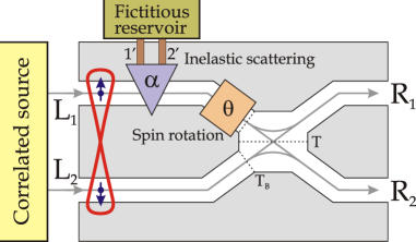
Figure 1: (Color online) The beam splitter geometry fed with pairwise non-locally entangled electron currents or polarized currents. The action of the spin rotation via Rashba spin-orbit coupling in one of the input leads changes noise in the output leads dramatically. Inelastic transport is modeled between the entangler and the spin rotation region by means of one or more fictitious probes. Shot noise measured in terminal $R_{1}$ as a function of $\theta$ can be used to detect the nature of the incoming electron correlations.

The system we will study is depicted in Fig. 1. It is an electronic beam splitter patterned on a two-dimensional electron gas (2DEG) with two (equal length) incoming and two outgoing arms, such that the transmission probability between the upper and the lower arms is $T$. The beam splitter is assumed to have also a finite backscattering amplitude whereby electrons get reflected back into the left leads with probability $1-T_{B}$. We have considered two possibilities for backscattering: the technically simpler case without cross reflection, for which electrons scatter back always into their original incoming leads, and which we will term simple backscattering; and the fully symmetric case, whereby the probability of going from any upper lead to any lower lead remains $T$, be it on the left or the right, which we will call symmetric backscattering. This distinction is only relevant when there is a finite inelastic scattering on the leads, and both give very similar results in any case, so we will focus mainly in the simple backscattering case . Other authors Egues et al. (2005) have previously studied the effect of backscattering in this geometry, although considering that only the electrons in the lead with the backgates can backscatter, whereas in our case the two incoming leads are equivalent (the scattering occurs in the beamsplitter). The effect, as we shall see, is however qualitatively equivalent to their result, which is that backscattering effectively reduces the oscillation amplitude of noise with the spin rotation angle.

We connect the right arms to ground and the two incoming arms to a reservoir that emits non-local spin-correlated electron pairs, biased at a voltage $-V$. For definiteness we choose these pairs so that the $\hat{z}$ spin component of the electron coming at a given time through lead $L_{1}$ is always opposite to that of the corresponding electron coming simultaneously through lead $L_{2}$. They could be or not be entangled, depending on the characteristics of the source and the leads from source to splitter. Time coincidence of pairs is assumed to within a timescale $\tau_{\Delta}$ that is shorter than any other timescale in the system, such as $\Delta t\equiv h/eV$. This implies two constraints. On the one hand, if the source is an entangler such as e.g. that of Refs. Recher et al., 2001; Prada and Sols, 2004, 2005, this would mean that the superconductor emitting the correlated pairs has a large gap $\Delta$ as compared to the bias voltage. On the other hand, the length of the leads connecting the entangler to the beam-splitter device should be of equal length to within $v_{F}\Delta t$ accuracy.

A local spin-rotation in lead $L_{1}$ is implemented by the addition of backgates above and below a section of lead $L_{1}$. Applying a voltage across these backgates the structure inversion asymmetry of the 2DEG is enhanced, inducing a strong Rashba spin-orbit coupling in that region of the 2DEG in a tunable fashion without changing the electron concentration Miller et al. (2003). This in turn gives rise to a precession of the spin around an in-plane axis perpendicular to the electron momentum, which we chose as the $\hat{y}$ axis, resulting in a tunable spin rotation of an angle $\theta$ around $\hat{y}$ after crossing the region with backgates.

The idea behind this setup is that the spin rotation can change the symmetry of the spatial part of the electron pair wavefunction, thus affecting the expected shot noise in the outgoing leads, which is enhanced for even and suppressed for odd spatial wavefunctions. The switching from bunching to antibunching signatures in the shot noise as a function of $\theta$ is enough to identify truly entangled singlets in the incoming current. Likewise, a $\theta$ independent shot noise is an unambiguous signal of a triplet incoming current, since a local rotation of a triplet yields a superposition of triplets, preserving odd spatial symmetry and therefore, antibunching. A current of statistically mixed anticorrelated electron spins can also be distinguished from the entangled cases from the amplitude of the shot noise oscillations with $\theta$. Thus, this device was proposed as a realizable entanglement detector through local shot noise measurements Egues et al. (2002); Burkard and Loss (2003); Egues et al. (2005).

As discussed in the introduction, inelastic scattering due to environmental fluctuations could spoil the physical mechanism underlying this detector, which is Pauli exclusion principle, and should therefore be expected to affect its performance in some way. The implementation of inelastic scattering in ballistic electron systems can be tackled quite simply on a phenomenological level through the addition of fictitious reservoirs within the scattering matrix formalism Blanter and Buttiker (2000). The necessary generalization to deal with entangled currents and a simple scheme to derive the FCS in generic systems with additional fictitious probes is presented in appendix A. We model spin-conserving inelastic scattering by the addition of two fictitious probes (one for spin-up and another for spin-down) in lead $L_{1}$, depicted as a single one in Fig. 1. We have numerically checked that the addition of another two fictitious probes in lead $L_{2}$ gives very similar results for the shot noise through the system, so we will take only two in the upper arm for simplicity. This is also physically reasonable if we consider only decoherence due to the backgates deposited on the upper arm to perform the local Rashba spin-rotation, which provide a large bath of external fluctuations that can cause a much more effective inelastic scattering. The parameter that controls the inelastic scattering probability is $\alpha\in[0,1]$, being $\alpha=1$ the completely incoherent limit.

In the following analysis we will inject into the input arms of the device currents with different types of initial non-local electron-pair density matrix,

$$\hat{\rho}=\frac{1}{2}\left(|L_{1}\!\!\uparrow;L_{2}\!\!\downarrow\rangle\langle L_{1}\!\!\uparrow;L_{2}\!\!\downarrow\!|+|L_{1}\!\!\downarrow;L_{2}\!\!\uparrow\rangle\langle L_{1}\!\!\downarrow;L_{2}\!\!\uparrow\!|\right)$$

$$+\frac{\beta}{2}\left(|L_{1}\!\!\downarrow;L_{2}\!\!\uparrow\rangle\langle L_{1}\!\!\uparrow;L_{2}\!\!\downarrow\!|+|L_{1}\!\!\uparrow;L_{2}\!\!\downarrow\rangle\langle L_{1}\!\!\downarrow;L_{2}\!\!\uparrow\!|\right),$$ (1)

namely, (i) statistical mixtures of up and down classically correlated electrons (diagonal density matrix, $\beta=0$), which we will also call spin-polarized currents, (ii) EPR-type singlet spin-entangled pure states ($\beta=-1$), and (iii) idem with $m_{s}=0$ triplet states ($\beta=1$). We will use subindexes $s$, $t$, and $m$ to denote the pure singlet, pure $m_{s}=0$ triplet and statistically mixed incoming states. Note that this expression refers to pairs of electrons that arrive at the same time at the device, so that this density matrix is actually expressed in a localized wavepacket basis.

Our goal is to ascertain to what extent, for a splitter transmission $T$, a finite backscattering $1-T_{B}$ and finite and unknown amount of inelastic scattering $\alpha$ in the input leads, the shot noise in one of the output arms ($R_{1}$) as a function of rotation angle $\theta$ could still be used to demonstrate the existence or not of initial entanglement, and that way provide a means to distinguish truly quantum-correlated states from statistically correlated (unentangled) ones.

III The technique

In Appendix A we give a detailed account of the method we have used, which can be employed to compute the FCS of a generic mesoscopic conductor with instantaneous current conservation (on the scale of the measuring time) in the attached voltage probes, and generic spin correlations in the incoming currents. We work within the wave packet representation, whereby the basis for electron states is a set of localized in space wavefunctions Martin and Landauer (1992). A sequential scattering approximation is implicit, which however yields the correct $\omega=0$ current fluctuations in known cases with inelastic scattering, see, e.g., Appendix B. We summarize here the main points as a general recipe for practical calculations.

Given a certain mesoscopic system with a number of biased external leads connected to reservoirs, one should add the desired voltage probes to model inelastic scattering (or real probes), and perform the following steps to compute the long-time FCS of the system:

(i) Define the (possibly entangled) incoming states in the external leads for a single scattering event without the probes,

$$|in\rangle=R[\{\hat{a}^{+}\}]|vac\rangle.$$ (2)

Here $R[\{\hat{a}^{+}\}]$ is an arbitrary combination of creation operators $a^{+}_{n}$ of incoming electrons (in the localized wavepacket basis) acting on the system’s vacuum. In our case it would create state (1).

(ii) Add the $N$ two-legged voltage probes (one channel per leg) with individual scattering matrices as in Eq. (11), and compute the total $S$-matrix of the multi-terminal system, $S_{nm}$. Note that $S_{nm}(t,t^{\prime})$ in our temporal basis is assumed to be constant, i.e., independent of $t,t^{\prime}$, which corresponds to an energy independent scattering matrix in an energy basis.

(iii) Define outgoing electron operators $\hat{b}^{+}_{n}=\sum_{m}S_{nm}\hat{a}^{+}_{m}$. To implement instantaneous current conservation we expand our Hilbert space with $N$ integer slave degrees of freedom $\vec{Q}=\{Q_{i}\}$, which result in the following outgoing state after one scattering event,

$$|out;\vec{Q}\rangle\equiv R[\{\hat{b}^{+}\}]\prod_{i}^{N}\left[\hat{b}^{+}_{p_{i};1^{\prime}}\hat{b}^{+}_{p_{i};2^{\prime}}\right]^{g(Q_{i})/2}|vac\rangle.$$ (3)

These $Q_{i}$ are counters of total charge accumulated in the probes. The notation here is that $\hat{b}^{+}_{p_{i};l}$ creates the scattered state resulting from an electron injected through leg $l=\{1^{\prime},2^{\prime}\}$ of the two-legged probe $i$. $g(Q)$ encodes the response of the probe to a certain accumulated charge $Q$. The specific form of $g(Q)$ is not essential as long as it tends to compensate for any charge imbalance in the probe. One convenient choice is given in Eq. (25), which yields in our setup a minimal tripled-valued fluctuation interval of $Q_{i}\in[-1,1]$. Note also that state $|out;\vec{Q}\rangle$ in the above equation is nothing but $U_{\Delta t}|\phi^{e}_{j}\vec{Q}\rangle$ of Appendix A.

(iv) Compute the $3^{N}\times 3^{N}$ $\overline{W}$ matrix

$$\overline{W}_{\vec{Q}_{b}\vec{Q}_{a}}(\vec{\lambda})=\langle out;\vec{Q}_{a}|\hat{P}_{\vec{Q}_{b}}\hat{\chi}_{j}(\vec{\lambda})|out;\vec{Q}_{a}\rangle,$$ (4)

which we write in terms of the moment generating operator $\hat{\chi}_{j}=e^{i\sum_{n}\lambda_{n}(\hat{N}^{\mathrm{out}}_{n}-\hat{N}^{\mathrm{in}}_{n})}$, where $\hat{N}$ are the number operators of electrons scattering in event $j$. The operator $\hat{P}_{\vec{Q}_{b}}$ projects onto the subspace of electron states that have a total of ${Q_{b}}_{i}-g({Q_{a}}_{i})$ particles scattered into probe $i$, i.e., states in which the probe $i$ has gone from ${Q_{a}}_{i}$ to ${Q_{b}}_{i}$ excess electrons. If the incoming state is not a pure state, one should perform the statistical averaging over the relevant $|out;\vec{Q}\rangle$ states at this point.

(v) Compute the resulting long-time current moment generating function $\chi_{I}(\vec{\lambda})$ by taking the maximum eigenvalue of matrix $\overline{W}$. The charge generating function $\chi(\vec{\lambda})$ is obtained simply by taking the power $M$ of $\chi_{I}(\vec{\lambda})$, cf. Eq. (27), where $M=eVt/h$ is the average number of emitted pairs from the source after an experiment time $t$ at a bias $V$.

We make use of this method in our particular system by setting a single counting field $\lambda$ on output lead $R1$, where we wish to compute current fluctuations. This way we derive results for $\chi_{I}$ and current cumulants [see Eqs. (28) and (29)] from the corresponding $\overline{W}$ matrix (4) for the different types of injected currents of Eq. (1).

While explicit expressions for the current cumulant generating function $\ln\chi_{I}(\lambda)$ are in general impossible due to the large dimensions of the $\overline{W}$ matrix ($9\times 9$ in this case), it is always possible to write $\chi_{I}$ in an implicit form that is just as useful to sequentially compute all cumulants, namely, the eigenvalue equation

$$\det\left[\overline{W}(\lambda)-\chi_{I}(\lambda)\bm{1}\right]=0,$$ (5)

supplemented by the condition $\chi_{I}(0)=1$. By differentiating this equation around $\lambda=0$ a number of times and using (28), one can obtain the various zero-frequency current cumulants on arm $R1$.

In the next section, instead of giving the general expression of $\overline{W}$, which is rather large, we provide the explicit expressions for $\chi_{I}$ and shot noise obtained in various useful limiting cases, together with plots of the first cumulants in the $\{T,T_{B},\alpha,\theta\}$ parameter space.

IV Results

In this section we will analyze the performance of the beam splitter device of Fig. 1 as a detector of quantum correlations in the incoming currents through the shot noise or higher current cumulants induced in arm $R_{1}$. We will first make connection with the results in the literature Egues et al. (2002) by computing the shot noise in an elastic splitter, and then we will generalize them to finite inelastic scattering probabilities and finite backscattering. We will thus establish tolerance bounds for such imperfections in the detector. Finally, we will address the question of whether the measurement of higher order current cumulants could improve the tolerance bounds of the device.

IV.1 Shot noise

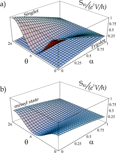
Figure 2: (Color online) In the upper plot (a) we represent the current shot-noise in units of $e^{3}V/h$ in lead $R1$ for the singlet and $m_{s}=0$ triplet incoming states, as a function of spin rotation angle $\theta$ and decoherence strength $\alpha$. The same for the polarized spin state case is presented in the lower plot (b). Inter-lead transmission probability between upper and lower arms $T$ is fixed to $0.5$, and no backscattering ($T_{B}=1$) is assumed.

In the elastic transport limit $\alpha=0$ and with arbitrary intralead backscattering strength $1-T_{B}$, the following expression for the shot noise is obtained,

$$S=\frac{e^{3}|V|}{h}T_{B}\left[1-T_{B}+(1-\beta)T_{B}T(1-T)(1+\cos\theta)\right],$$ (6)

where constant $\beta$ corresponds to the different types of incoming current, cf. Eq. (1). Note that this expression holds for simple or symmetric backscattering (as defined in Sec. II). As shown by Eq. (6), for $\alpha=0$ the amplitude of the $\theta$ dependence is enough to distinguish between the different types of states, if $T$ and $T_{B}$ are known. As could have been expected, the triplet current noise ($\beta=1$) is $\theta$ independent, since the local spin rotation only transforms the $m_{s}=0$ triplet to a different superposition of the other triplet states, none of which can contribute to noise since each electron can only scatter into different outgoing leads due to the Pauli exclusion principle.

However, in the presence of a strong coupling to the environment, $\alpha=1$, the shot noise behaves very differently. Due to the complete incoherence of scattering, which changes the orbital quantum numbers (or arrival times at the detector) of the incoming states, the bunching-antibunching switching disappears. Therefore $S_{s}$, $S_{t}$ and $S_{m}$ become equal and $\theta$ independent. In particular, for simple backscattering we have

$$S_{s}= S_{t} =S_{m}=\frac{e^{3}|V|}{h}\frac{T_{B}}{(1+T_{B})^{3}}\left[1+2T_{B}^{2}T(1-T)\right.$$ (7)

$$\left.-T_{B}(1+3T^{2}-6T)-T_{B}^{3}T^{2}(2+T_{B})\right].$$

These features are illustrated in Fig. 2, where we have plotted the current shot-noise in lead $R_{1}$, normalized to the constant $e^{3}V/h$, as a function of the spin rotation angle $\theta$ and the decoherence parameter $\alpha$, at $T_{B}=1$ and $T=1/2$:

$$\frac{S_{s}}{e^{3}V/h} = \frac{1}{2}\left[1-(\alpha-1)\cos\theta\right]-\frac{\alpha}{32}(5+3\alpha),$$ (8)

$$\frac{S_{t}}{e^{3}V/h} = \frac{\alpha}{32}(11-3\alpha),$$ (9)

$$\frac{S_{m}}{e^{3}V/h} = \frac{1}{4}\left[1-(\alpha-1)\cos\theta\right]-\frac{\alpha}{32}(3-3\alpha).$$ (10)

Note that at $\theta=\pi$ these three shot noise curves are all equal. Note furthermore that for $\alpha=1$ we have $S_{s}=S_{t}=S_{m}=(e^{3}V/h)T(1-T)$ which is $1/4$ in normalized units. The cosine-type dependence of the current noise with $\theta$, $S(\theta)=S(\pi)+\Delta S\cos^{2}(\theta/2)$, where $\Delta S=S(\theta=0)-S(\theta=\pi)$, holds for any value of $\alpha<1$ in the singlet and polarized cases. The oscillation amplitude of the noise for the singlet case is always twice the oscillation amplitude of the polarized one. In contrast, the triplet shot noise (and all higher cumulants for that matter) remains always $\theta$ independent for any $\alpha$ and $T_{B}$.

Since our aim in this study is to find a way to distinguish between the different incoming states of Eq. (1), we will disregard from now on the trivial case of the triplet current, which is easily detectable by its $\theta$-independence, and focus entirely on the distinction between the singlet and mixed state cases. In these two cases, when $T_{B}<1$, the oscillatory behavior with $\theta$ remains, although it is no longer purely sinusoidal. Besides, its oscillation amplitude quickly decreases with increasing backscattering, making the entanglement detection scheme harder. However, we will now show that, knowing only the value of the shot-noise at zero spin rotation angle (or alternatively the amplitude $\Delta S$), it is possible to distinguish between the different incoming states for not-too-strong decoherence.

IV.2 Robust entanglement detection scheme

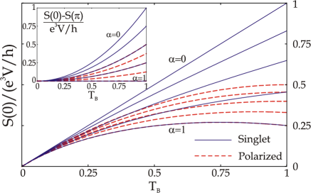
Figure 3: (Color online) Normalized value of shot-noise in lead $R_{1}$ at zero spin rotation angle as a function of beam splitter transmission $T_{B}$ for $T=0.5$. Solid (blue) lines correspond to singlet incoming current whereas dashed (red) lines account for the polarized one. In both cases, different values of inelastic scattering probability have been considered, from $\alpha=0$ (upper curves) to $\alpha=1$ (lower curves) in steps of $0.25$. Inset: the same for the oscillation amplitude with $\theta$ of the shot-noise.

Tuning once again the beam splitter to the symmetric $T=1/2$ point, which turns out to be the optimum point of operation for entanglement detection, we notice from Fig. 2 that the analysis of the $\theta$ dependence of the shot-noise at an arbitrary and unknown value of $\alpha$ indeed precludes from a clear distinction of the singlet and mixed state cases.

A more complete picture can be obtained by plotting the value of the shot-noise at $\theta=0$ in the interval $\alpha\in[0,1]$ as a function of $T_{B}$. This is done in Fig. 3 for the case of simple backscattering. Solid (blue) lines correspond to singlet incoming current, and dashed (red) lines to the polarized one. Moreover, the upper curve in both sets of curves accounts for the case of $\alpha=0$, and for the next ones the value of the inelastic scattering parameter increases, in steps of $0.25$, until $\alpha=1$ for the lower curves (which coincide for both the entangled and polarized cases). The same analysis can be done for the behavior of the amplitude $\Delta S$ as a function of $T_{B}$, as shown in the inset of Fig. 3 (given also for simple backscattering). In this latter case, the amplitudes for both the singlet and the polarized currents have in fact a very simple analytical form, the singlet case ranging from $T_{B}^{2}$ to $0$ and the polarized one from $T_{B}^{2}/2$ to $0$ as we sweep from $\alpha=0$ to $\alpha=1$. Therefore, we see how the $\theta$-independent background noise introduced by the finite backscattering in the main plot of Fig. 3, which could in principle degrade the performance of the entanglement detector as mentioned in Ref. Burkard and Loss, 2003, can be filtered out by measuring the amplitude $\Delta S$. We also note that if a symmetric backscattering is considered, the resulting curves for Fig. 3 are qualitatively the same, and therefore it does not affect the above discussion.

We can observe in both plots of Fig. 3 that if $\alpha$ is unknown, as it is usually the case in an experiment, the classical and quantum currents are distinguishable from a single noise measurement (or two in the case of the inset) only if its value is found to lie outside of the overlapping region between the two sets of curves. According to this model, this should always happen for values of inelastic scattering smaller than at least one half. In the case of the main figure, even higher values of $\alpha$ can be distinguished for values of $T_{B}$ close to one. In any case, the values of $\alpha$ for which the noise measurement is no longer able to distinguish a singlet entanglement from a statistically mixed case are rather high, $\alpha\in[0.5,1]$. This means that, in a realistic situation where decoherence is not too strong, shot-noise measurements remain enough for determining if the source feeding the beam-splitter is emitting entangled or statistically mixed states.

IV.3 Higher order cumulants

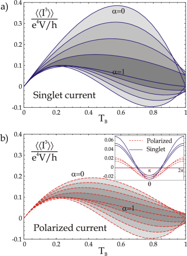
Figure 4: (Color online) Oscillation range with angle $\theta$ of the skewness in lead $R_{1}$, in units of $e^{4}V/h$, as a function of beam-splitter transmission between left and right arms $T_{B}$. $T$ is fixed to the optimal point $T=0.5$. Different oscillation ranges for different values of inelastic scattering are indicated by different shades of gray, ranging from pale gray for $\alpha=0$ to dark gray for $\alpha=1$ in steps of 0.25. The case of singlet-entangled incoming current is considered in plot (a), whereas in plot (b) the incoming current is in a polarized state. The actual oscillation of skewness with Rashba spin rotation angle for entangled current (solid blue lines) and polarized current (dash red lines) is plotted in the inset of (b) (see main text).

We could ask whether it is possible to distinguish between incoming singlet-entangled and polarized currents for a wider range of parameters $\alpha$ by analyzing higher order cumulants. The short answer is ”no”.

As we did for the noise in Fig. 2, we can plot the angular dependence of the third moment, the skewness, for different values of inelastic scattering parameter $\alpha$. This is shown in a 2D plot in the inset of Fig. 4(b) for $T=0.5$ and $T_{B}=1$. As before, solid (blue) lines and dashed (red) lines correspond to spin singlet-entangled and polarized incoming currents, respectively. Now we find that the behavior of skewness with $\theta$ is not monotonous as $\alpha$ varies. For $\alpha=0$ and $\alpha=1$ at $T_{B}=1$ the third cumulant is zero for every angle both for entangled and for mixed states (the probability distribution of the current is symmetric for those parameters as was previously noted in the $\alpha=0$ case in Ref. Taddei and Fazio (2002)). Moreover, this means that the skewness is not a good entanglement detector for a near perfect beam splitter, nor when the inelastic scattering is strong. For intermediate values of decoherence, still at $T_{B}=1$, the skewness oscillates with the spin rotation angle and its oscillation amplitude, $\langle\langle I^{3}\rangle\rangle(\theta=0)-\langle\langle I^{3}\rangle\rangle(\theta=\pi)$, has a maximum around $\alpha\approx 0.5$. This oscillation range is depicted in the main plots of Fig. 4 as a function of the transmission between left and right arms $T_{B}$ (where simple backscattering has been considered). Several values of the inelastic parameter are differentiated using different shades of gray, ranging from pale gray for $\alpha=0$ to dark gray for $\alpha=1$ in steps of 0.25. The main features can be summarized as follows. First, both for the entangled and the polarized current, the broadest oscillation range occurs for $\alpha=0$ (being bigger for the singlet-entangled case). Second, for $\alpha=1$ the oscillation amplitude in both cases is zero, although the skewness remains finite and positive (shifting from a Gaussian to a Poissonian distribution of current as $T_{B}$ goes from $1$ to $0$). For $T_{B}$ smaller than $0.9$ approximately, the behavior of the oscillation range is monotonous with $\alpha$, it simply decreases with it. For small values of $T_{B}$, the skewness coincides with the shot-noise, which is expected since the probability distribution for a tunnel barrier recovers a Poisson distribution, even in the presence of inelastic scattering. In general, the sign of the skewness is reversed in a wide range of parameters by tuning the spin rotation $\theta$.

Concerning our entanglement detection motivation, comparing Fig. 4(a) and 4(b) we find that the third cumulant does not provide any further information in our search of a way to distinguish between entangled and non-entangled incoming states. For $T_{B}$ of the order of $0.9$ and above, due to the non-monotonous behavior of the oscillation range with $\alpha$, the skewness of our beam splitter setup can hardly be used as a detector of entanglement at all. For smaller values of $T_{B}$, we are able to discriminate between different currents in the same range of inelastic scattering parameter $\alpha$ as we could with the noise, this is, from zero decoherence to roughly $\alpha=0.5$.

We have also analyzed further cumulants, whose behaviors with $T_{B}$ and $\theta$ get more intricate as the order of the cumulant increases, and have found the same qualitative result. Either they are not useful tools for entanglement detection or the range of parameters $\alpha$ and $T_{B}$ is not improved from what we find with the shot-noise measurements.

V Conclusions

In this work we have analyzed the effect of inelastic scattering, modeled by spin-current conserving voltage probes, on entanglement detection through a beam-splitter geometry. We have shown that the action of inelastic processes in the beam-splitter cannot be neglected, since it directly affects the underlying physical mechanism of the detector, which is the fact that two electrons with equal quantum numbers cannot be scattered into the same quantum channel. If there is a finite inelastic scattering, such antibunching mechanism is no longer perfect, and the entanglement detection scheme has to be revised.

However, we have found that detection of entanglement through shot noise measurements remains possible even under very relaxed conditions for imperfections in the beam-splitter device and substantial inelastic scattering. Even if a reliable microscopic description of inelastic processes is not available, the present analysis suggests that the detection scheme is robust for inelastic scattering probabilities up to $50\%$.

We have also shown that higher current cumulants do not contain more information about the entanglement of the incoming currents than the shot noise. We have analyzed in particular the skewness of current fluctuations, finding that finite backscattering and inelastic scattering strongly affect the asymmetry of current fluctuations. In particular, a positive skewness is developed as the beam splitter transparency is lowered.

Finally, we have developed a novel way to implement current conservation in voltage probe setups when the incoming currents are non-locally spin correlated, which can be applied to a wide variety of problems where entanglement is key.

Appendix A Phenomenological description of inelastic scattering

Voltage probes are frequently real components of mesoscopic devices, but have also been used traditionally for phenomenological modeling purposes. The voltage probe description of inelastic scattering resorts to the addition of one or more fictitious reservoirs and leads attached to the coherent conductor under study through specific scattering matrices, around the regions where inelastic scattering is to be modeled. While being still coherent overall, the elimination of the fictitious reservoirs results in an effective description of transport such that electrons that originally scattered into the reservoirs now appear as having lost phase and energy memory completely.

We will now discuss the implementation of the voltage probe in the presence of charge relaxation and general incoming states. The whole idea of the voltage probe is to use the non-interacting scattering formalism to model inelastic electron scattering, and the crossover from coherent conductors to incoherent ones. There are two ways to do this. The simpler one assumes a static chemical potential in the probes that is computed self-consistently by fixing time-averaged current flowing into the probes to zero, as corresponds to an infinite impedance voltage probe, or to inelastic scattering. This gives a physically sound conductance value, but fails to yield reasonable shot noise predictions. The reason is that total current throughout the system should be instantaneously conserved. The more elaborate way, therefore, assumes fluctuations in the state of the probe that can compensate the current flowing into the probe(s) at any instant of time (and possibly also energy if one is modeling pure elastic dephasing deJong and Beenakker (1996); vanLangen and Buttiker (1997); Chung et al. (2005)), which gives results for current fluctuations in agreement with classical arguments Blanter and Buttiker (2000).

It is traditional to impose such constraint within a Langevin description of current fluctuations Beenakker and Buttiker (1992), whereby the chemical potential in the probe is allowed to fluctuate, but the intrinsic formulation of this approach makes it inadequate to treat the statistics of general incoming (entangled or mixed) states, other than those produced by controlling individual chemical potentials. There seems to be no known way of how to include the effect of arbitrary correlations between electrons, such as e.g. non-local quantum spin correlations, which are precisely the contributions we are interested in this work. The technique we will develop in the following explicitly takes into account the precise incoming state of the electrons, and recovers results obtained within the Langevin approach in the case of non-correlated incoming states. For an analysis of the possibility of implementing these correlation effects within the Langevin approach and for a comparison to the present (time-resolved) technique, see Appendix B)

The scattering matrix to a (two-legged ) fictitious probe is given, in the basis ${1,2,1^{\prime},2^{\prime}}$ (being $1^{\prime},2^{\prime}$ the extra leads), by

$$S_{\alpha}=\left(\begin{array}[]{cccc}0&-\sqrt{1-\alpha}&i\sqrt{\alpha}&0\\ \sqrt{1-\alpha}&0&0&i\sqrt{\alpha}\\ i\sqrt{\alpha}&0&0&\sqrt{1-\alpha}\\ 0&i\sqrt{\alpha}&-\sqrt{1-\alpha}&0\end{array}\right),$$ (11)

with $\alpha$ being the inelastic scattering probability. This should be composed together with any other scattering matrices in the system, and any other probes present. In a spinful case in which inelastic scattering does not flip spin there should be at least two of these probes, one per spin channel. Other considerations such as inelastic channel mixing in multichannel cases should be taken into account when designing the relevant fictitious probe setup. Let us first consider a general setup with a single probe for simplicity.

We will now introduce the implementation of charge conservation through the system (i.e. in the fictitious probe) which will lead to the simple result expressed in Eq. (26). We first make the essential approximation that the inelastic scattering time in the interacting region is much smaller than

$$\Delta t\equiv h/eV.$$ (12)

The inverse of the timescale $\Delta t$ is the average rate at which the external leads inject particles into the system, in the localized wave-packet terminology Martin and Landauer (1992). We will call the scattering processes within time interval $\Delta t$ a ‘scattering event’. In this limit of quick scattering we can assume sequential scattering events, as if each $\Delta t$ interval was an independent few-particle scattering problem, one for each time

$$t_{j}\equiv j\Delta t.$$ (13)

The overlap of the wave-packets which would in principle give contributions away from the sequential scattering approximation is assumed to have a negligible effect in the long time limit. Other works in different contexts Shelankov and Rammer (2003) seem to support this statement. Furthermore, if one considers small transparency contacts between the electron source and the fictitious probes, the sequential scattering approximation is also exact.

The incoming state in each scattering event will be one particle in each channel of the external leads ($L_{1}$ and $L_{2}$ in the setup of Fig. 1), plus a certain state in the probe’s leads $1^{\prime}$ and $2^{\prime}$. This state injected from the probe is prepared in a way so as to compensate for excess charge scattered into the fictitious probe in all previous events, with the intention of canceling any current that has flowed into the probe in the past. The book-keeping of the probe’s excess charge is done via an auxiliary slave degree of freedom $|Q\rangle$ with discrete quantum numbers $Q=0,\pm 1,\pm 2,\dots$ that count charge transferred to the probe. The incoming state in leads $1^{\prime}$ and $2^{\prime}$ injected by the probe into the system is a function of $Q$. The time evolution of the slave state $|Q\rangle$ is constrained so that $Q$ always equals the total number of electrons that has entered the probe since the first scattering event. In particular, the time evolution of $|Q\rangle$ during one scattering event $\Delta t$ is taken to follow the resulting net charge that was transferred to the probe during that event. This scheme effectively correlates the initially uncorrelated scattering events in order to satisfy instantaneous current conservation through the system, where by instantaneous we mean at times larger than $\Delta t$ but still much smaller than the measuring time.

If the incoming state in the probe’s leads is chosen correctly, the number of $Q$ states between which $|Q\rangle$ will fluctuate during many scattering events will be bounded, and will be independent of the total number of events

$$M=eVt/h$$ (14)

in the total experiment time $t$. This is the underlying principle of this approach, which will guarantee that the instantaneous charge fluctuations in the probe will be bounded to a few electrons throughout the whole measurement process, i.e., the probe current will be zero and noiseless at frequencies below $eV/\hbar$.

The choice that minimizes the charge fluctuations in a single channel two-legged probe in the absence of superconductors in the system is the following: if $Q$ at the beginning of the scattering event is $1$ or $2$, the probe will emit two particles, one through each ’leg’, thereby losing a maximum of $2$ and a minimum of $0$ in that event; if $Q$ is $0$, $-1$ or $-2$ the probe will not emit any particle, thereby absorbing a maximum of $2$ and a minimum of $0$. The resulting fluctuations of $Q$ are bounded in the $[-2,2]$ range. In some cases, such as the system discussed in the main text, this range is reduced to $[-1,1]$ since the entangler only emits one electron of each spin in each scattering event, so that the probe will never absorb $2$ particles, but a maximum of $1$. The relevance of this discussion will be apparent in connection with Eq. (21), since it will determine the dimensions of the $W$ operator therein.

A.1 Sequential scattering scheme for the Full Counting Statistics

We wish to compute in a general case the characteristic function

$$\chi(\vec{\lambda};M)=\langle e^{i\sum_{n}\lambda_{n}\Delta\hat{N}_{n}}\rangle=\mathrm{Tr}\left\{\hat{\chi}(\vec{\lambda})\rho(t)\right\}$$ (15)

after a total measuring time interval $t$. Number difference $\Delta\hat{N}_{n}\equiv\hat{N}^{\mathrm{out}}_{n}-\hat{N}^{\mathrm{in}}_{n}$ is defined as the number operator in channel $n$ at time $t$ (scattered outgoing particle number) minus the number operator at time zero, before any scattering (incoming particle number). Differentiating $\ln\chi$ respect to the counting fields $\lambda_{n}$ one obtains the different transferred charge and current cumulants, Eq. (28).

Let us include the fictitious probe and expand our Fock space with the slave degree of freedom $|Q\rangle$. We take the density matrix of the whole system at time zero equal to $\rho(0)=\rho^{Q}(0)\otimes\rho^{e}(0)$, the second $\rho$ being the electronic density matrix. As we will see we do not need to specify the initial state of the slave degree of freedom $\rho^{Q}(0)$ since it will not affect our results in the long time limit. The density matrix is factorized in the localized wave-packet basis Martin and Landauer (1992),

$$\rho(0)=\rho^{Q}(0)\otimes\prod_{j}^{\otimes}\rho^{e}_{j},$$ (16)

with the electronic part being $\rho^{e}_{j}\equiv\rho^{r}_{j}\otimes\rho^{p}_{j}$. Each of these $\rho^{e}_{j}$ constitutes the incoming state in each of the $j$ scattering events corresponding to the time interval $[t_{j},t_{j+1}]$. $\rho^{r}_{j}$, which is actually $j$-independent, is the density matrix of the (uncorrelated in time) electrons coming from the external reservoirs, and $\rho^{p}_{j}$ is the density matrix of the (correlated in time-through-$Q$) electrons coming from the fictitious probe. As we mentioned, this matrix $\rho^{p}_{j}$ will depend on the state of the slave degree of freedom $Q$ at the beginning of each scattering event $j$.

The time evolution from 0 to $t$, $\rho(t)=\hat{U}_{t}\rho(0)\hat{U}^{+}_{t}$ is split up in the $M$ time intervals of length $\Delta t$. The sequential scattering approximation amounts to assuming that in each event each electron group $\rho^{e}_{j}$ scatters completely before the next one does. Therefore $\hat{U}_{t}=\hat{U}_{\Delta t}^{M}$. We defer the discussion on how $U_{\Delta t}$ operates precisely to a little later.

Since operator $\hat{\chi}(\vec{\lambda})$ will factorize into contributions for each scattering event, $\hat{\chi}=\prod_{j}\hat{\chi}_{j}$, we can rewrite equation (15) as

$$\chi = \mathrm{Tr}_{Q}\left\{\mathrm{Tr}_{M}\left[\hat{\chi}_{M}U_{\Delta t}\rho^{e}_{M}\mathrm{Tr}_{M-1}\left[\right.\right.\right.\cdots$$

$$\cdots \left.\left.\left.\mathrm{Tr}_{1}\left[\hat{\chi}_{1}U_{\Delta t}\rho^{e}_{1}\rho^{Q}(0)U^{+}_{\Delta t}\right]U^{+}_{\Delta t}\right]U^{+}_{\Delta t}\cdots\right]\right\},$$

where $\mathrm{Tr}_{j}$ stands for the trace over the $\rho^{e}_{j}$ electron states and $\mathrm{Tr}_{Q}$ over the $Q$ subspace. An alternative way of writing this is by induction. Defining an auxiliary operator $\hat{\Phi}^{(k)}=\sum_{QQ^{\prime}}|Q\rangle\Phi^{(k)}_{QQ^{\prime}}\langle Q^{\prime}|$ such that

$$\hat{\Phi}^{(j)} = \mathrm{Tr}_{j}\left[\hat{\chi}_{j}U_{\Delta t}\rho^{e}_{j}\hat{\Phi}^{(j-1)}U^{+}_{\Delta t}\right],$$ (18)

$$\hat{\Phi}^{(0)} = \rho^{Q}(0),$$ (19)

one can see that (A.1) and (15) are equivalent to

$$\chi(\vec{\lambda};M) = \mathrm{Tr}_{Q}\hat{\Phi}^{(M)}.$$ (20)

After some algebra, Eq. (18) can be recast into the following sum over the total range of $Q$ values,

$$\Phi^{(j)}_{Q_{b}Q_{b}^{\prime}}=\sum_{Q_{a}Q_{a}^{\prime}}W^{Q_{a}Q_{a}^{\prime}}_{Q_{b}Q_{b}^{\prime}}\Phi^{(j-1)}_{Q_{a}Q_{a}^{\prime}},$$ (21)

with the $W$ superoperator

$$W^{Q_{a}Q_{a}^{\prime}}_{Q_{b}Q_{b}^{\prime}}(\vec{\lambda})=\mathrm{Tr}_{j}\left[P_{Q_{b}^{\prime}Q_{b}}\hat{\chi}_{j}(\vec{\lambda})U_{\Delta t}\rho^{e}_{j}P_{Q_{a}Q_{a}^{\prime}}U^{+}_{\Delta t}\right],$$ (22)

and $P_{QQ^{\prime}}\equiv|Q\rangle\langle Q^{\prime}|$ the generalized projector within the slave degree of freedom space. We will specify how it operates in practice a bit later, after Eq. (24).

Some words about the meaning of this operator $W$, which is a central object in this technique, are in order at this point. It is a superoperator that, for $\vec{\lambda}=0$ simply transforms the reduced density matrix $\rho^{Q}(t_{j})=\hat{\Phi}^{(j)}(\vec{\lambda}=0)$ of the slave degree of freedom at time $t_{j}$ to the subsequent one $\hat{\Phi}^{(j+1)}(\vec{\lambda}=0)$ at time $t_{j+1}$. In Eq. (18) we see how $\hat{\Phi}^{(j)}$ is simply $\hat{\Phi}^{(j-1)}$ to which the incoming state $\rho^{e}_{j}$ for event $j$ is added, is allowed to evolve a time $\Delta t$ (during which also $\rho^{Q}$ evolves as dictated by the number of electrons scattered into the probe), and the scattered electrons are traced out. The result is the new evolved reduced density matrix for the slave degree of freedom. For finite $\vec{\lambda}$, the corresponding counting fields for the scattered electrons are also included into $\hat{\Phi}^{(j)}$ so as to be able to recover the desired cumulants of the traced-out electrons after time $t$ from $\chi=\mathrm{Tr}_{Q}\hat{\Phi}^{(M)}$. This can be also seen as supplementing the dynamics of the system with a quantum field term $\propto\lambda_{n}$ in the action, in the generalized Keldysh language of Ref. Nazarov, 1999.

By assuming without loss of generality a diagonal initial $\rho^{Q}(0)$ and by noting that, by construction, states with different $Q$ are orthogonal, we can in general take $W$ to be diagonal $W^{Q_{a}Q_{a}^{\prime}}_{Q_{b}Q_{b}^{\prime}}=\delta_{Q_{a}Q_{a}^{\prime}}\delta_{Q_{b}Q_{b}^{\prime}}\overline{W}_{Q_{b}Q_{a}}$, and $\Phi^{(j)}_{QQ^{\prime}}=\delta_{QQ^{\prime}}\Phi^{(j)}_{Q}$. Physically this means that sequentially taking out of the system the scattered electrons (tracing them out) forbids the $Q$ counter to remain in a coherent superposition, since the electron that generated it has been ‘measured’. Therefore (20) finally becomes

$$\chi(\vec{\lambda};M)=\sum_{Q_{a}Q_{b}}\overline{W}^{M}_{Q_{b}Q_{a}}\rho^{Q}_{Q_{a}Q_{a}}(0)$$ (23)

(note the $M^{\mathrm{th}}$ power of the $\overline{W}$ matrix). The following alternative and useful form for (22) can be obtained by writing $|Q\rangle\langle Q|\rho^{e}_{j}|Q\rangle\langle Q|=|\phi^{e}Q\rangle\langle\phi^{e}Q|$, in the case of a pure incoming state in the external leads,

$$\overline{W}_{Q_{b}Q_{a}}(\vec{\lambda})=\langle\phi^{e}Q_{a}|U^{+}_{\Delta t}P_{Q_{b}Q_{b}}\hat{\chi}_{j}(\vec{\lambda})U_{\Delta t}|\phi^{e}Q_{a}\rangle,$$ (24)

where $|\phi^{e}Q\rangle$ stands now for the incoming electronic state (through all leads) that corresponds to a given value $Q$ of the slave degree of freedom.

Let us analyze the action of the evolution operator $U_{\Delta t}$ in the above equation. Since we assume that particles scatter fully in time $\Delta t$, the action of $U_{\Delta t}$ on the electrons is written in terms of the global scattering matrix $b^{+}_{n}=U_{\Delta t}a^{+}_{n}U^{+}_{\Delta t}=\sum_{m}S_{nm}a^{+}_{m}$, where $a^{+}_{n}$ are the electron creation operators in the different leads (including fictitious ones) of the system . The effect of $U_{\Delta t}$ on the $\hat{Q}$ degree of freedom is merely to update it with the net number of electrons scattered into the fictitious leads, fixing $\hat{Q}_{t_{j+1}}-\hat{Q}_{t_{j}}=\Delta\hat{N}_{p}$, where $\Delta\hat{N}_{p}$ is the number of electrons absorbed by the probe in the event. This implies that $P_{Q_{b}Q_{b}}$ in Eq. (24), which projects on the subspace with $Q=Q_{b}$, can be substituted by the electron-only operator that projects over scattered electronic states that satisfy $\hat{N}^{\mathrm{out}}_{p}=\hat{N}^{\mathrm{in}}_{p}+Q_{b}-Q_{a}$, where $\hat{N}^{\mathrm{out}}_{p}$ is the number operator for fermions scattered into the probe, $\hat{N}^{\mathrm{in}}_{p}$ is the number of electrons incident from the probe into the system at the beginning of the scattering event, and $Q_{a}$ is the value of $Q$ also at the beginning of the scattering event.

As anticipated just before the beginning of this subsection, the value of $\hat{N}^{\mathrm{in}}_{p}$ on $|\phi^{e}Q_{a}\rangle$ is a function of $Q_{b}$, and should be chosen properly so as to compensate for a given excess probe charge $Q_{a}$ at the beginning of a given scattering event. That way the fluctuations of the probe’s excess charge $Q$ will be minimum, although the precise choice does not affect the result as long as the resulting range of fluctuations of $Q$ does not scale with measurement time $t$. As already discussed, for most cases the optimum choice is $N^{in}_{p}(Q)=g(Q)$, with

$$g(1) = 2~{}~{}~{}\textrm{(one electron in each lead of the probe)},$$

$$g(0) = g(-1)=0,$$ (25)

which gives $Q\in[-1,1]$, and a $3\times 3$ $\overline{W}$ matrix.

To finish with the discussion of Eq. (24), recall that $\hat{\chi_{j}}=e^{i\sum_{n}\lambda_{n}(\hat{N}^{\mathrm{out}}_{n}-\hat{N}^{\mathrm{in}}_{n})}$ and that a useful relation for the case of a single channel mode $n$ in which the eigenvalues of $\hat{N}_{n}$ are zero and one is $e^{i\lambda_{n}\hat{N}_{n}}=1+(e^{i\lambda_{n}}-1)\hat{N}_{n}$.

The whole Levitov-Lee-Lesovik formulation of FCS Levitov et al. (1996) is well defined only in the long time limit. In such limit it is clear that expression (24) is dominated by the biggest eigenvalues $\mu_{\mathrm{max}}$ of $\overline{W}$. All of its eigenvalues satisfy $|\mu|\leq 1$ for real values of $\vec{\lambda}$, so that those that are not close to 1 for small values of $\vec{\lambda}$ (around which we take derivatives to compute cumulants) will exponentiate to zero when $M\rightarrow\infty$. In all cases we examined only one eigenvalue $\mu_{\mathrm{max}}$ would not exponentiate to zero, although it can have finite degeneracy. In general, we have the following asymptotic property, valid for any degeneracy of $\mu_{\mathrm{max}}$,

$$\ln\left[\chi(\vec{\lambda};M)\right]=M\ln\left[\mu_{\mathrm{max}}\right]+\mathcal{O}(1).$$ (26)

We can define a new generating function

$$\ln\chi_{I}(\vec{\lambda})=\lim_{M\rightarrow\infty}\frac{\ln\chi(\vec{\lambda};M)}{M}.$$ (27)

It can be shown that this function generates the zero frequency limit of current cumulants

$$\langle\langle I_{n}(\omega=0)^{k}\rangle\rangle=\frac{e^{k+1}|V|}{h}(-i)^{k}\left.\partial^{k}_{\lambda_{n}}\ln\chi_{I}\right|_{\vec{\lambda}=0},$$ (28)

being $e$ here the electron charge and $k$ the order of the cumulant, $k=1$ for the average current, $k=2$ for the shot noise, and so on.

We can identify

$$\chi_{I}(\vec{\lambda})=\mu_{\mathrm{max}}(\vec{\lambda}).$$ (29)

This is our final result. $\mu_{\mathrm{max}}$ is the eigenvalue of Eq. (24) that equals $1$ when all counting fields $\lambda_{n}$ are taken to zero.

The generalization to multiple probes is very straightforward. Given the optimum choice of Eq. (25), the solution of an $N-$probe setup will involve the diagonalization of an $3^{N}\times 3^{N}$ $\overline{W}$ matrix similar to Eq. (24) where $Q$ is changed to $\vec{Q}$, a vector of the $N$ corresponding slave degrees of freedom. On the other hand, to implement charge conservation in probes with more than one channel per leg (or more than two legs), such as non-spin-conserving probes, the formalism would require a slightly different expression for Eq. (25) and a consequently bigger dimension for $\overline{W}$, but would otherwise remain quite the same.

A summary of the above results is given in Sec. III.

We have successfully compared the present method to Langevin techniques in scenarios where the latter is directly applicable (uncorrelated spins), obtaining identical results in all cases. Some simple examples are the FCS of a single channel wire with contact transmissions $T_{1}$ (see Appendix B for the details), the case of a Mach-Zehnder interferometer or an NS junction, for which both this and the Langevin method Beenakker and Buttiker (1992) yield identical results for $\chi_{I}$. We would like to mention that even in the presence of correlated spins the Langevin technique can be extended to include correlation effects to some extent, as is discussed in Appendix B.

Appendix B Comparison of the method to previous techniques

In this appendix we will show with a simple example how the proposed method yields identical results to the ones obtained with previous Langevin technique (applicable in such case), which we generalize here to yield the FCS, instead of individual current cumulants. We also sketch how a Langevin derivation of the beam splitter FCS could be attempted by extending the technique, and a comparison to our results. The purpose of this section is twofold. First we wish to make a convincing case that our method actually recovers known results, but goes beyond them in other cases, and secondly, that it indeed yields the FCS in the presence of an inelastic probe, and not merely a dephasing probe as could be thought from the unusual real time sequential scattering picture.

We will first do our comparison in the possibly simplest system one can think of, a zero-temperature single channel conductor for spinless fermions, see Fig. 5. We will assume symmetric contacts to the (real) reservoirs with transmission $T_{1}$. A fictitious inelastic probe will be connected between the two contacts with transmission amplitude $\alpha$, and scattering matrix (11).

As discussed in detail in Ref. Blanter and Buttiker, 2000, within the Langevin approach, the current fluctuations in the presence of the probe should be corrected by the feedback due to the instantaneous fluctuations of the probes voltage, which react to cancel any current flowing into the probe. Thus the current fluctuation flowing into the right reservoir reads

$$\Delta I_{2}=\delta I_{2}+\frac{T_{2p}}{T_{1p}+T_{2p}}\left(\delta I_{p_{1}}+\delta I_{p_{2}}\right),$$ (30)

where $\delta I_{2}$ correspond to the current fluctuations flowing out of the system through lead $2$ with a static potential in the probe, whereas $\delta I_{p_{1}}$ and $\delta I_{p_{2}}$ are the analogous currents leaving the system through legs $p_{1}$ and $p_{2}$ of the probe. $T_{nm}=T_{mn}$ are the transmission probabilities between channels $m$ and $n$. We make use of the compact notation $T_{np}=T_{n{p_{1}}}+T_{n{p_{1}}}$. The static potential in the probe for $\delta I_{n}$ is chosen so as to cancel any average current into the probe.

In our case, left-right symmetry implies

$$\Delta I_{2}=\delta I_{2}+\frac{1}{2}\left(\delta I_{p_{1}}+\delta I_{p_{2}}\right).$$ (31)

At this point, what one usually finds in the literature is a calculation of cumulants of certain order. It is possible however to compute them all at once and recover the FCS, as we show in the following. Define the characteristic function with a static potential $\mu_{p}=eV/2$ in the probe (the value which gives average current conservation) and with two counting fields, one ($\lambda_{2}$) that counts particles flowing into the rightmost reservoir, and another ($\lambda_{p}$) that counts particles scattered into the probe

$$\chi(\lambda_{2},\lambda_{p})=\langle e^{i\lambda_{2}\Delta N_{2}+i\lambda_{p}(\Delta N_{p_{1}}+\Delta N_{p_{2}})}\rangle.$$ (32)

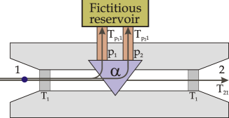
Figure 5: (Color online) Single channel wire geometry with fictitious probe and non-transparent contacts.

Since at this point there are still no probe fluctuations (each energy is independent from the rest), one can write $\chi(\lambda_{2},\lambda_{p})$ as the product of two characteristic functions, one for particles in the interval $[0,\mu_{p}]$ and another in the $[\mu_{p},eV]$Levitov et al. (1996). We have

$$\chi(\lambda_{2},\lambda_{p}) = \langle 1|\hat{\chi}_{2}(\lambda_{2})\hat{\chi}_{p_{1}}(\lambda_{p})\hat{\chi}_{p_{2}}(\lambda_{p})|1\rangle^{M/2}$$ (33)

$$\langle 0|\hat{\chi}_{2}(\lambda_{2})\hat{\chi}_{p_{1}}(\lambda_{p})\hat{\chi}_{p_{2}}(\lambda_{p})|0\rangle^{M/2},$$

where $\hat{\chi}_{n}(\lambda)\equiv 1+\left(e^{i\lambda}-1\right)\hat{N}_{n}$, $|1\rangle$ is the scattered state at an energy below $\mu_{p}$ (i.e., with a full state coming from the probe), and $|0\rangle$ is a state above $\mu_{p}$ (empty probe). Working out the algebra we get for the current characteristic function, Eq. (27),

$$\chi_{I}(\lambda_{2},\lambda_{p}) = \left\{\left[1+(e^{i\lambda_{2}}-1)T_{12}+(e^{i\lambda_{2}-i\lambda_{p}}-1)T_{2p}\right]\right.$$

$$\times\left.\left[1+(e^{i\lambda_{2}}-1)T_{12}+(e^{i\lambda_{p}}-1)T_{2p}\right]\right\}^{\frac{1}{2}},$$

where $T_{12}=T_{1}^{2}(1-\alpha)/[2-\alpha-T_{1}(1-\alpha)]^{2}$ and $T_{2p}=T_{1}\alpha/[2-\alpha-T_{1}(1-\alpha)]$.

To include the self-consistent voltage fluctuations of the probe, we return to Eq. (31). It is easy to see that the function

$$\chi_{I}(\lambda_{2})\equiv\chi_{I}(\lambda_{2},\frac{\lambda_{2}}{2})=1+(e^{i\lambda_{2}}-1)T_{12}+(e^{i\lambda_{2}/2}-1)T_{2p}$$ (34)

generates the cumulants of $\Delta I_{2}$, instead of $\delta I_{2}$, and therefore is the proper FCS solution of the Langevin approach.

On the other hand, the method we have developed involves, in this simple system and for the same choice of $g(Q)$ as in Eq. (25), the following expression of the $\overline{W}$ matrix in (24)

$$\overline{W}=\left(\begin{array}[]{ccc}a&0&0\\ c&a&b\\ 0&c&a\end{array}\right),$$ (38)

with $a=1+(e^{i\lambda_{2}}-1)T_{12}-T_{2p}$, $b=e^{i\lambda_{2}}T_{2p}$ and $c=T_{2p}$. The highest eigenvalue of this matrix is $a+\sqrt{bc}$, which indeed equals the Langevin result (34).

This example clarifies the fact that the fictitious probe we are describing within our approach is inelastic since, as is evident within the Langevin approach, a particle scattered into the probe at a certain energy can abandon it at any other energy in the interval $[0,eV]$. In particular, note that the the current through the system when $T_{1}=1$ and $\alpha=1$ is noiseless, i.e., the Fano factor as derived from Eq. (34) is $F=0$, as opposed to $F=1/4$ that would result from the quasi-elastic probe Blanter and Buttiker (2000).

B.1 Langevin technique with spin correlations

The Langevin language makes use of one crucial assumption, that the currents flowing into the system are those which result from some static chemical potentials in the real non-interacting reservoirs, and which are therefore spin-uncorrelated. Can one use it to compute current fluctuations when the electrons injected into the system are in a tailored spin state, such as non-local spin singlets arriving simultaneously on the beam splitter in the main text (Fig. 1)? The answer is ”no”, but one can actually go quite far in this direction. One can modify the above scheme to try to account for the peculiar spin correlations, although it only works up to the second cumulant, deviations appearing from the third cumulant onward. This works as follows. One could compute the equivalent chemical potential for spin-up and spin-down electrons in each of the incoming leads as if they were completely uncorrelated, but then try to preserve the correlation information by inserting the proper spin-correlated state in Eq. (32). It is rather unclear in this case whether one is thereby assuming that electrons arriving at the same time into the two leads $L_{1}$ and $L_{2}$ are spin entangled, or whether it is electrons with definite and equal energy which are non-locally spin entangled. Remarkably, the result for the shot noise agrees with the one obtained with our time-resolved technique, where these questions are fully under control, but higher cumulants do not. From a mathematical point of view it is hardly surprising that the FCS from both techniques does not agree in the general case, since through Langevin one obtains an explicit form of the generating function in terms of elementary functions, while with the time-resolved technique the latter is the solution of a non-reducible ninth order polynomial, Eq. (5), which is known not to have a closed form in general. The discrepancy between the methods, which is rather small in most cases, is most likely due to the fact that in the Langevin language it is not possible to encode the time-resolved spin correlation information of the incoming current.

Figure 6: (Color online) The results for the singlet current skewness in the beam splitter geometry calculated within the modified Langevin approach begin to deviate slightly from those of the time-resolved (TR) technique, Fig. 4. Note that the deviation is most apparent in the intermediate $\alpha$ limit. Shot noise results are identical. At this level, however, both techniques are qualitatively equivalent.

We now sketch in more detail how the attempt at calculating the FCS of the beam splitter within the Langevin language should go. All chemical potentials are in principle spin-dependent, and transmissions (for $\theta\neq 0$) will connect different spins. The equivalent chemical potential in leads $L_{1}$ and $L_{2}$ is $\mu_{L}^{\sigma}=eV/2$, since only one out of two particles has, say, spin-up. The average chemical potential in the voltage probe reads

$$\mu_{p}^{\sigma}=\frac{eV}{2}\frac{\sum_{\sigma^{\prime}}T_{pL}^{\sigma\sigma^{\prime}}}{\sum_{\sigma^{\prime}}T_{pL}^{\sigma\sigma^{\prime}}+T_{pR}^{\sigma\sigma^{\prime}}}=\frac{eV}{2}\frac{2-T_{B}(1-\alpha)-\alpha}{2-\alpha(1-T_{B})},$$ (39)

where $T_{pL}^{\sigma\sigma^{\prime}}=T_{p_{1}L_{1}}^{\sigma\sigma^{\prime}}+T_{p_{2}L_{1}}^{\sigma\sigma^{\prime}}+T_{p_{1}L_{2}}^{\sigma\sigma^{\prime}}+T_{p_{2}L_{2}}^{\sigma\sigma^{\prime}}$, and $T_{p_{1}L_{1}}^{\sigma\sigma^{\prime}}$ is the transmission probability from lead $L_{1}$ and spin $\sigma^{\prime}$ to probe leg $p_{1}$ and spin $\sigma$. Equivalently for $T_{pR}^{\sigma\sigma^{\prime}}$. The full current fluctuation flowing into the right reservoir through lead $R_{1}$ reads

$$\Delta I_{R_{1}} = \sum_{\sigma}\Delta I_{R_{1}}^{\sigma}=\sum_{\sigma}\left[\delta I_{R_{1}}^{\sigma}+\sum_{\sigma_{2}}\frac{T_{pR_{1}}^{\sigma\sigma_{2}}(\delta I_{p_{1}}^{\sigma}+\delta I_{p_{2}}^{\sigma})}{\sum_{\sigma_{1}}T_{pL}^{\sigma_{2}\sigma_{1}}+T_{pR}^{\sigma_{2}\sigma_{1}}}\right]$$ (40)

$$= \sum_{\sigma}\left[\delta I_{R_{1}}^{\sigma}+\frac{T_{B}(1-T)}{2-\alpha(1-T_{B})}(\delta I_{p_{1}}^{\sigma}+\delta I_{p_{2}}^{\sigma})\right],$$

so that the substitution

$$\lambda_{R_{1}}^{\uparrow} = \lambda_{R_{1}}^{\downarrow}=\lambda,$$ (41)

$$\lambda_{p}^{\uparrow} = \lambda_{p}^{\downarrow}=\frac{T_{B}(1-T)}{2-\alpha(1-T_{B})}\lambda$$ (42)

into

$$\chi(\lambda_{R_{1}}^{\uparrow},\lambda_{R_{1}}^{\downarrow},\lambda_{p}^{\uparrow},\lambda_{p}^{\downarrow})=\langle 1|\prod_{\sigma}\hat{\chi}_{R_{1}}(\lambda_{R_{1}}^{\sigma})\hat{\chi}_{p_{1}}(\lambda_{p}^{\sigma})\hat{\chi}_{p_{2}}^{\sigma}(\lambda_{p}^{\sigma})|1\rangle^{\frac{\mu_{p}}{eV}}\times\langle 0|\prod_{\sigma}\hat{\chi}_{R_{1}}(\lambda_{R_{1}}^{\sigma})\hat{\chi}_{p_{1}}(\lambda_{p}^{\sigma})\hat{\chi}_{p_{2}}^{\sigma}(\lambda_{p}^{\sigma})|0\rangle^{\frac{1-\mu_{p}}{eV}}$$

yields the characteristic function for current fluctuations flowing out into the right reservoir through the detector in lead $R_{1}$. Now state $|0\rangle$ (state $|1\rangle$) is the scattered state corresponding to the proper spin-correlated pair coming into leads $L_{1}$ and $L_{2}$, cf. Eq. (1), together with an empty (full) state coming from the fictitious probe.

If one inserts the resulting solution for $\chi_{I}=\chi^{1/M}$ into Eq. (5), one indeed obtains zero to order $(i\lambda)^{2}$, but not to higher orders in $i\lambda$. This indeed implies that up to second order cumulants both methods agree (again confirming the statement that we are modelling inelastic and not elastic scattering), but not beyond. A comparison of the third cumulant is illustrated in Fig. 6, where one can appreciate the small deviation. The results at this level remain qualitatively equivalent, however.

References

- Zutic et al. (2004) I. Zutic, J. Fabian, and S. Das Sarma, Rev. Mod. Phys. 76, 323 (2004).
- Golovach et al. (2004) V. N. Golovach, A. Khaetskii, and D. Loss, Phys. Rev. Lett. 93, 016601 (2004).
- Petta et al. (2005) J. R. Petta, A. C. Johnson, J. M. Taylor, E. A. Laird, A. Yacoby, M. D. Lukin, C. M. Marcus, M. P. Hanson, and A. C. Gossard, Science 309, 2180 (2005).
- Recher et al. (2000) P. Recher, E. V. Sukhorukov, and D. Loss, Phys. Rev. Lett. 85, 1962 (2000).
- Kwiat et al. (1995) P. G. Kwiat, K. Mattle, H. Weinfurter, A. Zeilinger, A. V. Sergienko, and Y. Shih, Phys. Rev. Lett. 75, 4337 (1995).
- Bouwmeester et al. (1997) D. Bouwmeester, J. W. Pan, K. Mattle, M. Eibl, H. Weinfurter, and A. Zeilinger, Nature 390, 575 (1997).
- Rauschenbeutel et al. (2000) A. Rauschenbeutel, G. Nogues, S. Osnaghi, P. Bertet, M. Brune, J. M. Raimond, and S. Haroche, Science 288, 2024 (2000).
- (8) w. MagiQ Technologies.
- Loss and DiVincenzo (1998) D. Loss and D. P. DiVincenzo, Phys. Rev. A 57, 120 (1998).
- Hanson et al. (2004) R. Hanson, L. M. K. Vandersypen, L. H. W. van Beveren, J. M. Elzerman, I. T. Vink, and L. P. Kouwenhoven, Phys. Rev. B 70, 241304(R) (2004).
- Ohno (1998) H. Ohno, Science 281, 951 (1998).
- Koga et al. (2002) T. Koga, J. Nitta, H. Takayanagi, and S. Datta, Phys. Rev. Lett. 88, 126601 (2002).
- Kato et al. (2004) Y. Kato, R. C. Myers, A. C. Gossard, and D. D. Awschalom, Nature 427, 50 (2004).
- van Velsen et al. (2003) J. L. van Velsen, M. Kindermann, and C. W. J. Beenakker, Turk. J. Phys. 27, 323 (2003).
- Samuelsson et al. (2003) P. Samuelsson, E. V. Sukhorukov, and M. Büttiker, Turk. J. Phys. 27, 481 (2003).
- Beenakker (2005) C. W. J. Beenakker (2005), cond-mat/0508488 (unpublished).
- Prada et al. (2005) E. Prada, F. Taddei, and R. Fazio, Phys. Rev. B 72, 125333 (2005).
- Taddei et al. (2005) F. Taddei, L. Faoro, E. Prada, and R. Fazio, New. J. Phys. 7, 183 (2005).
- Burkard et al. (2000) G. Burkard, D. Loss, and E. V. Sukhorukov, Phys. Rev. B 61, R16303 (2000).
- Samuelsson et al. (2004) P. Samuelsson, E. V. Sukhorukov, and M. Buttiker, Phys. Rev. B 70, 115330 (2004).
- Taddei and Fazio (2002) F. Taddei and R. Fazio, Phys. Rev. B 65, 075317 (2002).
- Egues et al. (2002) J. C. Egues, G. Burkard, and D. Loss, Phys. Rev. Lett. 89, 176401 (2002).
- Burkard and Loss (2003) G. Burkard and D. Loss, Phys. Rev. Lett. 91, 087903 (2003).
- Egues et al. (2005) J. C. Egues, G. Burkard, D. S. Saraga, J. Schliemann, and D. Loss, Phys. Rev. B 72, 235326 (2005).
- Buttiker (1986) M. Buttiker, Phys. Rev. B 33, 3020 (1986).
- Buttiker (1988) M. Buttiker, IBM J. Res. Dev. 32, 63 (1988).
- Blanter and Buttiker (2000) Y. M. Blanter and M. Buttiker, Phys. Rep. 336, 2 (2000).
- Beenakker and Buttiker (1992) C. W. J. Beenakker and M. Buttiker, Phys. Rev. B 46, R1889 (1992).
- deJong and Beenakker (1996) M. J. M. deJong and C. W. J. Beenakker, Physica A 230, 219 (1996).
- Kiesslich et al. (2006) G. Kiesslich, P. Samuelsson, A. Wacker, and E. Schöll, Phys. Rev. B 73, 033312 (2006).
- Brouwer and Beenakker (1997) P. W. Brouwer and C. W. J. Beenakker, Phys. Rev. B 55, 4695 (1997).
- Foa Torres et al. (2006) L. E. F. Foa Torres, H. M. Pastawski, and E. Medina, Europhys. Lett. 73, 164 (2006).
- Texier and Buttiker (2000) C. Texier and M. Buttiker, Phys. Rev. B 62, 7454 (2000).
- Oberholzer et al. (2006) S. Oberholzer, E. Bieri, C. Schoenenberger, M. Giovannini, and J. Faist, Phys. Rev. Lett. 96, 046804 (2006).
- Pilgram et al. (2005) S. Pilgram, P. Samuelsson, H. Forster, and M. Buttiker (2005), cond-mat/0512276 (unpublished).
- Marquardt and Bruder (2004) F. Marquardt and C. Bruder, Phys. Rev. B 70, 125305 (2004).
- Michaelis and Beenakker (2006) B. Michaelis and C. W. J. Beenakker, Phys. Rev. B 73, 115329 (2006).
- Beenakker (2006) C. W. J. Beenakker, Phys. Rev. B 73, 201304(R) (2006).
- Recher et al. (2001) P. Recher, E. V. Sukhorukov, and D. Loss, Phys. Rev. B 63, 165314 (2001).
- Prada and Sols (2004) E. Prada and F. Sols, Eur. Phys. J. B 40, 379 (2004).
- Prada and Sols (2005) E. Prada and F. Sols, New. J. Phys. 7, 231 (2005).
- Miller et al. (2003) J. B. Miller, D. M. Zumbuhl, C. M. Marcus, Y. B. Lyanda-Geller, D. Goldhaber-Gordon, K. Campman, and A. C. Gossard, Phys. Rev. Lett. 90, 076807 (2003).
- Martin and Landauer (1992) T. Martin and R. Landauer, Phys. Rev. B 45, 1742 (1992).
- vanLangen and Buttiker (1997) S. A. vanLangen and M. Buttiker, Phys. Rev. B 56, R1680 (1997).
- Chung et al. (2005) V. S. W. Chung, P. Samuelsson, and M. Buttiker, Phys. Rev. B 72, 125320 (2005).
- Shelankov and Rammer (2003) A. Shelankov and J. Rammer, Europhys. Lett. 63, 485 (2003).
- Nazarov (1999) Y. V. Nazarov, Ann. Phys. 8, SI (1999).
- Levitov et al. (1996) L. S. Levitov, H. Lee, and G. B. Lesovik, J. Math. Phys. 37, 4845 (1996).