Location of the Multicritical Point for the Ising Spin Glasses on the Triangular and Hexagonal Lattices

Abstract

A conjecture is given for the exact location of the multicritical point in the phase diagram of the $\pm J$ Ising model on the triangular lattice. The result $p_{\rm c}=0.8358058$ agrees well with a recent numerical estimate. From this value, it is possible to derive a comparable conjecture for the exact location of the multicritical point for the hexagonal lattice, $p_{\rm c}=0.9327041$, again in excellent agreement with a numerical study. The method is a variant of duality transformation to relate the triangular lattice directly with its dual triangular lattice without recourse to the hexagonal lattice, in conjunction with the replica method.

1 Introduction

Properties of finite-dimensional spin glasses are still under active current investigations after thirty years since the proposal of basic models [1, 2]. Among issues are the existence and critical properties of spin glass transition, low-temperature slow dynamics, and competition between the spin glass and conventional phases [3].

Determination of the structure of the phase diagram belongs to this last class of problems. Recent developments of analytical theory for this purpose [4, 5, 6, 7], namely a conjecture on the exact location of the multicritical point, have opened a new perspective. The exact value of the multicritical point, in addition to its intrinsic interest as one of the rare exact results for finite-dimensional spin glasses, greatly facilitates precise determination of critical exponents around the multicritical point in numerical studies.

The theory to derive the conjectured exact location of the multicritical point has made use of the replica method in conjunction with duality transformation. The latter aspect restricts the direct application of the method to self-dual lattices. It has not been possible to predict the location of the multicritical point for systems on the triangular and hexagonal lattices although a relation between these mutually-dual cases has been given [7].

In the present paper we use a variant of duality transformation to derive a conjecture for the $\pm J$ Ising model on the triangular lattice. The present type of duality allows us to directly map the triangular lattice to another triangular lattice without recourse to the hexagonal lattice or the star-triangle transformation adopted in the conventional approach. This aspect is particularly useful to treat the present disordered system under the replica formalism as will be shown below. The result agrees impressively with a recent numerical estimate of high precision. This lends additional support to the reliability of our theoretical framework [4, 5, 6, 7] to derive a conjecture on the exact location of the multicritical point for models of finite-dimensional spin glasses.

2 Ferromagnetic system on the triangular lattice

It will be useful to first review the duality transformation for the non-random $Z_{q}$ model on the triangular lattice formulated without explicit recourse to the hexagonal lattice or the star-triangle transformation [8]. Let us consider the $Z_{q}$ model with an edge Boltzmann factor $x[\phi_{i}-\phi_{j}]$ for neighbouring sites $i$ and $j$. The spin variables $\phi_{i}$ and $\phi_{j}$ take values from 0 to $q-1$ (mod $q$). The function $x[\cdot]$ itself is also defined with mod $q$. An example is the clock model with coupling $K$,

$$x[\phi_{i}-\phi_{j}]=\exp\left\{K\cos\left(\frac{2\pi}{q}(\phi_{i}-\phi_{j})\right)\right\}.$$ (1)

The Ising model corresponds to the case $q=2$.

The partition function may be written as

$$Z=q\sum_{\{\phi_{ij}\}}\prod_{\bigtriangleup}x[\phi_{12}]x[\phi_{23}]x[\phi_{31}]\delta(\phi_{12}+\phi_{23}+\phi_{31})\prod_{\bigtriangledown}\delta\left(\sum\phi_{ij}\right).$$ (2)

Here the product over $\bigtriangleup$ runs over up-pointing triangles shown shaded in Fig. 1 and that for $\bigtriangledown$ is over unshaded down-pointing triangles.

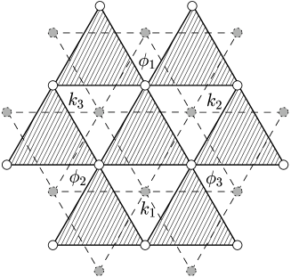
Figure 1: Triangular lattice and its dual (shown dashed). The up-pointing triangle surrounded by the variables $\phi_{1},\phi_{2},\phi_{3}$ is transformed into the down-pointing triangle surrounded by $k_{1},k_{2},k_{3}$.

The variable of summation is not written as the original $\phi_{i}$ but in terms of the directed difference $\phi_{ij}=\phi_{i}-\phi_{j}$ defined on each bond. This is possible if we introduce restrictions represented by the Kronecker deltas (which are defined with mod $q$) as in eq. (2) allocated to all up-pointing and down-pointing triangles. For instance, $\phi_{12}(=\phi_{1}-\phi_{2})$, $\phi_{23}(=\phi_{2}-\phi_{3})$, and $\phi_{31}(=\phi_{3}-\phi_{1})$ are not independent but satisfy $\phi_{12}+\phi_{23}+\phi_{31}=0$ (mod $q$), where 1, 2, and 3 are sites around the unit triangle as indicated in Fig. 1. The overall factor $q$ on the right hand side of eq. (2) reflects the invariance of the system under the uniform change $\phi_{i}\to\phi_{i}+l~{}(\forall i,0\leq l\leq q-1)$.

It is convenient to Fourier-transform the Kronecker deltas for down-pointing triangles and allocate the resulting exponential factors to the edges of three neighbouring up-pointing triangles. Then the partition function can be written only in terms of a product over up-pointing triangles:

$$Z=q\sum_{\{k_{i}\}}\sum_{\{\phi_{ij}\}}\prod_{\bigtriangleup}\left[\frac{1}{q}A[\phi_{12},\phi_{23},\phi_{31}]\delta(\phi_{12}+\phi_{23}+\phi_{31})\exp\left\{\frac{2\pi i}{q}(k_{1}\phi_{23}+k_{2}\phi_{31}+k_{3}\phi_{12})\right\}\right],$$ (3)

where $A[\phi_{12},\phi_{23},\phi_{31}]=x[\phi_{12}]x[\phi_{23}]x[\phi_{31}]$.

Now let us regard the product over up-pointing triangles in eq. (3) as a product over down-pointing triangles overlaying the original up-pointing triangles as shown dashed in Fig. 1. This viewpoint allows us to regard the quantity in the square brackets of eq. (3) as the Boltzmann factor for the unit triangle (to be called the face Boltzmann factor hereafter) of the dual triangular lattice composed of overlaying down-pointing triangles:

$$Z=q\sum_{\{k_{i}\}}\prod_{\bigtriangledown^{*}}A^{*}[k_{12},k_{23},k_{31}],$$ (4)

where

$$A^{*}[k_{12},k_{23},k_{31}] = \frac{1}{q}\sum_{\phi_{12},\phi_{23},\phi_{31}=0}^{q-1}A[\phi_{12},\phi_{23},\phi_{31}]\delta(\phi_{12}+\phi_{23}+\phi_{31})$$ (5)

$$\times\exp\left\{\frac{2\pi i}{q}(k_{1}\phi_{23}+k_{2}\phi_{31}+k_{3}\phi_{12})\right\}.$$

Here we have used the fact that the right hand side is a function of the differences $k_{i}-k_{j}\equiv k_{ij}~{}((ij)=(12),(23),(31))$ due to the constraint $\phi_{12}+\phi_{23}+\phi_{31}=0$.

This is a duality relation which exchanges the original model on the triangular lattice with a dual system on the dual triangular lattice. $A^{*}[k_{12},k_{23},k_{31}]$ represents the face Boltzmann factor of the dual system, which is the function of the differences between the nearest neighbor sites on the unit triangles similarly to face Boltzmann factor $A[\phi_{12},\phi_{23},\phi_{31}]$ of the original system.

It is easy to verify that the usual duality relation for the triangular lattice emerges from the present formulation. As an example, the ferromagnetic Ising model on the triangular lattice has the following face Boltzmann factors:

$$A[0,0,0]={\rm e}^{3K},~{}~{}A[1,1,0]=A[1,0,1]=A[0,1,1]={\rm e}^{-K},\cdots,$$ (6)

where $A[0,0,0]$ is for the all-parallel neighbouring spin configuration for three edges of a unit triangle, and $A[1,1,0]$ is for two antiparallel pairs and a single parallel pair around a unit triangle. The dual are, according to eq. (5),

$$A^{*}[0,0,0]=\frac{1}{2}\left\{A[0,0,0]+3A[1,1,0]\right\},~{}A^{*}[1,1,0]=\frac{1}{2}\left\{A[0,0,0]-A[1,1,0]\right\}.$$ (7)

It then follows that

$${\rm e}^{-4K^{*}}\equiv\frac{A^{*}[1,1,0]}{A^{*}[0,0,0]}=\frac{1-{\rm e}^{-4K}}{1+3{\rm e}^{-4K}}.$$ (8)

This formula is equivalent to the expression obtained by the ordinary duality, which relates the triangular lattice to the hexagonal lattice, followed by the star-triangle transformation:

$$(1+3{\rm e}^{-4K})(1+3{\rm e}^{-4K^{*}})=4.$$ (9)

3 Replicated system

It is straightforward to generalize the formulation of the previous section to the spin glass model using the replica method. The duality relation for the face Boltzmann factor of the replicated system is

$$A^{*}[\{k_{12}^{\alpha}\},\{k_{23}^{\alpha}\},\{k_{31}^{\alpha}\}] = \frac{1}{q^{n}}\sum_{\{\phi\}}\left[\prod_{\alpha=1}^{n}\delta(\phi_{a}^{\alpha}+\phi_{b}^{\alpha}+\phi_{c}^{\alpha})\right]A\left[\{\phi_{a}^{\alpha}\},\{\phi_{b}^{\alpha}\},\{\phi_{c}^{\alpha}\}\right]$$ (10)

$$\times\exp\left\{\frac{2\pi i}{q}\sum_{\alpha=1}^{n}(k_{1}^{\alpha}\phi_{b}^{\alpha}+k_{2}^{\alpha}\phi_{c}^{\alpha}+k_{3}^{\alpha}\phi_{a}^{\alpha})\right\},$$

where $\alpha$ is the replica index running from 1 to $n$, $\{k_{ij}^{\alpha}\}$ denotes the set $\{k_{ij}^{1},k_{ij}^{2},\cdots,k_{ij}^{n}\}$, and similarly for $\{\phi_{a}^{\alpha}\}$ etc. The variables $\phi_{a}^{\alpha},\phi_{b}^{\alpha},\phi_{c}^{\alpha}$ correspond to $\phi_{12},\phi_{23},\phi_{31}$ in eq. (3). The original face Boltzmann factor is the product of three edge Boltzmann factors

$$A\left[\{\phi_{a}^{\alpha}\},\{\phi_{b}^{\alpha}\},\{\phi_{c}^{\alpha}\}\right]=\chi_{\phi_{a}^{1}\cdots\phi_{a}^{n}}\cdot\chi_{\phi_{b}^{1}\cdots\phi_{b}^{n}}\cdot\chi_{\phi_{c}^{1}\cdots\phi_{c}^{n}},$$ (11)

where $\chi_{\phi^{1}\cdots\phi^{n}}$ is the averaged edge Boltzmann factor

$$\chi_{\phi^{1}\cdots\phi^{n}}=\sum_{l=0}^{q-1}p_{l}\,x[\phi^{1}+l]x[\phi^{2}+l]\cdots x[\phi^{n}+l].$$ (12)

Here $p_{l}$ is the probability that the relative value of neighbouring spin variables is shifted by $l$. A simple example is the $\pm J$ Ising model ($q=2$), in which $p_{0}=p$ (ferromagnetic interaction) and $p_{1}=1-p$ (antiferromagnetic interaction).

The average of the replicated partition function $Z_{n}$ is a function of face Boltzmann factors for various values of $\phi$’s. The triangular-triangular duality relation is then written as[5, 6, 7]

$$Z_{n}(A[\{0\},\{0\},\{0\}],\cdots)=cZ_{n}(A^{*}[\{0\},\{0\},\{0\}],\cdots),$$ (13)

where $c$ is a trivial constant and $\{0\}$ denotes the set of $n$ 0’s. Since eq. (13) is a duality relation for a multivariable function, it is in general impossible to identify the singularity of the system with the fixed point of the duality transformation. Nevertheless, it has been firmly established in simpler cases (such as the square lattice) that the location of the multicritical point in the phase diagram of spin glasses can be predicted very accurately, possibly exactly, by using the fixed-point condition of the principal Boltzmann factor for all-parallel configuration $\{0\}$. [4, 5, 6, 7] We therefore try the ansatz also for the triangular lattice that the exact location of the multicritical point of the replicated system is given by the fixed-point condition of the principal face Boltzmann factor:

$$A\left[\{0\},\{0\},\{0\}\right]=A^{*}\left[\{0\},\{0\},\{0\}\right],$$ (14)

combined with the Nishimori line (NL) condition, on which the multicritical point is expected to lie [9, 10].

For simplicity, we restrict ourselves to the $\pm J$ Ising model hereafter. Then the NL condition is ${\rm e}^{-2K}=(1-p)/p$, where $p$ is the probability of ferromagnetic interaction. The original face Boltzmann factor is a simple product of three edge Boltzmann factors,

$$A\left[\{0\},\{0\},\{0\}\right]=\chi_{0}^{3}$$ (15)

with

$$\chi_{0}=p{\rm e}^{nK}+(1-p){\rm e}^{-nK}=\frac{{\rm e}^{(n+1)K}+{\rm e}^{-(n+1)K}}{{\rm e}^{K}+{\rm e}^{-K}}.$$ (16)

The dual Boltzmann factor $A^{*}[\{0\},\{0\},\{0\}]$ needs a more elaborate treatment. The constraint of Kronecker delta in eq. (10) may be expressed as

$$\prod_{\alpha=1}^{n}\delta(\phi_{a}^{\alpha}+\phi_{b}^{\alpha}+\phi_{c}^{\alpha})=2^{-n}\sum_{\{\tau_{\alpha}=0,1\}}\exp\left[\pi i\sum_{\alpha=1}^{n}\tau_{\alpha}(\phi_{a}^{\alpha}+\phi_{b}^{\alpha}+\phi_{c}^{\alpha})\right].$$ (17)

The face Boltzmann factor $A\left[\{\phi_{a}^{\alpha}\},\{\phi_{b}^{\alpha}\},\{\phi_{c}^{\alpha}\}\right]$ is the product of three edge Boltzmann factors, each of which may be written as, on the NL, [7]

$$\chi_{\phi_{a}^{1}\cdots\phi_{a}^{n}} = p\exp\left[\sum_{\alpha=1}^{n}(1-2\phi_{a}^{\alpha})K\right]+(1-p)\exp\left[-\sum_{\alpha=1}^{n}(1-2\phi_{a}^{\alpha})K\right]$$ (18)

$$= \frac{1}{2\cosh K}\sum_{\eta_{a}=\pm 1}\exp\left[\eta_{a}K+\eta_{a}K\sum_{\alpha=1}^{n}(1-2\phi_{a}^{\alpha}K)\right].$$

Using eqs. (17) and (18), eq. (10) can be rewritten as, for the principal Boltzmann factor with all $k_{i}^{\alpha}=0$,

$$A^{*}\left[\{0\},\{0\},\{0\}\right]=\frac{1}{4^{n}(2\cosh K)^{3}}\sum_{\eta}\sum_{\tau}\sum_{\phi}\exp\left[\pi i\sum_{\alpha}\tau_{\alpha}(\phi_{a}^{\alpha}+\phi_{b}^{\alpha}+\phi_{c}^{\alpha})\right.$$

$$+\left.K(\eta_{a}+\eta_{b}+\eta_{c})+K\eta_{a}\sum_{\alpha}(1-2\phi_{a}^{\alpha})+K\eta_{b}\sum_{\alpha}(1-2\phi_{b}^{\alpha})+K\eta_{c}\sum_{\alpha}(1-2\phi_{c}^{\alpha})\right].$$ (19)

The right hand side of this equation can be evaluated explicitly as shown in the Appendix. The result is

$$A^{*}\left[\{0\},\{0\},\{0\}\right]=4^{-n}(2\cosh K)^{3n-3}$$

$$\times\left[({\rm e}^{3K}+3{\rm e}^{-K})(1+\tanh^{3}K)^{n}+(3{\rm e}^{K}+{\rm e}^{-3K})(1-\tanh^{3}K)^{n}\right].$$ (20)

The prescription (14) for the multicritical point is therefore

$$\frac{\cosh^{3}(n+1)K}{\cosh^{3}K}=\frac{(2\cosh K)^{3n}}{4^{n}(2\cosh K)^{3}}$$

$$\times\left[({\rm e}^{3K}+3{\rm e}^{-K})(1+\tanh^{3}K)^{n}+(3{\rm e}^{K}+{\rm e}^{-3K})(1-\tanh^{3}K)^{n}\right].$$ (21)

4 Multicritical point

The conjecture (21) for the exact location of the multicritical point can be verified for $n=1,2$ and $\infty$ since these cases can be treated directly without using the above formulation.

The case $n=1$ is an annealed system and the problem can be solved explicitly. It is easy to show that the annealed $\pm J$ Ising model is equivalent to the ferromagnetic Ising model with effective coupling $\tilde{K}$ satisfying

$$\tanh\tilde{K}=(2p-1)\tanh K.$$ (22)

If we insert the transition point of the ferromagnetic Ising model on the triangular lattice ${\rm e}^{4\tilde{K}}=3$, eq. (22) reads

$$(2p-1)\tanh K=2-\sqrt{3}.$$ (23)

This formula represents the exact phase boundary for the annealed system. Under the NL condition, it is straightforward to verify that this expression agrees with the conjectured multicritical point of eq. (21). It is indeed possible to show further that the whole phase boundary of eq. (23) can be derived by evaluating $A^{*}[0,0,0]$ directly for $n=1$ for arbitrary $p$ and $K$, giving $2A^{*}[0,0,0]=\chi_{0}^{3}+3\chi_{1}^{2}\chi_{0}$ with $\chi_{0}=p{\rm e}^{K}+(1-p){\rm e}^{-K},\chi_{1}=p{\rm e}^{-K}+(1-p){\rm e}^{K}$, and using the condition $A^{*}[0,0,0]=A[0,0,0]$.

When $n=2$, a direct evaluation of the edge Boltzmann factor reveals that the system on the NL is a four-state Potts model with effective coupling $\tilde{K}$ satisfying [7, 5]

$${\rm e}^{\tilde{K}}={\rm e}^{2K}-1+{\rm e}^{-2K}.$$ (24)

Since the transition point of the non-random four-state Potts model on the triangular lattice is given by ${\rm e}^{\tilde{K}}=2$ [8], the (multi)critical point of the $n=2$ system is specified by the relation

$${\rm e}^{2K}-1+{\rm e}^{-2K}=2.$$ (25)

Equation (21) with $n=2$ also gives this same expression, which confirms validity of our conjecture in the present case as well.

The limit $n\to\infty$ can be analyzed as follows.[5] The average of the replicated partition function

$$[Z^{n}]_{\rm av}=[{\rm e}^{-n\beta F}]_{\rm av},$$ (26)

where $[\cdots]_{\rm av}$ denotes the configurational average, is dominated in the limit $n\to\infty$ by contributions from bond configurations with the smallest value of the free energy $F$. It is expected that the bond configurations without frustration (i.e., ferromagnetic Ising model and its gauge equivalents) have the smallest free energy, and therefore we may reasonably expect that the $n\to\infty$ systems is described by the non-random model. Thus the critical point is given by ${\rm e}^{4K}=3$. It is straightforward to check that eq. (21) reduces to the same equation in the limit $n\to\infty$.

These analyses give us a good motivation to apply eq. (21) to the quenched limit $n\to 0$. Expanding eq. (21) around $n=0$, we find, from the coefficients of terms linear in $n$,

$$3K\tanh K = 3\log(2\cosh K)-\log 4$$ (27)

$$+\frac{{\rm e}^{3K}+3{\rm e}^{-K}}{(2\cosh K)^{3}}\log(1+\tanh^{3}K)+\frac{3{\rm e}^{K}+{\rm e}^{-3K}}{(2\cosh K)^{3}}\log(1-\tanh^{3}K),$$

or, in terms of $p$, using ${\rm e}^{-2K}=(1-p)/p$,

$$2p^{2}(3-2p)\log p+2(1-p)^{2}(1+2p)\log(1-p)+\log 2$$

$$=p(4p^{2}-6p+3)\log(4p^{2}-6p+3)+(1-p)(4p^{2}-2p+1)\log(4p^{2}-2p+1).$$ (28)

Equation (28) is our conjecture for the exact location of the multicritical point $p_{\rm c}$ of the $\pm J$ Ising model on the triangular lattice. This gives $p_{\rm c}=0.8358058$, which agrees well with a recent high-precision numerical estimate, 0.8355(5) [11].

If we further use the conjecture [7] $H(p_{\rm c})+H(p_{\rm c}^{\prime})=1$, where $H(p)$ is the binary entropy $-p\log_{2}p-(1-p)\log_{2}(1-p)$, to relate this $p_{\rm c}$ with that for the hexagonal lattice $p_{\rm c}^{\prime}$, we find $p_{\rm c}^{\prime}=0.9327041$. Again, the numerical result 0.9325(5) [11] is very close to this conclusion.

5 Conclusion

To summarize, we have formulated the duality transformation of the replicated random system on the triangular lattice, which brings the triangular lattice to a dual triangular lattice without recourse to the hexagonal lattice. The result was used to predict the exact location of the multicritical point of the $\pm J$ Ising model on the triangular lattice. Correctness of our theory has been confirmed in directly solvable cases of $n=1,2$ and $\infty$. Application to the quenched limit $n\to 0$ yielded a value in impressive agreement with a numerical estimate.

The status of our result for the quenched system, eq. (28), is a conjecture for the exact solution. It is difficult at present to prove this formula rigorously. This is the same situation as in cases for other lattices and models [4, 5, 6, 7]. We nevertheless expect that such a proof should be eventually possible since a single unified theoretical framework always gives results in excellent agreement with independent numerical estimations for a wide range of systems. Further efforts toward a formal proof are required.

Appendix

In this Appendix we evaluate eq. (19) to give eq. (20). Let us denote $4^{n}(2\cosh K)^{3}A^{*}[\{0\},\{0\},\{0\}]$ as $\tilde{A}$. The sums over $\alpha$ in the exponent of eq. (19) can be expressed as the product over $\alpha$:

$$\tilde{A} = \sum_{\eta}{\rm e}^{K(n+1)(\eta_{a}+\eta_{b}+\eta_{c})}$$ (29)

$$\times \prod_{\alpha=1}^{n}\left[\sum_{\tau_{\alpha}=0}^{1}\left(\sum_{\phi_{a}^{\alpha}=0}^{1}{\rm e}^{\pi i\tau_{\alpha}\phi_{a}^{\alpha}-2K\eta_{a}\phi_{a}^{\alpha}}\sum_{\phi_{b}^{\alpha}=0}^{1}{\rm e}^{\pi i\tau_{\alpha}\phi_{b}^{\alpha}-2K\eta_{b}\phi_{b}^{\alpha}}\sum_{\phi_{c}^{\alpha}=0}^{1}{\rm e}^{\pi i\tau_{\alpha}\phi_{c}^{\alpha}-2K\eta_{c}\phi_{c}^{\alpha}}\right)\right].$$

By performing the sums over $\phi$ and $\tau$ for each replica, we find

$$\tilde{A} = \sum_{\eta_{a},\eta_{b},\eta_{c}=\pm 1}{\rm e}^{K(n+1)(\eta_{a}+\eta_{b}+\eta_{c})}\prod_{\alpha=1}^{n}\left[(1+{\rm e}^{-2K\eta_{a}})(1+{\rm e}^{-2K\eta_{b}})(1+{\rm e}^{-2K\eta_{c}})\right.$$ (30)

$$\left.+(1-{\rm e}^{-2K\eta_{a}})(1-{\rm e}^{-2K\eta_{b}})(1-{\rm e}^{-2K\eta_{c}})\right].$$

It is straightforward to write down the eight terms appearing in the above sum over $\eta_{a},\eta_{b},\eta_{c}$ to yield

$$\tilde{A} = {\rm e}^{3K(n+1)}\left[(1+{\rm e}^{-2K})^{3}+(1-{\rm e}^{-2K})^{3}\right]^{n}$$ (31)

$$+ 3{\rm e}^{K(n+1)}\left[(1+{\rm e}^{-2K})^{2}(1+{\rm e}^{2K})+(1-{\rm e}^{-2K})^{2}(1-{\rm e}^{2K})\right]^{n}$$

$$+ 3{\rm e}^{-K(n+1)}\left[(1+{\rm e}^{-2K})(1+{\rm e}^{2K})^{2}+(1-{\rm e}^{-2K})(1-{\rm e}^{2K})^{2}\right]^{n}$$

$$+ {\rm e}^{-3K(n+1)}\left[(1+{\rm e}^{2K})^{3}+(1-{\rm e}^{2K})^{3}\right]^{n},$$

which is further simplified into

$$\tilde{A} = {\rm e}^{3K}\left[(2\cosh K)^{3}+(2\sinh K)^{3}\right]^{n}$$ (32)

$$+ 3{\rm e}^{K}\left[(2\cosh K)^{3}-(2\sinh K)^{3}\right]^{n}$$

$$+ 3{\rm e}^{-K}\left[(2\cosh K)^{3}+(2\sinh K)^{3}\right]^{n}$$

$$+ {\rm e}^{-3K}\left[(2\cosh K)^{3}-(2\sinh K)^{3}\right]^{n}$$

$$= (2\cosh K)^{3n}$$

$$\times\left[({\rm e}^{3K}+3{\rm e}^{-K})(1+\tanh^{3}K)^{n}+(3{\rm e}^{K}+{\rm e}^{-3K})(1-\tanh^{3}K)^{n}\right].$$

This is eq. (20).

  The present version includes a few corrections in the notation and supersedes the published version, J. Phys. Soc. Jpn. 75 (2006) 034004.