Orientation selection in lamellar phases by oscillatory shears

Abstract

In order to address the selection mechanism that is responsible for the unique lamellar orientation observed in block copolymers under oscillatory shears, we use a constitutive law for the dissipative part of the stress tensor that respects the uniaxial symmetry of a lamellar phase. An interface separating two domains oriented parallel and perpendicular to the shear is shown to be hydrodynamically unstable, a situation analogous to the thin layer instability of stratified fluids under shear. The resulting secondary flows break the degeneracy between parallel and perpendicular lamellar orientation, leading to a preferred perpendicular orientation in certain ranges of parameters of the polymer and of the shear.

Oscillatory shears are often used to promote long range order in lamellar phases of block copolymers, yet the mechanisms responsible for selecting a particular lamellar orientation relative to the shear remain unknown. A possible mechanism based on a hydrodynamic instability in a microphase separated copolymer is presented here that can distinguish between the experimentally important cases of parallel and perpendicular orientations (Fig. 1). The instability occurs at the boundary separating parallel and perpendicular regions provided that the dissipative part of the stress tensor of the copolymer is chosen to reflect the uniaxial symmetry of these broken symmetry phases. Our results rely solely on the uniaxial symmetry of the microphases, and therefore should generally apply to other complex fluids of the same symmetry.

Block copolymers are being extensively investigated as nanoscale templates for a wide variety of applications that include nanolithography re:harrison00b ; re:black04 ; re:black05 , photonic components re:urbas99 , or high density storage systems re:thurn-albrecht00 . However, given the small wavelength of the microphases (tens or hundreds of Angstroms), macroscopic size samples do not completely order through spontaneous self assembly. Instead, oscillatory shears are commonly introduced in order to accelerate long range order development over the required distances (see Ref. re:larson99, for a recent review). In practice, a variety of lamellar orientations are observed depending on the architecture of the block and the parameters of the shear re:larson99 ; re:koppi92 ; re:patel95 ; re:maring97 ; re:leist99 ; re:chen98b , while the mechanisms responsible for orientation selection are not yet understood. The first theoretical analysis of orientation selection in block copolymers was conducted in the vicinity of the order-disorder transition of the copolymer, and addressed the effect of a steady shear on the growth of critical fluctuations re:cates89 . Fluctuations along the perpendicular orientation were shown to be less suppressed by the shear, and hence it was argued that this orientation would be selected. Consideration was later given to anisotropic viscosities of the microphases, which led to different relative stabilities of uniform parallel and perpendicular configurations due to the different effects of thermal fluctuations on each orientation re:goulian95 . Later work focused on the role played by viscosity contrast between the polymer blocks re:fredrickson94 , and showed that the perpendicular alignment dominates for high shear rates, and parallel otherwise. Existing experimental phenomenology concerning orientation selection is far more complex than these analyses would suggest, and is seen to drastically depend on the architecture of the block re:larson99 . The analysis that we present does not rely on fluctuation effects near critical points, allows for oscillatory shears, and explicitly incorporates hydrodynamic effects resulting from viscosity contrast between the microphases, thus overcoming the limitations of previous treatments.

The experimentally relevant range of shear frequencies is well below the inverse characteristic relaxation times of the polymer chains, and hence a reduced description in terms of the monomer volume fraction is adopted re:leibler80 ; re:ohta86 ; re:fredrickson94 . According to this description, the lamellar phase response is solid like or elastic for perturbations directed along the lamellae normal, and fluid like or viscous on the lamellar plane. In the limit of vanishing frequency, the viscous part of the response has been assumed to be Newtonian with uniform shear viscosity, and therefore parallel and perpendicular orientations are degenerate and unmodified by the shear. We address below the consequences of what we believe is the leading deviation away from Newtonian response in the limits of low frequency and characteristic flow scale much longer than the lamellar spacing: the viscous stress tensor of a lamellar phase is, by reason of symmetry, the same as that of any other uniaxial phase (e.g., a nematic liquid crystal re:martin72 ; re:degennes93 ). The slowly varying local wavevector of the lamellae plays a role analogous to that of the director in a nematic. The rest of this paper is devoted to the study of the effect of this assumption on the hydrodynamic stability of the configuration shown in Fig. 1.

We assume that the dissipative part of the linear stress tensor is that of a uniaxial, incompressible phase re:degennes93 ,

$$\sigma^{D}_{ij}=\eta D_{ij}+\alpha_{1}\hat{n}_{i}\hat{n}_{j}\hat{n}_{k}\hat{n}_{l}D_{kl}+\alpha_{56}(\hat{n}_{i}\hat{n}_{k}D_{jk}+\hat{n}_{j}\hat{n}_{k}D_{ik})$$ (1)

with $i,j,k=x,y,z$, $D_{ij}=\partial_{i}v_{j}+\partial_{j}v_{i}$ with $v_{i}$ the local velocity field, and $\hat{\mathbf{n}}=(\hat{n}_{x},\hat{n}_{y},\hat{n}_{z})$ denoting the slowly varying normal to the lamellar planes. The Newtonian viscosity is $\eta$, and $\alpha_{1}$ and $\alpha_{56}$ are two independent viscosity coefficients. The dynamic viscosity $\eta^{\prime}$ ($\eta^{\prime}=G^{\prime\prime}/\omega$, with $G^{\prime\prime}$ the loss modulus and $\omega$ the shear frequency) is $\eta^{\prime}=\eta$ for a fully ordered perpendicular configuration ($\hat{\mathbf{n}}=(1,0,0)$), and $\eta^{\prime}=\eta+\alpha_{56}$ for a parallel orientation ($\hat{\mathbf{n}}=(0,0,1)$). This model is consistent with low frequency rheology in PEP-PEE diblocks showing $\eta^{\prime}_{\rm par}>\eta^{\prime}_{\rm perp}$ re:koppi92 if $\alpha_{56}>0$, and with PS-PI diblocks $\eta^{\prime}_{\rm par}<\eta^{\prime}_{\rm perp}$ re:chen98b if $\alpha_{56}<0$. Given this assumption, the effective dynamic viscosity in the two domain configuration of Fig. 1 would be different in each domain. It is known that the analogous configuration for the case of two Newtonian fluids of different viscosity is unstable both for steady re:yih67 ; re:hooper85 and oscillatory re:king99 shears. We describe below the extension of these results to uniaxial phases in the limit of small but nonzero Reynolds number flows.

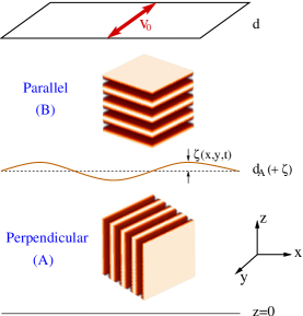
Figure 1: Schematic representation of a parallel/perpendicular configuration begin sheared along $\hat{y}$.

We consider a base state involving perpendicular (A) and parallel (B) regions separated by a planar surface, subjected to an imposed shear ${\mathbf{v}}_{0}=\gamma\omega d\cos(\omega t)\hat{\mathbf{y}}$ at $z=d$, and ${\mathbf{v}}_{0}=0$ at $z=0$ (Fig. 1), with $\gamma$ the shear amplitude and $d$ the system thickness. The resulting velocity field ${\mathbf{v}}_{A,B}=(0,V_{A,B},0)$ is the same as that of two superposed Newtonian fluids with viscosities $\mu_{A}=\eta$ and $\mu_{B}=\eta+\alpha_{56}$. We then consider a small perturbation of the domain boundary as shown in Fig. 1, and write the velocity fields in A and B as $v_{i}^{A,B}=V_{A,B}\delta_{iy}+u_{i}^{A,B}$ ($i=x,y,z$). By expanding $u_{i}^{A,B}=\sum_{q_{x},q_{y}}\hat{u}_{i}^{A,B}(q_{x},q_{y},z,t)\exp[i(q_{x}x+q_{y}y)]$, substituting into the modified Navier Stokes equation that results from the choice of Eq. (1), linearizing, and eliminating pressure and $\hat{u}_{y}$, we find

$$Re\left[(\partial_{t}+iq_{y}V_{A})(\partial_{z}^{2}-q^{2})\hat{u}_{z}^{A}-iq_{y}(\partial_{z}^{2}V_{A})\hat{u}_{z}^{A}\right]$$

$$=(\partial_{z}^{2}-q^{2})^{2}\hat{u}_{z}^{A}-\alpha_{56}q_{x}^{2}(\partial_{z}^{2}-q^{2})\hat{u}_{z}^{A}$$

$$+iq_{x}[2\alpha_{1}q_{x}^{2}-\alpha_{56}(\partial_{z}^{2}-q^{2})]\partial_{z}\hat{u}_{x}^{A},$$ (2)

$$Re\left[\partial_{t}(\partial_{z}^{2}-q^{2})\hat{u}_{x}^{A}+iq_{y}(\partial_{z}^{2}-q^{2})(V_{A}\hat{u}_{x}^{A})+\right.$$

$$\left.2q_{x}q_{y}(\partial_{z}V_{A})\hat{u}_{z}^{A}\right]=(1+\alpha_{56})(\partial_{z}^{2}-q^{2})^{2}\hat{u}_{x}^{A}$$

$$-2\alpha_{1}q_{x}^{2}(\partial_{z}^{2}-q_{y}^{2})\hat{u}_{x}^{A},$$ (3)

for the perpendicular domain A ($0\leq z\leq d_{A}$). Here $q^{2}=q_{x}^{2}+q_{y}^{2}$ and $Re=\rho\omega d^{2}/\eta$ is the Reynolds number, with $\rho$ the copolymer density. Similarly

$$Re\left[(\partial_{t}+iq_{y}V_{B})(\partial_{z}^{2}-q^{2})\hat{u}_{z}^{B}-iq_{y}(\partial_{z}^{2}V_{B})\hat{u}_{z}^{B}\right]$$

$$=(1+\alpha_{56})(\partial_{z}^{2}-q^{2})^{2}\hat{u}_{z}^{B}-2\alpha_{1}q^{2}\partial_{z}^{2}\hat{u}_{z}^{B},$$ (4)

$$Re\left[\partial_{t}(\partial_{z}^{2}-q^{2})\hat{u}_{x}^{B}+iq_{y}(\partial_{z}^{2}-q^{2})(V_{B}\hat{u}_{x}^{B})+\right.$$

$$\left.2q_{x}q_{y}(\partial_{z}V_{B})\hat{u}_{z}^{B}\right]=(\partial_{z}^{2}-q^{2})^{2}\hat{u}_{x}^{B}$$

$$+\alpha_{56}(\partial_{z}^{2}-q^{2})\left(\partial_{z}^{2}\hat{u}_{x}^{B}-iq_{x}\partial_{z}\hat{u}_{z}^{B}\right)-2iq_{x}\alpha_{1}\partial_{z}^{3}\hat{u}_{z}^{B},$$ (5)

for the parallel region B ($d_{A}\leq z\leq d$). All quantities have been made dimensionless by a length scale $d$, a time scale $\omega^{-1}$, and rescaling viscosities by $\eta$, i.e., $\alpha_{1}\rightarrow\alpha_{1}/\eta$ and $\alpha_{56}\rightarrow\alpha_{56}/\eta$ ($\mu_{A}=1$, $\mu_{B}=1+\alpha_{56}$). Rigid boundary conditions are used on the planes $z=0$ and $z=d$ ($d=1$ after rescaling). At the interface $z=d_{A}+\zeta(x,y,t)$ we have ${\mathbf{v}}^{A}={\mathbf{v}}^{B}$, and $(\sigma_{ij}^{B}-\sigma_{ij}^{A})\hat{n}_{j}=-\Gamma^{\prime}(\partial_{x}^{2}+\partial_{y}^{2})\zeta\hat{n}_{i}\delta_{iz}$ with $\Gamma^{\prime}=\Gamma/(\eta\omega d)$ and $\Gamma$ the interfacial tension. Also, the kinematic boundary condition for the interface is $\left(\partial_{t}+{\mathbf{v}}^{B}\cdot{\mathbf{\nabla}}\right)\zeta=v_{z}^{B}$.

Equations (2)–(5) are similar to the Orr-Sommerfeld equation for the Newtonian case re:yih67 ; re:hooper85 ; re:king99 , except that $x$ and $z$ velocity fields are now coupled (except at $q_{x}=0$). The solution can be found by writing $\hat{u}_{z,x}^{A,B}=\exp(\sigma t)\phi_{z,x}^{A,B}$ and $\hat{\zeta}=\exp(\sigma t)h$, with $\hat{\zeta}$ the Fourier transform of $\zeta$, and $\sigma$ the Floquet exponent yielding the perturbation growth rate (coefficients in Eqs. (2)–(5) proportional to $V_{A,B}$ are periodic in time).

For typical block copolymers, $\rho\sim 1$ g cm^-3, $d\sim 1$ cm, and $\eta\sim 10^{4}$–$10^{6}$ P, resulting in $Re/\omega=10^{-4}$–$10^{-6}$ s. Hence $Re\ll 1$ for the frequencies of interest. We further expand the velocity, interfacial functions $\phi_{z,x}^{A,B}$, $h$, as well as the Floquet exponent $\sigma$ in powers of $Re$, and solve Eqs. (2)–(5) order by order. In the limit $Re\rightarrow 0$ while keeping the surface tension $\Gamma^{\prime}$ finite, we find $\sigma=f_{z0}^{B}(q_{x},q_{y})\Gamma^{\prime}$, with $f_{z0}^{B}<0$ for all wave numbers $q_{x}$ and $q_{y}$. Hence the interface is stable, indicating coexistence of parallel and perpendicular orientations in this limit.

The situation is different for small but finite values of $Re$. In this case we need to address the order of $\Gamma^{\prime}$ as well. Typical values of $\Gamma\sim 1$ dyne/cm lead to $\Gamma^{\prime}\omega=10^{-4}$–$10^{-6}$ s^-1. Given that $Re/\omega=10^{-4}$–$10^{-6}$ s, and that $\omega\sim 1$ s^-1 in typical experiments, we consider the distinguished limit $\Gamma^{\prime}={\cal O}(Re)$. Writing $\Gamma^{\prime}=\Gamma_{1}Re$, and $\sigma=\sigma_{1}Re$, we find

$$\sigma_{1}=f_{z0}^{B}(q_{x},q_{y})\Gamma_{1}+\frac{1}{2}\delta^{2}\gamma^{2}f_{z1}^{B}(q_{x},q_{y}).$$ (6)

Here $\delta=m\lambda_{0}$ is proportional to the viscosity contrast $m=\mu_{A}/\mu_{B}$, with $\lambda_{0}=(d_{A}+md_{B})^{-1}$, $d_{B}=d-d_{A}$, and the function $f_{z1}^{B}(q_{x},q_{y})$ depends on the system parameters $\alpha_{1}$, $\alpha_{56}$, and on $d_{A}$, but not on the shear parameters $\gamma$ and $\omega$. Whereas $f_{z0}^{B}$ is always negative, $f_{z1}^{B}$ can be positive so that Eq. (6) illustrates the competition between the stabilizing effect of surface tension and the destabilizing effect of the imposed shear flow. Note that $\Gamma_{1}$ can be written as $\Gamma_{1}=1/We=\theta\omega^{-2}$, with $We$ the Weber number and $\theta=\Gamma/(\rho d^{3})$. Thus, we have $\sigma_{1}=\sigma_{1}(\gamma^{2},\omega^{-2})$, and instability is increased at large shear amplitudes and frequencies.

Typical results for $\sigma$ as a function of wave vector are shown in Fig. 2. Unstable wave vectors are near $q_{x}=0$. This indicates the absence of interfacial modulation along the $x$ direction (the transverse direction for perpendicular lamellae), and $u_{x}=0$ for the associated velocity perturbations. We have repeated the calculations for different ranges of parameters, and found similar results for both $\sigma$ and velocity perturbations.

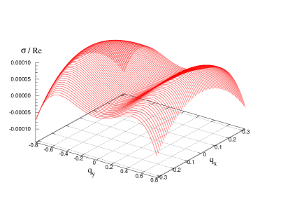
Figure 2: Growth rate $\sigma/Re$ as a function of wave numbers $q_{x}$ and $q_{y}$, for $\alpha_{1}=1$, $\alpha_{56}=-0.9$, $\gamma=1$, $Re=5\times 10^{-4}$, and $d_{A}=1/2$. The maximum growth rate is found at $q_{x}^{\rm max}=0$, $q_{y}^{\rm max}=\pm 0.61$.

Based on these results, further progress in determining the stability boundary can be made by examining only long waves along the $y$ direction (with $q=q_{y}$). Equation (6) can be expanded as $f_{z0}^{B}=-f_{0}q^{4}+{\cal O}(q^{6})$, $f_{z1}^{B}=f_{1}q^{2}+f_{2}q^{4}+{\cal O}(q^{6})$, so that the Floquet exponent can be rewritten as

$$\sigma_{1}=\frac{1}{2}\delta^{2}\gamma^{2}f_{1}q^{2}-(\theta f_{0}\omega^{-2}-\frac{1}{2}\delta^{2}\gamma^{2}f_{2})q^{4},$$ (7)

where $f_{0}>0$ always, as noted above. Both $f_{1}=f_{1}(\alpha_{56},d_{A})$ and $f_{2}=f_{2}(\alpha_{1},\alpha_{56},d_{A})$ are complicated but known functions of their arguments. For small $q$ stability is determined by the sign of $f_{1}$ which depends on $\alpha_{56}$ and layer thickness $d_{A}$, but is independent of shear parameters. The calculated stability diagram in the $(d_{A}/d_{B},\mu_{B})$ plane ($\mu_{B}=1+\alpha_{56}$) is shown in Fig. 3. Note the symmetry under $d_{A}/d_{B}\rightarrow(d_{A}/d_{B})^{-1}$ and $\mu_{B}\rightarrow\mu_{B}^{-1}$ which suggests that this instability is related to the known two fluid instability produced by viscosity stratification re:hooper85 : instability occurs when the thinner domain is more viscous. In the present case, however, viscosity contrast between the domains is not caused by fluid stratification, but rather because of the effective viscosity contrast between lamellae of different orientations.

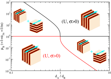
Figure 3: Orientation selection for uniaxial systems under oscillatory shear as a function of the layer thickness ratio and viscosity contrast. (U, $\sigma>0$) denotes the range in which the parallel orientation is unstable, leading to the selection of the perpendicular orientation.

The stability analysis discussed thus far is purely of hydrodynamic nature, but can we used to argue that growth of unstable modes above threshold leads to orientation selection. As can be seen from Fig. 1, parallel lamellae are marginal to velocity fields along $x$ and $y$ directions, but will be compressed or expanded by nonuniform flows along the $z$-direction. Conversely, perpendicular lamellae will be distorted by nonuniform flows along $x$, but not by flows along either $y$ or $z$. Since the instability mode is dominated by a velocity field along $z$, it will lead to weak and oscillatory compression and expansion of the parallel region, while leaving the perpendicular lamellae unaffected. The response of an interface separating two lamellar phases, subjected to periodic expansion and compression and the other marginal, has already been addressed in Ref. re:huang03, . We showed that the overall free energy of the system is reduced by the motion of the interface towards the distorted phase (which is storing elastic energy during each cycle of the shear) or, in the present case, toward the parallel region. In summary, Fig. 3 shows the regions of parameters in which parallel and perpendicular layers would coexist, and those in which the layer of perpendicular orientation would grow at the expense of the parallel layer. It would be interesting to test our predictions by examining a system comprising only two layers of different orientations and with varying ratios $d_{A}/d_{B}$ to directly address the stability of the configuration under shear, and to indirectly measure the coefficient $\alpha_{56}$ from the location of the instability threshold.

Experiments addressing orientation selection always involve coarsening of polycrystalline samples with a distribution of grain sizes, and hence a range of ratios $d_{A}/d_{B}$, and a distribution of orientations. It is generally argued that lamellar domains with local wavevector not on the parallel/perpendicular plane will be eliminated from the distribution rather quickly, and hence that the selection of a final orientation will be determined by the competition between parallel and perpendicular domains. Generally speaking, our results imply selection of the perpendicular orientation for finite shear frequencies and $\alpha_{56}>0$, the latter case appropriate for PEP-PEE but not PS-PI blocks if our assumption in Eq. (1) holds. If $\alpha_{56}<0$, Fig. 3 would suggest that a smaller than average layer of perpendicular orientation first grows at the expense of neighboring parallel layers. Following this initial coarsening in which $d_{A}/d_{B}$ increases in time, the stability boundary in this figure would be reached. It is difficult to assess in this case the impact of other dynamical factors affecting coarsening such as the effect of an already moving boundary and the concomitant flows, or spatial correlations built into the distribution of orientations following this intermediate coarsening re:mullins93 . In summary, if $\alpha_{56}<0$, as well as in the limit of $Re\rightarrow 0$, our study indicates coexistence of parallel and perpendicular domains, not inconsistently with experiments addressing orientation selection that indicate dependence on processing history or experimental details re:larson99 ; re:patel95 ; re:maring97 (e.g., quenched or annealed history of the sample, and the starting time of shear alignment).

Once within the region of instability, it is instructive to analyze the dependence of the growth rate of the most unstable perturbation on the parameters of the shear. This growth rate is given by $\sigma_{1}^{\rm max}=(\delta^{4}f_{1}^{2}/16f^{\prime})\gamma^{4}\omega^{2}$, with $f^{\prime}=\theta f_{0}-\delta^{2}f_{2}\gamma^{2}\omega^{2}/2$, and the corresponding most unstable wavenumber is $q_{\rm max}=\delta(f_{1}/f^{\prime})^{1/2}\gamma\omega/2$, both of which increase with shear amplitude and frequency. By noting that $\sigma_{1}^{\rm max}=\sigma_{\rm max}/Re=\sigma_{\rm max}\eta/(\rho d^{2}\omega)$, and that usually $\sigma_{\rm max}\ll(\rho d^{2}\delta^{2}f_{1}^{2}/8|f_{2}|\eta)\gamma^{2}\omega$ for small enough $\sigma_{\rm max}$, we find the maximum growth rate to be given by

$$\sigma_{\rm max}=\frac{\rho d^{2}\delta^{4}f_{1}^{2}}{16\theta f_{0}\eta}\gamma^{4}\omega^{3}.$$ (8)

Therefore, perturbation growth for a given block copolymer is constant along the line $\gamma\omega^{3/4}=$const. To our knowledge, the only experimental determination of the boundary in parameter space separating regions in which parallel or perpendicular lamellae are selected has been given for PS-PI copolymers re:maring97 ; re:leist99 . From a limited data set, it was approximated by $\gamma\omega=$ const. Since it is not inconceivable that the experimentally determined boundary does not correspond to the true stability boundary, but rather to the line in which $\sigma_{\rm max}$ becomes experimentally observable re:zf4 , it would be desirable to conduct the experiment in a block copolymer with $\alpha_{56}>0$.

In summary, by assuming that the dissipative part of the linear stress tensor of a block copolymer has to respect the broken symmetry of uniaxial lamellar phases, we have obtained a long wavelength hydrodynamic instability of the interface separating lamellae of parallel and perpendicular orientations under an imposed oscillatory shear. The instability leads to nonuniform secondary flows, which would favor the perpendicular orientation in large regions of parameter space. Since our results follow from the symmetry of the microphases, we would expect them to hold in other complex fluids of the same symmetry.

This research has been supported by the National Science Foundation under grant DMR-0100903, and by NSERC Canada.

References

- (1) C. Harrison et al., Science 290, 1558 (2000).
- (2) C. T. Black and O. Bezencenet, IEEE Trans. Nanotech. 3, 412 (2004).
- (3) C. T. Black, Appl. Phys. Lett. 87, 163116 (2005).
- (4) A. Urbas, Y. Fink, and E. L. Thomas, Macromolecules 32, 4748 (1999).
- (5) T. Thurn-Albrecht et al., Science 290, 5499 (2000).
- (6) R. G. Larson, The Structure and Rheology of Complex Fluids (Oxford University Press, New York, 1999).
- (7) K. A. Koppi et al., J. Phys. II (France) 2, 1941 (1992).
- (8) S. S. Patel, R. G. Larson, K. I. Winey, and H. Watanabe, Macromolecules 28, 4313 (1995).
- (9) D. Maring and U. Wiesner, Macromolecules 30, 660 (1997).
- (10) H. Leist, D. Maring, T. Thurn-Albrecht, and U. Wiesner, J. Chem. Phys. 110, 8225 (1999).
- (11) Z. R. Chen and J. A. Kornfield, Polymer 39, 4679 (1998).
- (12) M. E. Cates and S. T. Milner, Phys. Rev. Lett. 62, 1856 (1989).
- (13) M. Goulian and S. T. Milner, Phys. Rev. Lett. 74, 1775 (1995).
- (14) G. H. Fredrickson, J. Rheol. 38, 1045 (1994).
- (15) L. Leibler, Macromolecules 13, 1602 (1980).
- (16) T. Ohta and K. Kawasaki, Macromolecules 19, 2621 (1986).
- (17) P. C. Martin, O. Parodi, and P. S. Pershan, Phys. Rev. A 6, 2401 (1972).
- (18) P. G. de Gennes and J. Prost, The Physics of Liquid Crystals (Clarendon, Oxford, 1993).
- (19) C. S. Yih, J. Fluid Mech. 27, 337 (1967).
- (20) A. P. Hooper, Phys. Fluids 28, 1613 (1985).
- (21) M. R. King, D. T. Leighton, Jr., and M. J. McCready, Phys. Fluids 11, 833 (1999).
- (22) Z.-F. Huang, F. Drolet, and J. Viñals, Macromolecules 36, 9622 (2003).
- (23) W. W. Mullins and J. Viñals, Acta Metall. Mater. 41, 1359 (1993).
- (24) An analogous situation would be the determination of the cloud point in nucleation studies.