Transmission through Quantum Dots: Focus on Phase Lapses

Abstract

Measurements of the transmission phase in transport through a quantum dot embedded in an Aharonov-Bohm interferometer show systematic sequences of phase lapses separated by Coulomb peaks. Using a two-level quantum dot as an example we show that this phenomenon can be accounted for by the combined effect of asymmetric dot-lead coupling and interaction-induced ”population switching” of the levels, rendering this behavior generic. In addition, we use the notion of spectral shift function to analyze the relationship between transmission phase lapses and the Friedel sum rule.

In a series of experiments by the Weizmann group, the transmission phase, $\Theta_{tr}$, characterizing transport through a quantum dot (QD) has been systematically studied Yacoby ; Schuster ; Avinun , embedding the QD in an Aharonov-Bohm interferometerGIA ; Ora . Arguably the most intriguing finding of these experiments has been the correlated behavior of $\Theta_{tr}$ as function of the leads’ chemical potential $\mu$ (or the gate voltage): it appears to undergo a lapse (phase lapse, PL), seemingly of $-\pi$, between any two consecutive Coulomb peaks. It is clear that this effect cannot be explained within a single-particle frameworkBGEW . Moreover, in spite of a substantial body of theoretical work (see, e.g., Refs. YGreview, ; Hackenbroich, ; Aharony, ), some of which gained important insight on the underlying physics, no clear cut theory-experiment connection has been established as yet.

In the present article we revisit this problem. We do this by studying a (spinless) two-level QD, attached to two leads. We account for the difference in the couplings of level 1 and level 2 to the leads (”$1-2$ asymmetry”) and, for the first time, probe the effect of the (generically expected) asymmetric coupling to the left and the right leads (”L-R asymmetry”). We find unexpectedly that these two asymmetries give rise to a qualitatively new behavior of $\Theta_{tr}(\mu)$, and render the appearance of PL between consecutive Coulomb peaks generic. This conclusion is in line with recent renormalisation group results for a QD with degenerate levelsMarquardt .

Throughout the discussion of transmission PLs in the literature, much attention was paid to the Friedel sum rule, which, in one dimension, relates the transmission phase to the change of carrier population in the system (see, e.g., Refs. Anderson, ; But99, ). Since the latter varies monotonously with the chemical potential (or gate voltage), one may perceive a contradiction between this sum rule and the occurrence of PLs. We revisit this issue in Appendix A and show, in particular, that the correct formulation of Friedel sum rule in one dimension allows for transmission phase lapses.

The minimal model for studying the phase lapse mechanism includes a two-level QD,

$${\cal H}_{QD}=(E_{1}^{(0)}-\mu)\hat{d}^{\dagger}_{1}\hat{d}_{1}+(E_{2}^{(0)}-\mu)\hat{d}^{\dagger}_{2}\hat{d}_{2}+U\hat{d}^{\dagger}_{1}\hat{d}^{\dagger}_{2}\hat{d}_{2}\hat{d}_{1}\,.$$ (1)

Here, the operators $\hat{d}_{i}$ with $i=1,2$ annihilate electrons on the two dot sites (with bare energies $E^{(0)}_{i}$, $E^{(0)}_{2}>E^{(0)}_{1}$). The QD is coupled to the two leads by the tunnelling term

$$V_{T}= -\frac{1}{2}\hat{d}_{1}^{\dagger}\left(a_{L}\hat{c}_{-1/2}+a_{R}\hat{c}_{1/2}\right)-$$ (2)

$$-\frac{1}{2}\hat{d}_{2}^{\dagger}\left(b_{L}\hat{c}_{-1/2}+b_{R}\hat{c}_{1/2}\right)+{\rm h.c.}.$$

The operators $\hat{c}_{j}$ (with half-integer $j$) are defined on the tight-binding sites of the left and right lead (cf. Fig. 1).

We begin with summarizing the results of Ref.SOG, (see also Refs. OG97, ; Weidenmueller, ; Kim, ; But99, ) in the case when no charging interaction is present, $U=0$, and the value of $\Theta_{tr}$ is readily calculated (even for a larger number of dot levels). The two transmission peaks then take place near $\mu=E^{(0)}_{i}$; each corresponds to a smooth increase of $\Theta_{tr}(\mu)$ by $\pi$ within a chemical potential range proportional to $a_{L}^{2}+a_{R}^{2}$ for the first dot level, $b_{R}^{2}+b_{L}^{2}$ for the second one. If the relative coupling sign, $\sigma\equiv{\rm sign}(a_{L}a_{R}b_{L}b_{R})$, equals $+1$ (same-sign case), a discontinuous PL of $\Delta\Theta_{tr}=-\pi$ (transmission zero) arises in the energy interval between the two transmission peaks, $E_{1}^{(0)}<\mu<E_{2}^{(0)}$. While this would be in qualitative agreement with the measurements, experimentally there is no way to control the coupling signs. Indeed, for the relevant case of a random (chaotic) QD, one expects close to 50 % of the adjacent pairs of dot levels to have $\sigma=-1$ (opposite-sign case), when no phase lapse occurs between the two corresponding level crossings. These observations SOG (and hence the difficulty in accounting for the experimentally observed correlations in $\Theta_{tr}$) persist even when interaction is accounted for (but when $|a_{L}|=|a_{R}|=|b_{L}|=|b_{R}|$ was assumed).

Following the original idea of Ref. SI, , the effects of ”population switching” due to a charging interaction U in discrete spectrum QDs [Eq. (1)] were addressed both theoreticallyBaltin ; BvOG ; YG04 ; Sindel ; Dagotto and experimentallyExpInt . If one of the dot levels is characterized by a stronger coupling to the leads and $U$ is sufficiently large, the two level occupancies, $n_{i}=\langle\hat{d}^{\dagger}_{i}\hat{d}_{i}\rangle$ show non-monotonic dependence on $\mu$. A rapid “population switching”YG04 ; Sindel (which may be accompanied by the switching of positions of the two mean-field energy levels, $E_{1,2}$), takes place. The available results, however, remain incomplete in that (i) the behavior of $n_{i}$ near switching (abrupt vs. continuous for different values of parameters) was not investigated, (ii) only the case of $|a_{L}|=|a_{R}|$ and $|b_{L}|=|b_{R}|$ was considered, omitting the important effects of coupling asymmetry (see, however, Ref. Marquardt, ), and (iii) the relationship between population switching and PLs was not addressed fully and correctly. The present article is aimed, in part, at clarifying these issues.

We find that at sufficiently large $U$, including the dot-lead coupling asymmetry largely alleviates the “sign problem” as outlined above, giving rise to a phase lapse of $\Delta\Theta_{tr}=-\pi$ between the two Coulomb peaks for the overwhelming part of the phase diagram at both $\sigma=1$ and $\sigma=-1$. This is a result of an effective renormalization of the coupling sign, $\sigma=-1$ to $\sigma=1$, due to the interaction. As some asymmetry of individual level coupling is generally expected in experimental realizations of QDs, this novel phase-lapse mechanism appears relevant for understanding the experimental data. Furthermore, we consider the implications of interaction-induced “population switching”SI ; Baltin for the transmission phase. We show that, under certain conditions (“abrupt” switching), this leads to a modification of phase-lapse value ($|\Delta\Theta_{tr}|<\pi$). Once fluctuations (omitted in the present mean-field treatment) are taken into account, this result may translate into a more complex behavior in the vicinity of the phase lapse.

The analysis of the full four-dimensional space of all values of $a_{L,R}$ and $b_{L,R}$ proves too cumbersome and perhaps redundant. Rather, we find it expedient to investigate a suitable 3D subspace, which is defined by a constraint, $b_{R}^{2}-b_{L}^{2}=a_{L}^{2}-a_{R}^{2}$. Then there exists a unitary transformation of the two dot operators, $\hat{d}_{1,2}\rightarrow\tilde{d}_{1,2}$, changing the coefficients in Eq. (2) in such a way that $\tilde{a}_{L}=\tilde{a}_{R}\equiv a$, $\tilde{b}_{L}=\tilde{\sigma}\tilde{b}_{R}\equiv b$ with $\tilde{\sigma}=-1$ (the $\tilde{\sigma}=1$ case corresponds to the same-sign symmetric original coupling: $a_{L}=a_{R}$, $b_{L}=b_{R}$). The transformation also affects the form of the first two terms on the r. h. s. of Eq. (1), which now read

$$(\tilde{E}_{1}^{(0)}-\mu)\tilde{d}^{\dagger}_{1}\tilde{d}_{1}+(\tilde{E}_{2}^{(0)}-\mu)\tilde{d}^{\dagger}_{2}\tilde{d}_{2}-\frac{w_{0}}{2}(\tilde{d}^{\dagger}_{1}\tilde{d}_{2}+\tilde{d}^{\dagger}_{2}\tilde{d}_{1}).$$ (3)

The coefficients $\tilde{E}_{1,2}^{(0)}$ and $w_{0}$ can be formally thought of as the bare “site energies” and “intra-dot hopping” of a QD depicted in Fig. 1, and are related to

Figure 1: The model system, composed of a wire (chain) and a two-level dot, Eqs. (2) and (3).

the level energies [cf. Eq. (1)] by $2{E}_{1,2}^{(0)}=(\tilde{E}^{(0)}_{1}+\tilde{E}^{(0)}_{2})\mp[(\tilde{E}^{(0)}_{1}-\tilde{E}^{(0)}_{2})^{2}+{w_{0}}^{2}]^{1/2}$. Our analysis will be carried out in terms of this new QD with $\tilde{\sigma}=\pm 1$. For the $\tilde{\sigma}=-1$ case, $w_{0}$ is actually a measure of (left-right) asymmetry in the coupling of the original QD levels, ${E}_{1,2}^{(0)}$, to the two leads.

Our calculation consists of the following steps:(i) mean field decoupling of the interaction term in 1; (ii) obtaining an effective single particle Hamiltonian in terms of the averages $\langle\tilde{d}^{\dagger}_{i}\tilde{d}_{j}\rangle$; (iii) expressing $\Theta_{tr}$ in terms of the parameters of that Hamiltonian; (iv) expressing $\langle\tilde{d}^{\dagger}_{i}\tilde{d}_{j}\rangle$ in terms of $\Theta_{tr}$ employing the Lifshits–Krein trace formalism; (v) solving self-consistently the resultant equations for $\langle\tilde{d}^{\dagger}_{i}\tilde{d}_{j}\rangle$ ; (vi) obtaining explicit results for $\Theta_{tr}$.

(i) Mean field decoupling reads

$$\tilde{d}^{\dagger}_{1}\tilde{d}^{\dagger}_{2}\tilde{d}_{2}\tilde{d}_{1} \!\rightarrow \!\tilde{d}^{\dagger}_{1}\tilde{d}_{1}\langle\tilde{d}^{\dagger}_{2}\tilde{d}_{2}\rangle+\tilde{d}^{\dagger}_{2}\tilde{d}_{2}\langle\tilde{d}^{\dagger}_{1}\tilde{d}_{1}\rangle-\langle\tilde{d}^{\dagger}_{1}\tilde{d}_{1}\rangle\langle\tilde{d}^{\dagger}_{2}\tilde{d}_{2}\rangle-$$ (4)

$$\!-\tilde{d}^{\dagger}_{1}\tilde{d}_{2}\langle\tilde{d}^{\dagger}_{2}\tilde{d}_{1}\rangle-\tilde{d}^{\dagger}_{2}\tilde{d}_{1}\langle\tilde{d}^{\dagger}_{1}\tilde{d}_{2}\rangle+|\langle\tilde{d}^{\dagger}_{1}\tilde{d}_{2}\rangle|^{2}\,.$$

We verified that the results of our mean-field scheme are independent on the basis (of the two dot states) in which the decoupling is carried out. In the case of asymmetric coupling, it is importantKhomskii to keep the off-diagonal (”excitonic”) average values in the above expression, e.g. $\langle\tilde{d}^{\dagger}_{2}\tilde{d}_{1}\rangle$. Owing to a cancellation between virtual hopping paths between the two QD sites, these averages vanish in the $\tilde{\sigma}=-1$ symmetric case of $w_{0}=0$ (corresponding to $a_{L}=a_{R}$, $b_{L}=-b_{R}$) YG04 ; Sindel . However, this does not occur generally, nor indeed in the same-sign symmetric case, leading to difficulties noted in Ref. Sindel, .

(ii) Substituting Eqs. (3–4) into (1) is tantamount to mapping of the original model onto an effective non-interacting model with the Hamiltonian given by Eq. (2) and the mean-field dot term,

$${\cal H}_{d}^{MF}=(\tilde{E}_{1}-\mu)\tilde{d}^{\dagger}_{1}\tilde{d}_{1}+(\tilde{E}_{2}-\mu)\tilde{d}^{\dagger}_{2}\tilde{d}_{2}-\frac{w}{2}(\tilde{d}^{\dagger}_{1}\tilde{d}_{2}+\tilde{d}^{\dagger}_{2}\tilde{d}_{1}).$$ (5)

The self-consistency conditions take the form of three coupled mean-field equations,

$$\tilde{E}_{1}=\tilde{E}_{1}^{(0)}+ U \langle\tilde{d}_{2}^{\dagger}\tilde{d}_{2}\rangle,\,\,\,\,\,\,\tilde{E}_{2}=\tilde{E}_{2}^{(0)}+U\langle\tilde{d}_{1}^{\dagger}\tilde{d}_{1}\rangle,$$ (6)

$$w = w_{0}+2U\langle{\tilde{d}^{\dagger}_{1}\tilde{d}_{2}}\rangle.$$ (7)

(iii) For the effective single-particle model (5) one can readily compute the transmission phase, $\Theta_{tr}(\epsilon)$. In the $\tilde{\sigma}=-1$ case, it is given by

$$\sqrt{t^{2}-\epsilon^{2}}\,{\rm tan}\Theta_{tr}=\epsilon+\frac{b^{2}(\tilde{E}_{1}-\epsilon)+a^{2}(\tilde{E}_{2}-\epsilon)+2\epsilon\frac{a^{2}b^{2}}{t^{2}}}{(\tilde{E}_{1}-\epsilon)(\tilde{E}_{2}-\epsilon)-\frac{1}{4}w^{2}-\frac{a^{2}b^{2}}{t^{2}}}\,$$ (8)

(where $2t$ is the width of conduction band in the leads) and suffers a lapse of $-\pi$ at that value of $\epsilon$ for which the transmission vanishes, i. e., $\epsilon=Z$,

$$Z=\frac{\tilde{E}_{2}a^{2}-\tilde{E}_{1}b^{2}}{a^{2}-b^{2}}\,.$$ (9)

(iv) The quantum mechanical average values in Eqs. (6–7) are given by derivatives

$$\langle\tilde{d}^{\dagger}_{1,2}\tilde{d}_{1,2}\rangle={\partial\Omega_{MF}}/{\partial\tilde{E}_{1,2}}\,,\,\,\,\,\langle\tilde{d}^{\dagger}_{1}\tilde{d}_{2}\rangle=-{\partial\Omega_{MF}}/{\partial w}\,$$ (10)

of the thermodynamic potential of the effective system. The latter is evaluated exactly with the help of the Lifshits–Krein trace formulaiml ,

$$\Omega_{MF}=\Omega_{0}+\int_{-t}^{\mu}\xi(\epsilon)d\epsilon\,.$$ (11)

Here, $\Omega_{0}$ is the combined potential of a disconnected system comprising a dot [Eq. (5)] and a wire,

$${\cal H}_{w}=-\frac{t}{2}\sum_{j}\left(\hat{c}^{\dagger}_{j}\hat{c}_{j+1}+\hat{c}^{\dagger}_{j+1}\hat{c}_{j}\right)-\mu\sum_{j}\hat{c}^{\dagger}_{j}\hat{c}_{j}.$$ (12)

The spectral shift function $\xi$ is defined by its relationship,

$$d\xi/d\epsilon=-\delta\nu(\epsilon)\,,$$ (13)

to the change of the total density of states of this system due to a local perturbation,

$$V=V_{T}+\frac{t}{2}\left(\hat{c}^{\dagger}_{1/2}\hat{c}_{-1/2}+\hat{c}^{\dagger}_{-1/2}\hat{c}_{1/2}\right).$$ (14)

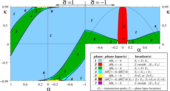
Figure 2: (color) The “phase diagram” of a two-level QD with $\tilde{a}_{L}=\tilde{a}_{R}=a$, $\tilde{b}_{L}=\tilde{\sigma}\tilde{b}_{R}=b$. The parameters are $U=0.1t$, $\tilde{E}_{1}^{(0)}=0$, $\tilde{E}_{2}^{(0)}=0.004t$, and $\sqrt{a^{2}+b^{2}}=0.125t$. The axes represent the 1-2 level asymmetry, $\alpha=(|a|-|b|)/\sqrt{a^{2}+b^{2}}$, and the dimensionless intra-dot hopping, $\kappa=w_{0}/[(\tilde{E}_{1}^{(0)}-\tilde{E}_{2}^{(0)})^{2}+w_{0}^{2}]^{1/2}$. Properties of different phases are summarized in the table. At $U\leq 0.04t$, the border of discontinuous-evolution region (bold line) does not meet the boundary between phases 1 and 2.

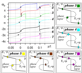
Figure 3: (color) Typical behavior of $\Theta_{tr}(\mu)$ in different phases (top left; plots shifted for convenience). Relative positions of transmission peaks (boxes; also in the main panel) and the $-\pi$-PLs (circles) in phases 3-7 are clarified by the schematic plots of $E_{1}-\mu$ around the multiple-solution region (absent for phases 1-2). Solid (dashed) lines correspond to stable (unstable) solutions. The abrupt “switching” of solutions (vertical solid line) may either renormalize the PL (when the $-\pi$-lapse lies in the unstable region) or result in a positive jump of $\Theta_{tr}$.

In Eq. (14), the second term on the r.h. s. corresponds to cutting the link between sites $j=-1/2$ and $j=1/2$ of the wire. The two resulting leads are coupled to the QD by $V_{T}$ [Eq. (2)]. Since for a wire of a finite length $2L$, $\xi$ is related to the shifts of (discrete) energy levels under the effect of $V$, it is easy Anderson to express $\xi$ in terms of $\Theta_{tr}$, viz.

$$\xi=-\Theta_{tr}/\pi+m(\epsilon)$$ (15)

(see Appendix A). The integer-valued function $m$ should be chosen to satisfy the requirementiml for $\xi(\epsilon)$ to vanish continuously with decreasing strength of the perturbation (e.g., $\lambda V$ with $\lambda\rightarrow 0$). We find that the value of $m$ changes by $+1$ at $\epsilon=E_{1,2}$ [eigenvalues of ${\cal H}^{MF}_{d}$, Eq.(5)], and by $-1$ at the transmission zero. For $\tilde{\sigma}=-1$ we obtain (in the units where $t=1$):

$$\langle\tilde{d}^{\dagger}_{1}\tilde{d}_{1}\rangle = \int_{-1}^{\mu}\sqrt{1-\epsilon^{2}}\,X(\epsilon)d\epsilon\times$$

$$\!\!\!\times\left[a^{2}b^{4}(1-\epsilon^{2})+a^{2}(\tilde{E}_{2}-\epsilon+b^{2}\epsilon)^{2}+\frac{b^{2}w^{2}}{4}\right]\,,$$

$$\langle\tilde{d}^{\dagger}_{2}\tilde{d}_{2}\rangle = \int_{-1}^{\mu}\sqrt{1-\epsilon^{2}}\,X(\epsilon)d\epsilon\times$$

$$\!\!\!\times\left[a^{4}b^{2}(1-\epsilon^{2})+b^{2}(\tilde{E}_{1}-\epsilon+a^{2}\epsilon)^{2}+\frac{a^{2}w^{2}}{4}\right]\,,$$

$$\langle\tilde{d}^{\dagger}_{1}\tilde{d}_{2}\rangle = \frac{w}{2}\int_{-1}^{\mu}\sqrt{1-\epsilon^{2}}\,X(\epsilon)d\epsilon\times$$

$$\!\!\!\times\left[a^{2}(\tilde{E}_{2}-\epsilon)+b^{2}(\tilde{E}_{1}-\epsilon)+2a^{2}b^{2}\epsilon\right]\,,$$

$$\frac{1}{\pi X(\epsilon)}=(1-\epsilon^{2})\left[a^{2}(\tilde{E}_{2}-\epsilon)+b^{2}(\tilde{E}_{1}-\epsilon)+2a^{2}b^{2}\epsilon\right]^{2}\!\!+$$

$$+\!\left[(\tilde{E}_{1}-\epsilon+a^{2}\epsilon)(\tilde{E}_{2}-\epsilon+b^{2}\epsilon)\!-\!(1-\epsilon^{2})a^{2}b^{2}\!-\frac{1}{4}w^{2}\right]^{2}\!\!.$$

Similar expressions are obtained also for the $\tilde{\sigma}=1$ case (see Appendix B).

We now solve equations (6–7) numerically (v), and substitute the resulting values of $\tilde{E}_{1,2}$ and $w$ into the expression for $\Theta_{tr}$ to get the transmission phase (vi).

The results are summarized in the phase diagram, Fig. 2. The left-hand part corresponds to $\tilde{\sigma}=1$, whereas the $\tilde{\sigma}=-1$ case (when the results do not depend on the sign of $w_{0}$) is shown on the right. The bold line marks the boundary between continuous (phases 1-2) and discontinuous (see below) regimes of dependence of the effective QD parameters on $\mu$. Within each regime, different phases are identified according to the magnitude and location of PL(s) with respect to the transmission peaks (Fig. 2, table). It should be noted that in the $\tilde{\sigma}=-1$ case the latter are given by $\mu_{1,2}=(\tilde{E}_{1}+\tilde{E}_{2})/2\mp\frac{1}{2}[(\tilde{E}_{1}-\tilde{E}_{2})^{2}+w^{2}+4a^{2}b^{2}/t^{2}]^{1/2}$, and are slightly shifted with respect to mean field dot levels, $E_{1,2}$. In the table, we denote transmission peaks by $E_{1,2}$ irrespective of the sign of $\tilde{\sigma}$ in order to keep the notation uniform. Typical dependence of $\Theta_{tr}$ on $\mu$ for each phase is shown in Fig. 3.

In the continuous-evolution part, phase 1 (phase 2), which occupies a large (small) area of the phase space, corresponds to the case when the phase lapse of $-\pi$, associated with the transmission zero, lies within (outside) the interval of values of $\mu$ between the two transmission peaks. It should be noted that the right-hand, $\tilde{\sigma}=-1$, side is expected to be representative of both opposite- and same-sign cases ($\sigma=\pm 1$), provided that the left-right asymmetry is sufficiently strong (large $w_{0}$). This is illustrated by the thin solid line, above (below) which coupling signs for the two bare dot levels $E_{1,2}^{(0)}$ become the same, $\sigma=1$ (opposite, $\sigma=-1$). Once the interaction effects are taken into account, one sees that phase 1 extends also far below this line, which is indicative of the effective change of the coupling sign [due in turn to the interaction-induced enhancement of $w$; at $w\gg\tilde{E}_{2}-\tilde{E}_{1}$, the coupling of the two mean-field dot levels, $(\tilde{d}_{1}\pm\tilde{d}_{2})/\sqrt{2}$, to the leads is same-sign].

The discontinuous behavior is associated with the presence of multiple solutions of the mean field equations (6–7) within a range of values of $\mu$, which is illustrated by a “fold” (bold solid and dashed lines) on the schematic $E_{1}(\mu)-\mu$ plots in Fig. 3. We find that if a system formally is allowed to follow such a multiple-valued solution from left to right, the value of $\Theta_{tr}$ increases, and also suffers a PL of $-\pi$ at some point (marked by a circle). In reality, thermodynamics dictates that the full thermodynamic potential $\Omega=\Omega_{MF}-U\langle\tilde{d}^{\dagger}_{1}\tilde{d}_{1}\rangle\langle\tilde{d}_{2}^{\dagger}\tilde{d}_{2}\rangle+U\langle\tilde{d}_{1}^{\dagger}\tilde{d}_{2}\rangle^{2}$ [cf. Eq. (11)] should be minimized to identify the stable solution, resulting in a “jump” (vertical line), which in turn is associated with a positive increase of $\Theta_{tr}$ by a fraction of $\pi$, giving rise to a second “PL” (phases 4,6), and with the population switchingSI ; Baltin of the dot levels. If the transmission zero lies in the thermodynamically unstable part of the solution (bold dashed line; phases 3,5,7), the PL of $-\pi$ should be added to this positive increase of $\Theta_{tr}$, giving rise to a single “renormalized” PL. Finally, one of the transmission peaks may be located within the unstable region (phases 5,6) with a result that the plot of $\Theta_{tr}(\mu)$ does not have a corresponding inflection point, which is replaced by a PL.

It follows that at least within the mean-field framework discontinuous population switching is always associated with the presence of multiple solutions and hence with “renormalized” PLs (or alternatively with additional “PLs” characterized by an increase of phase by a fraction of $\pi$). This conclusion is clearly at variance with the suggestion of Ref. SI, that the discontinuous switching between multiple solutions gives rise to the PLs of $\pi$ as observed experimentally. We note that while the behavior of transmission phase in this regime should be investigated beyond the mean field, the main point of our paper is that there is another mechanism which gives rise to a PL of $\pi$ without a discontinuous population switching (phase 1). Since this latter scenario does not involve instabilities of any kind, it can be expected to remain robust with respect to fluctuations (not included in the present treatment).

In summary, we have presented here a generic mechanism for the appearance of phase lapses between Coulomb blockade peaks. These PLs may be renormalized by a discontinuous ”population switching”. Experimentally it would be interesting to correlate the latter with the former by simultaneously measuring dot occupancy (employing a quantum point contact), and transmission phase. Theoretically, going beyond a mean field analysis is needed to determine the importance of quantum fluctuations.

The authors thank R. Berkovits, M. Heiblum, I. V. Lerner, V. Meden, and Y. Oreg for enlightening discussions. This work was supported by the ISF (grant No. 193/02-1 and the Centers of Excellence Program), by the EC RTN Spintronics, the BSF (grants # 2004162 and # 703296), and by the Israeli Ministry of Absorption. YG was also supported by an EPSRC fellowship.

Appendix A Spectral Shift Function, Transmission Phase, and Friedel Sum Rule

For the case at hand, the use of the standard formulaiml for the spectral shift function $\xi$,

$$\xi(\epsilon)=-\frac{1}{\pi}{\rm Arg}\,{\rm Det}\left\{\hat{1}-\frac{1}{\epsilon-{\rm i0}-{\cal H}_{w}-{\cal H}_{d}^{MF}}\hat{V}\right\}\,,$$ (19)

proves rather cumbersome. Instead, we will use the underlying notion of spectral shiftsiml in order to derive the generic relation (15) between $\xi$ and the transmission phase. This derivation also allows for an important insight concerning the Friedel sum rule.

We consider a system similar to that shown in Fig. 1, with the QD between the sites $-1/2$ and $1/2$ replaced by an arbitrary point scatterer. The latter is characterized by an $S$-matrix whose elements have a smooth dependence on the particle energyblackbox . While the boundary conditions cannot affect the value of $\xi$ in the limit when the length of the wire, $2L$, is large, the treatment is simpler when periodic boundary conditions are assumed. The spectrum of the wire in the absence of the scatterer, which we refer to as unperturbed, is then given by

$$\epsilon(k_{j})=-\cos k_{j}\,,\,\,\,\,k_{j}=\frac{\pi j}{L}\,,\,\,\,j=0,1,2,...,L$$ (20)

[cf. Eq. (12) where we assumed $t=1$]. The wave functions are proportional to $\exp{(\pm{\rm i}k_{j}x)}$ and, for $j\neq 0,L$, the corresponding energy levels are doubly degenerate. Since we are ultimately interested in the $L\rightarrow\infty$ limit, it is assumed that the inter-level spacing in the wire constitutes the smallest energy scale in the problem. The levels are shifted, and the degeneracy is lifted, in the presence of the scatterer, when the wave function is generally given by

$$\psi(x)=\left\{\begin{array}[]{ll}A_{1}{\rm e}^{{\rm i}kx}+B_{1}{\rm e}^{-{\rm i}kx},&x<0,\\ A_{2}{\rm e}^{{\rm i}kx}+B_{2}{\rm e}^{-{\rm i}kx},&x>0.\end{array}\right.$$ (21)

The linear relationship between coefficients on the right and on the left of the scatterer reads (assuming time-reversal symmetry)LL :

$$A_{2}=\alpha A_{1}+\beta B_{1}\,,\,\,\,B_{2}=\beta^{*}A_{1}+\alpha^{*}B_{1}$$ (22)

with $|\alpha|^{2}-|\beta|^{2}=1$. Relation of the quantities $\alpha$ and $\beta$ to the $S$-matrix is given by, e.g., setting $A_{1}=0$ (incoming particle from the right), hence (right-right) reflection amplitude, $r_{rr}=\beta/\alpha^{*}$ and transmission amplitude, $t_{tr}=1/\alpha^{*}$.

Now the periodic boundary conditions dictate that the allowed momentum values shift,

$$k_{j}\rightarrow k^{(1,2)}_{j}=k_{j}+\frac{\Delta^{(1,2)}_{j}\pi}{L},$$ (23)

Substituting Eqs. (21–23) into the condition $\psi(-2L+0)=\psi(+0)$, we find for $l=1,2$

$$A_{1}{\rm e}^{-2\pi{\rm i}\Delta^{(l)}} = A_{2}=\alpha A_{1}+\beta B_{1},$$

$$B_{1}{\rm e}^{2\pi{\rm i}\Delta^{(l)}} = B_{2}=\beta^{*}A_{1}+\alpha^{*}B_{1}.$$

This yields the equation for $\Delta_{j}^{(1,2)}$ (cf. Ref. Anderson, ):

$$\alpha{\rm e}^{4\pi{\rm i}\Delta^{(l)}}-2{\rm e}^{2\pi{\rm i}\Delta^{(l)}}+\alpha^{*}=0,$$ (24)

or equivalently

$$\left({\rm e}^{2\pi{\rm i}\Delta^{(l)}}-{\rm e}^{2\pi{\rm i}\Delta^{(1)}_{j}}\right)\left({\rm e}^{2\pi{\rm i}\Delta^{(l)}}-{\rm e}^{2\pi{\rm i}\Delta^{(2)}_{j}}\right)=$$

$$={\rm e}^{4\pi{\rm i}\Delta^{(l)}}-\frac{2}{\alpha}{\rm e}^{2\pi{\rm i}\Delta^{(l)}}+\frac{\alpha^{*}}{\alpha},$$

yielding

$${\rm e}^{2\pi{\rm i}(\Delta^{(1)}_{j}+\Delta^{(2)}_{j})}=\frac{\alpha^{*}}{\alpha}\,.$$ (25)

In the limit $L\rightarrow\infty$, the quantities $\Delta^{(1,2)}_{j}$ become functions of energy and, writing also $\alpha={\rm exp}({{\rm i}\Theta_{tr}})/|t_{tr}|$ with $\Theta_{tr}$ the transmission phase, we find

$$\Delta[\epsilon(k_{j})]\equiv\Delta^{(1)}_{j}+\Delta^{(2)}_{j}=-\frac{1}{\pi}\Theta_{tr}[\epsilon(k_{j})]+m[\epsilon(k_{j})]\,.$$ (26)

Let us now discuss the quantities appearing in Eq. (26). (i) $\Theta_{tr}$ is the transmission phase. In the presence of localized states within the scatterer (dot levels $E^{d}_{i}$), $\Theta_{tr}$ increases by $\pi$ as the energy of interest [$\epsilon(k_{j})$ in our notation, or more physically, the chemical potential] spans a resonance. (ii) $m(\epsilon)$ is an integer which we will now choose in such a way that $\Delta$ coincides with the Lifshits – Krein spectral shift function, $\xi(\epsilon)$ [see Eq. (13)]. $m(\epsilon)$ then changes by $+1$ with increasing energy at every $E^{d}_{i}$; in addition, it changes by $-1$ at the points where transmission vanishes (transmission PLs). We thus arrive at Eq. (15). (iii) $\Delta^{(1)}_{j}\pi/L$ and $\Delta^{(2)}_{j}\pi/L$ are the shifts in the allowed values of momentum [cf Eq. (23)].

There is no bound state corresponding to a PL, implying that $\xi(\epsilon)$ should be continuous at that point (transmission zero). The choice of $m(\epsilon)$ discussed above [along with Eq. (26)], ensures that $\Delta$ indeed may be synonymous with $\xi$ (see below).

In order to use the calculated value of spectral shift function for the total energy evaluation via the trace formula, Eq. (11), one needs to know the overall additive constant in $\xi(\epsilon)$. In the regime of interest to us, no bound state is formed below the band bottom (at $\epsilon<-1$). From the viewpoint of the lowest-energy electron states ($\epsilon\rightarrow-1+0$), the scatterer then acts as an impenetrable potential barrier (and not as a potential well), and the constant is fixed by a readily derivable condition, $\xi(\epsilon\rightarrow-1+0)=1/2$, valid for any barrier with no bound state formed below its bottom.

The quantity $\xi(\epsilon)$ remains a smooth function of energy $\epsilon$ away from band edges $\epsilon=\pm 1$ and the dot levels ${E}^{d}_{i}$. As mentioned in the text, the spectral shift function is related to the perturbation-induced change in the density of states. For the unperturbed system, the latter can be defined in the $L\rightarrow\infty$ limit only as

$$\nu_{0}[\epsilon(k_{j})]=\lim_{L\rightarrow\infty}\frac{2}{\epsilon(k_{j+1})-\epsilon(k_{j})}\propto L\,,$$ (27)

where the factor of $2$ reflects the double degeneracy of energy levels. In the presence of the scatterer we obtain, with the help of Eq. (23),

$$\nu[\epsilon(k_{j})]=$$

$$=\lim_{L\rightarrow\infty}\frac{2}{\left[\epsilon(k_{j+1})-\epsilon(k_{j})\right]\left\{1+\frac{1}{2}\xi[\epsilon(k_{j+1})]-\frac{1}{2}\xi[\epsilon(k_{j})]\right\}}$$

$$=\nu_{0}[\epsilon(k_{j})]+\delta\nu[\epsilon(k_{j})]\,,\,\,\,\,$$

where

$$\delta\nu(\epsilon)=-d\xi(\epsilon)/d\epsilon\,.$$ (28)

Here, we used the obvious fact that the centre of gravity of the two perturbed levels formed out of a doubly degenerate unperturbed level $\epsilon(k_{j})$ is given by $\epsilon(k_{j})+\frac{1}{2}[\epsilon(k_{j+1})-\epsilon(k_{j})]\Delta[\epsilon(k_{j})]$ (substituting $\Delta$ with $\xi$ for our choice of $m$). We note that, as expected on physical grounds, the quantity $\delta\nu$ is not extensive, i. e., it is not proportional to the length of the wire (in contrast to $\nu_{0}$). For the specified choice of $m(\epsilon)$ in Eq. (26), Eq. (28) yields also a delta-functional contribution to $\delta\nu$ of the form $-\sum_{i}\delta(\epsilon-{E}^{d}_{i})$. This corresponds to merging of the discrete dot levels into continuum and shows that $\delta\nu$ is the difference in the density of states between the wire with the scatterer and a disconnected system comprised of an unperturbed wire alongside an isolated scatterer.

Integrating Eq. (28), we get the expression for the total particle number,

$$N(\mu)=N^{(0)}_{wire}(\mu)+\sum_{i}\theta(\mu-{E}_{i}^{d})-\xi(\mu)\,,$$ (29)

where the first term on the r. h. s. is the band filling of an unperturbed wire. By re-writing this in terms of transmission phase $\Theta_{tr}(\epsilon)$ [cf. Eq. (26)], we get the Friedel sum rule in the form

$$N(\mu)=N^{(0)}_{wire}(\mu)+\Theta_{tr}(\mu)/\pi+\tilde{m}(\mu)$$ (30)

With increasing $\mu$, the integer $\tilde{m}$ changes by $+1$ at transmission zeroes, $\mu=Z_{i}$. We note that the sum of the two last terms on the r. h. s. of Eq. (30) remains continuous at $\mu=Z_{i}$, emphasizing that the Friedel sum rule does not account for the transmission phase lapses. This is because the underlying spectral characteristic, $\xi(\epsilon)$ [cf. Eq. (29)] remains smooth at $\mu=Z_{i}$ and in general does not depend on $|t_{tr}|$.

Appendix B Mean-Field Equations in the ${\mathbf{\tilde{\sigma}=1}}$ Case

In the case of same-sign symmetric coupling of the QD to the leads, $\tilde{\sigma}=1$, Eqs. (8–9) and (Transmission through Quantum Dots: Focus on Phase Lapses–Transmission through Quantum Dots: Focus on Phase Lapses) are replaced with

$$\sqrt{t^{2}-\epsilon^{2}}\,{\rm tan}\Theta_{tr}=\epsilon+\frac{b^{2}(\tilde{E}_{1}-\epsilon)+a^{2}(\tilde{E}_{2}-\epsilon)+abw}{(\tilde{E}_{1}-\epsilon)(\tilde{E}_{2}-\epsilon)-\frac{1}{4}w^{2}}\,,$$

$$Z=\frac{\tilde{E}_{2}a^{2}+\tilde{E}_{1}b^{2}+abw}{a^{2}+b^{2}}\,$$

and

$$\langle\tilde{d}^{\dagger}_{1}\tilde{d}_{1}\rangle = \int_{-1}^{\mu}\sqrt{1-\epsilon^{2}}\left[a(\tilde{E}_{2}-\epsilon)+\frac{1}{2}bw\right]^{2}Y(\epsilon)d\epsilon\,,$$

$$\langle\tilde{d}^{\dagger}_{1}\tilde{d}_{1}\rangle = \int_{-1}^{\mu}\sqrt{1-\epsilon^{2}}\left[b(\tilde{E}_{1}-\epsilon)+\frac{1}{2}aw\right]^{2}Y(\epsilon)d\epsilon\,,$$

$$\langle\tilde{d}^{\dagger}_{1}\tilde{d}_{2}\rangle = \int_{-1}^{\mu}\sqrt{1-\epsilon^{2}}\,Y(\epsilon)d\epsilon\times$$

$$\times\left[a(\tilde{E}_{2}-\epsilon)+\frac{1}{2}bw\right]\cdot\left[b(\tilde{E}_{1}-\epsilon)+\frac{1}{2}aw\right]\,,$$

respectively. Here,

$$\frac{1}{\pi Y(\epsilon)} = (1-\epsilon^{2})\left[(\tilde{E}_{1}-\epsilon)(\tilde{E}_{2}-\epsilon)-\frac{1}{4}w^{2}\right]^{2}+$$

$$+\left\{a^{2}(\tilde{E}_{2}-\epsilon)+b^{2}(\tilde{E}_{1}-\epsilon)+abw+\begin{array}[]{c}\\ \end{array}\right.$$

$$+\left.\epsilon\left[(\tilde{E}_{1}-\epsilon)(\tilde{E}_{2}-\epsilon)-\frac{1}{4}w^{2}\right]\right\}^{2}.$$