On a theoretical model for d-wave to mixed s- and d-wave transition in cuprate superconductors
Abstract
-
Department of Physics Technion-Israel Institute of Technology, Haifa 32000 Israel
-
Abstract. A model proposed by Iachello for superconductivity in cuprate materials is analyzed. The model consists of s and d pairs (approximated as bosons) in a two-dimensional Fermi system with a surface. The transition occurs between a phase in which the system is a condensate of one of the bosons, and a phase which is a mixture of two types of bosons. In the current work we have investigated the validity of the Bogoliubov approximation, and we used a reduced Hamiltonian to determine a phase diagram, the symmetry of the phases and the temperature dependence of the heat capacity.
-
Department of Physics Technion-Israel Institute of Technology, Haifa 32000 Israel
-
Abstract. A model proposed by Iachello for superconductivity in cuprate materials is analyzed. The model consists of s and d pairs (approximated as bosons) in a two-dimensional Fermi system with a surface. The transition occurs between a phase in which the system is a condensate of one of the bosons, and a phase which is a mixture of two types of bosons. In the current work we have investigated the validity of the Bogoliubov approximation, and we used a reduced Hamiltonian to determine a phase diagram, the symmetry of the phases and the temperature dependence of the heat capacity.
For more than a decade there has been a debate regarding the nature of the symmetry of the macroscopic wavefunction for the copper oxide superconductors. According to Müller bulk sensitive experiments support substantial s symmetry, while surface sensitive experiments yield d symmetry for the macroscopic wave function. Müller proposed [1] that a reconciliation of the conflicting experiments was possible if the superconducting wavefunction were a sum of two components, namely, one of s symmetry and one of d symmetry, and varied as a function of the distance from the surface.
Following that work by Müller, a theoretical framework for cuprate superconductors was proposed by Iachello [2], based on the analogy with atomic nuclei. In the present work we report our analysis of phase transitions based on Iachello’s model. Also we have investigated temperature dependence of the heat capacity. We propose a macroscopic wavefunction for realizing space dependence.
In Eq. ‣ On a theoretical model for d-wave to mixed s- and d-wave transition in cuprate superconductors we give Iachello’s Hamiltonian for spin fermions on a plane. This is a boson Hamiltonian [3] , which consists of three types of bosons , and .
Introducing the operators [2]
(2) the Hamiltonian can be rewritten as
Its algebraic structure is
This algebra contains a subalgebra formed from the generators , , and a Casimir operator defined as (note a factor of difference from Ref. [2])
Following Iachello this Hamiltonian can be split into an symmetric part, which will contain and terms, and a symmetric part generated by and respectively. When the Hamiltonian has symmetry the system is in phase , which corresponds to a mixture of s- and d- bosons. When the Hamiltonian has symmetry the system is in phase , which corresponds to either an s-boson condensate (phase or a d-boson condensate (phase [2].
As shown in Ref. [2] an analytical solution could be obtained either for phase or phase , but in intermediate situations one could only obtain an approximate or a numerical solution. Since we have three kinds of bosons in the model and a macroscopic number of particles, we may use the Bogoliubov approximation [4]. This approximation consists of replacing in the Hamiltonian ( ‣ On a theoretical model for d-wave to mixed s- and d-wave transition in cuprate superconductors) the operators which create and annihilate bosons in the condensed state by a c-number and neglecting all terms higher than degree two in operators which annihilate and create bosons in other states. After this replacement the Hamiltonian becomes the bilinear form
where , and is a chemical potential. The chemical potential is determined as usual from the condition on the mean total number of particles. is determined by variation. To diagonalize the bilinear form ( ‣ On a theoretical model for d-wave to mixed s- and d-wave transition in cuprate superconductors) we introduce the squeezing transformation
We compare the Bogoliubov approximation with the exact numerical solution in Fig 1.
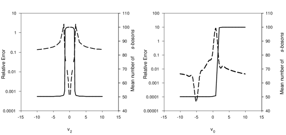
Figure 1: Relative error in the ground state energy (left y-axis, dashed line), calculated using the Bogoliubov approximation, and exact mean s-bosons population (right y-axis, solid line) versus parameters of the Hamiltonian. The fixed parameters are The right column of Fig 1 shows the occupancy of the s-bosons. We observe different regions of the parameter corresponding to different phases of the system. The left column shows that the Bogoliubov approximation gives remarkably good results either when the system is in phase or phase The failure of the Bogoliubov approximation in phase is expected since the s-level is not macroscopically occupied in that phase. (Another Bogoliubov approximation based on macroscopic occupancy of only d-bosons could be constructed for phase )
In order to investigate the transition between phase and phase the original Hamiltonian ( ‣ On a theoretical model for d-wave to mixed s- and d-wave transition in cuprate superconductors) can be reduced to the form
(5) by setting and This Hamiltonian contains the essential features required to describe the transition between the phases. The system is in phase for and it is in phase for In the first case the system reduces to a simple two level system of non-interacting bosons, and in the second case we have pure pairing interaction. In order to have a quantitative measure of s-wave and d-wave symmetry we define two fractional weight operators
and the fractional weight measures of a state
with the properties
where the subscripts and indicate respectively.
For pure s-wave symmetry and yield one and zero, respectively, and vice-versa for pure d-wave symmetry. For mixed symmetries, and vary between zero and one.
A phase diagram of the system described by the reduced Hamiltonian (5) may be obtained readily by calculating the s-wave or the d-wave symmetry measure in the exact ground state for different values of and
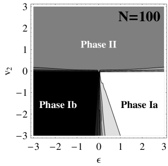
Figure 2: S-wave symmetry measure of the ground state calculated for various values of and Lighter tones denote higher values. As seen from Fig. 2 the system has three distinct phases. When the system is in phase the number of s- and d- bosons is definite; when it is in phase the number of s- and d-bosons is indefinite. The transition between the phases can be controlled by changing or
The strength of the scattering interaction could be controlled by the doping of the superconducting sample. It is known that doping affects electron-electron and electron-phonon scattering [5], therefore the desired scattering on the Fermi surface could be achieved by varying the doping of the sample (Meir Weger, private communication).
Having the exact numerical solution we can examine the thermodynamical properties of this model by calculating the free energy and the density matrix of the system at inverse temperature
We can then explore the behavior of the derivatives of the free energy with respect to the temperature. The first and the second derivatives of the free energy are shown to be continuous functions at the explored domain of parameters. However, there is a jump in the second derivative when the temperature scale is of the same order as the difference between the ground and first excited states (Fig 4).

Figure 3: The entropy (solid line) and the specific heat of the system (dashed line) as a function of the temperature. For the system is in phase 
Figure 4: Mean symmetry measures as functions of the temperature. The solid line denotes the s-wave symmetry measure and the dashed line denotes the d-wave symmetry measure. For the system is in phase This jump does not become a singularity point when the number of particles tends to infinity, since the width of the peak does not scale as , and therefore there is no second order phase transition at this point[6].
Although there is no second order phase transition, changing the temperature does produce a transition between phases having different symmetries. If the system is in phase at we can calculate the mean ensemble s-wave and d-wave symmetry measures as a function of the temperature
In Fig. 4 we present the temperature dependence of and We observe that both symmetry measures approach when the temperature is increased, which corresponds to phase of the system. If the system is initially in phase , it would remain in this phase for any temperature. It is tempting to propose the temperature as the control parameter for the transition, but some things should be kept in mind. First, the temperature scale of the transition may be higher than the critical temperature of the superconductor. This can only be known after the model is fit to experimental data and the values of the Hamiltonian parameters (5) are obtained. Second, if we would like the temperature to be the control parameter of the transition, there must be a temperature gradient within the copper-oxide plane of the superconductor, so that the bulk of the superconductor will have higher temperature than its surface. This is not likely to happen since the superconductor is in thermal equilibrium and the typical surface depth is of the order of only several atomic layers.
To sum up, in this work we have used a theoretical model proposed by Iachello [2] for a transition from d-wave to mixed d- and s-wave symmetry. A phase diagram of the model was obtained, which showed a distinct separation between the three phases. Doping of the superconducting sample and temperature were proposed as possible control parameters for the phases of the system.
Acknowledgements
We would like to thank Meir Weger for his considerable help. JLB thanks the Institute of Theoretical Physics of Technion for its support and hospitality. Also support from PSC-CUNY is acknowledged.
References
- [1] Müller K A 2002 Phil. Mag. Lett. 82 279; 1995 Nature 377 133; 2001 J. Supercond. 13 863
- [2] Iachello F 2002 Phil. Mag. Lett. 82 289, (This model was previously described by Bassichis and Foldy in 1964, in a different context: Bassichis W H and Foldy L L 1964 Phys. Rev. 133 A935; Bassichis W H and Disantnik Y 1966 Phys. Rev. 141 217)
- [3] Otsuka T, Arima A, and Iachello F 1978 Nucl. Phys. A 309 1
- [4] Bogoliubov N N 1947 J. Phys. (USSR) 11 23
- [5] Yeh N C et al 2001 Phys. Rev. Lett. 87 087003
- [6] Pathria R K 1996 Statistical Mechanics (Oxford: Butterworth-Heinemann)